
Abstract
We suggest new dual algorithms and iterative methods for solving monotone generalized variational inequalities. Instead of working on the primal space, this method performs a dual step on the dual space by using the dual gap function. Under the suitable conditions, we prove the convergence of the proposed algorithms and estimate their complexity to reach an  -solution. Some preliminary computational results are reported.
1. Introduction
Let  be a convex subset of the real Euclidean space
  ,
,  be a continuous mapping from
  into
into  , and
, and  be a lower semicontinuous convex function from
  into
into  . We say that a point
  is a solution of the following generalized variational inequality if it satisfies

where  denotes the standard dot product in
  .
.
Associated with the problem (GVI), the dual form of this is expressed as following which is to find  such that

In recent years, this generalized variational inequalities become an attractive field for many researchers and have many important applications in electricity markets, transportations, economics, and nonlinear analysis (see [1–9]).
It is well known that the interior quadratic and dual technique are powerfull tools for analyzing and solving the optimization problems (see [10–16]). Recently these techniques have been used to develop proximal iterative algorithm for variational inequalities (see [17–22]).
In addition Nesterov [23] introduced a dual extrapolation method for solving variational inequalities. Instead of working on the primal space, this method performs a dual step on the dual space.
In this paper we extend results in [23] to the generalized variational inequality problem (GVI) in the dual space. In the first approach, a gap function  is constructed such that
  , for all
  and
and  if and only if
  solves (GVI). Namely, we first develop a convergent algorithm for (GVI) with
  being monotone function satisfying a certain Lipschitz type condition on
  . Next, in order to avoid the Lipschitz condition we will show how to find a regularization parameter at every iteration
  such that the sequence
  converges to a solution of (GVI).
The remaining part of the paper is organized as follows. In Section 2, we present two convergent algorithms for monotone and generalized variational inequality problems with Lipschitzian condition and without Lipschitzian condition. Section 3 deals with some preliminary results of the proposed methods.
2. Preliminaries
First, let us recall the well-known concepts of monotonicity that will be used in the sequel (see [24]).
Definition 2.1.
Let  be a convex set in
  , and
, and  . The function
  is said to be
(i)pseudomonotone on  if
if

(ii)monotone on  if for each
  ,
,

(iii)strongly monotone on  with constant
  if for each
  ,
,

(iv)Lipschitz with constant  on
on  (shortly
  -Lipschitz), if

Note that when  is differentiable on some open set containing
  , then, since
  is lower semicontinuous proper convex, the generalized variational inequality (GVI) is equivalent to the following variational inequalities (see [25, 26]):
Find  such that

Throughout this paper, we assume that:
(A
1
) the interior set of  , int
, int  is nonempty,
(A
2
) the set  is bounded,
(A
3
) is upper semicontinuous on
  , and
, and  is proper, closed convex and subdifferentiable on
  ,
,
(A
4
) is monotone on
  .
.
In special case  , problem (GVI) can be written by the following.
Find  such that

It is well known that the problem (VI) can be formulated as finding the zero points of the operator  , where

The dual gap function of problem (GVI) is defined as follows:

The following lemma gives two basic properties of the dual gap function (2.7) whose proof can be found, for instance, in [6].
Lemma 2.2.
The function  is a gap function of (GVI), that is,
(i) for all
  ,
,
(ii) and
and  if and only if
  is a solution to (DGVI). Moreover, if
  is pseudomonotone then
  is a solution to (DGVI) if and only if it is a solution to (GVI).
The problem  may not be solvable and the dual gap function
  may not be well-defined. Instead of using gap function
  , we consider a truncated dual gap function
  . Suppose that
  fixed and
  . The truncated dual gap function is defined as follows:

For the following consideration, we define  as a closed ball in
  centered at
  and radius
  , and
, and  . The following lemma gives some properties for
  .
.
Lemma 2.3.
Under assumptions (A1)–(A4), the following properties hold.
(i)The function  is well-defined and convex on
  .
.
(ii)If a point  is a solution to (DGVI) then
  .
.
(iii)If there exists  such that
  and
and  , and
, and  is pseudomonotone, then
  is a solution to (DGVI) (and also (GVI)).
Proof.
-
(i)
Note that
 is upper semicontinuous on
  for
for  and
and  is bounded. Therefore, the supremum exists which means that
  is well-defined. Moreover, since
  is convex on
  and
and  is the supremum of a parametric family of convex functions (which depends on the parameter
  ), then
  is convex on
-
(ii)
By definition, it is easy to see that
 for all
  . Let
. Let  be a solution of (DGVI) and
  . Then we have
  (2.9)
(2.9)
 is upper semicontinuous on
  for
for  and
and  is bounded. Therefore, the supremum exists which means that
  is well-defined. Moreover, since
  is convex on
  and
and  is the supremum of a parametric family of convex functions (which depends on the parameter
  ), then
  is convex on
 for all
  . Let
. Let  be a solution of (DGVI) and
  . Then we have
In particular, we have

for all  . Thus

this implies  .
.
-
(iii)
For some
 ,
,  means that
  is a solution to (DGVI) restricted to
  . Since
  is pseudomonotone,
  is also a solution to (GVI) restricted to
  . Since
  , for any
  , we can choose
  sufficiently small such that
 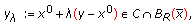 (2.12)
 ,
,  means that
  is a solution to (DGVI) restricted to
  . Since
  is pseudomonotone,
  is also a solution to (GVI) restricted to
  . Since
  , for any
  , we can choose
  sufficiently small such that

where (2.13) follows from the convexity of  . Since
  , dividing this inequality by
  , we obtain that
  is a solution to (GVI) on
  . Since
  is pseudomonotone,
  is also a solution to (DGVI).
Let  be a nonempty, closed convex set and
  . Let us denote
  the Euclidean distance from
  to
to  and
and  the point attained this distance, that is,

As usual,  is referred to the Euclidean projection onto the convex set
  . It is well-known that
  is a nonexpansive and co-coercive operator on
  (see [27, 28]).
The following lemma gives a tool for the next discussion.
Lemma 2.4.
For any  and for any
  , the function
  and the mapping
  defined by (2.14) satisfy


Proof.
Inequality (2.15) is obvious from the property of the projection  (see [27]). Now, we prove the inequality (2.16). For any
  , applying (2.15) we have

Using the definition of  and noting that
  and taking minimum with respect to
  in (2.18), then we have

which proves (2.16).
From the definition of  , we have

Since  , applying (2.15) with
  instead of
  and
and  for (2.20), we obtain the last inequality in Lemma 2.4.
For a given integer number  , we consider a finite sequence of arbitrary points
  , a finite sequence of arbitrary points
  and a finite positive sequence
  . Let us define

Then upper bound of the dual gap function  is estimated in the following lemma.
Lemma 2.5.
Suppose that Assumptions (A1)–(A4) are satisfied and

Then, for any  ,
,
(i) , for all
  ,
,  .
.
(ii) .
.
Proof.
-
(i)
We define
 as the Lagrange function of the maximizing problem
  . Using duality theory in convex optimization, then we have
 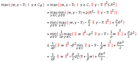 (2.23)
 as the Lagrange function of the maximizing problem
  . Using duality theory in convex optimization, then we have
(ii) From the monotonicity of  and (2.22), we have

Combining (2.24), Lemma 2.5(i) and

we get

3. Dual Algorithms
Now, we are going to build the dual interior proximal step for solving (GVI). The main idea is to construct a sequence  such that the sequence
  tends to 0 as
  . By virtue of Lemma 2.5, we can check whether
  is an
is an  -solution to (GVI) or not.
The dual interior proximal step  at the iteration
  is generated by using the following scheme:

where  and
and  are given parameters,
  is the solution to (2.22).
The following lemma shows an important property of the sequence  .
.
Lemma 3.1.
The sequence  generated by scheme (3.1) satisfies

where  ,
,  and
and  . As a consequence, we have

Proof.
We replace  by
by  and
and  by
by  into (2.16) to obtain

Using the inequality (3.4) with  ,
,  ,
,  and noting that
  , we get

This implies that

From the subdifferentiability of the convex function  to scheme (3.1), using the first-order necessary optimality condition, we have

for all  . This inequality implies that

where  .
.
We apply inequality (3.4) with  ,
,  and
and  and using (3.8) to obtain

Combine this inequality and (3.6), we get

On the other hand, if we denote  , then it follows that

Combine (3.10) and (3.11), we get

which proves (3.2).
On the other hand, from (3.9) we have

Then the inequality (3.3) is deduced from this inequality and (3.6).
The dual algorithm is an iterative method which generates a sequence  based on scheme (3.1). The algorithm is presented in detail as follows:
Algorithm 3.2.
One has the following.
Initialization:
Given a tolerance  , fix an arbitrary point
  and choose
  ,
,  . Take
  and
and  .
.
Iterations:
For each  , execute four steps below.
Step 1.
Compute a projection point  by taking

Step 2.
Solve the strongly convex programming problem

to get the unique solution  .
.
Step 3.
Find  such that

Set  .
.
Step 4.
Compute

If  , where
  is a given tolerance, then stop.
Otherwise, increase  by 1 and go back to Step 1.
Output:
Compute the final output  as:
as:

Now, we prove the convergence of Algorithm 3.2 and estimate its complexity.
Theorem 3.3.
Suppose that assumptions (A1)–(A3) are satisfied and  is
is  -Lipschitz continuous on
  . Then, one has

where  is the final output defined by the sequence
  in Algorithm 3.2. As a consequence, the sequence
  converges to 0 and the number of iterations to reach an
  -solution is
  , where
  denotes the largest integer such that
  .
.
Proof.
From  , where
  and
and  , we get

Substituting (3.20) into (3.2), we obtain

Using this inequality with  for all
  and
and  , we obtain

If we choose  for all
  in (2.21), then we have

Hence, from Lemma 2.5(ii), we have

Using inequality (3.22) and  , it implies that

Note that  . It follows from the inequalities (3.24) and (3.25) that

which implies that  . The termination criterion at Step 4,
  , using inequality (2.26) we obtain
  and the number of iterations to reach an
  -solution is
  .
.
If there is no the guarantee for the Lipschitz condition, but the sequences  and
and  are uniformly bounded, we suppose that

then the algorithm can be modified to ensure that it still converges. The variant of Algorithm 3.2 is presented as Algorithm 3.4 below.
Algorithm 3.4.
One has the following.
Initialization:
Fix an arbitrary point  and set
  . Take
  and
and  . Choose
  for all
  .
.
Iterations:
For each  execute the following steps.
Step 1.
Compute the projection point  by taking

Step 2.
Solve the strong convex programming problem

to get the unique solution  .
.
Step 3.
Find  such that

Set  .
.
Step 4.
Compute

If  , where
  is a given tolerance, then stop.
Otherwise, increase  by 1, update
  and go back to Step 1.
Output:
Compute the final output  as
as

The next theorem shows the convergence of Algorithm 3.4.
Theorem 3.5.
Let assumptions (A1)–(A3) be satisfied and the sequence  be generated by Algorithm 3.4. Suppose that the sequences
  and
and  are uniformly bounded by (3.27). Then, we have

As a consequence, the sequence  converges to 0 and the number of iterations to reach an
  -solution is
  .
.
Proof.
If we choose  for all
  in (2.21), then we have
  . Since
  , it follows from Step 3 of Algorithm 3.4 that

From (3.34) and Lemma 2.5(ii), for all  we have

We define  . Then, we have

We consider, for all 

Then derivative of  is given by

Thus  is nonincreasing. Combining this with (3.36) and
  , we have

From Lemma 3.1,  and
and  , we have

Combining (3.39) and this inequality, we have

By induction on  , it follows from (3.41) and
  that
that

From (3.35) and (3.42), we obtain

which implies that  . The remainder of the theorem is trivially follows from (3.33).
4. Illustrative Example and Numerical Results
In this section, we illustrate the proposed algorithms on a class of generalized variational inequalities (GVI), where  is a polyhedral convex set given by

where  ,
,  . The cost function
  is defined by

where  ,
,  is a symmetric positive semidefinite matrix and
  . The function
  is defined by

Then  is subdifferentiable, but it is not differentiable on
  .
.
For this class of problem (GVI) we have the following results.
Lemma 4.1.
Let  . Then
(i)if  is
is  -strongly monotone on
  , then
  is monotone on
  whenever
  .
.
(ii)if  is
is  -strongly monotone on
  , then
  is
is  -strongly monotone on
  whenever
  .
.
(iii)if  is
is  -Lipschitz on
  , then
  is
is  -Lipschitz on
  .
.
Proof.
Since  is
is  -strongly monotone on
  , that is

we have

Then (i) and (ii) easily follow.
Using the Lipschitz condition, it is not difficult to obtain (iii).
To illustrate our algorithms, we consider the following data.

with  ,
,  ,
,  . From Lemma 4.1, we have
  is monotone on
  . The subproblems in Algorithm 3.2 can be solved efficiently, for example, by using MATLAB Optimization Toolbox R2008a. We obtain the approximate solution

Now we use Algorithm 3.4 on the same variational inequalities except that

where the  components of the
  are defined by:
  , with
  randomly chosen in
  and the
  components of
  are randomly chosen in
  . The function
  is given by Bnouhachem [19]. Under these assumptions, it can be proved that
  is continuous and monotone on
  .
.
With  and the tolerance
  , we obtained the computational results (see, the Table 1).
 .
.References
Anh PN, Muu LD, Strodiot J-J: Generalized projection method for non-Lipschitz multivalued monotone variational inequalities. Acta Mathematica Vietnamica 2009, 34(1):67–79.
Anh PN, Muu LD, Nguyen VH, Strodiot JJ: Using the Banach contraction principle to implement the proximal point method for multivalued monotone variational inequalities. Journal of Optimization Theory and Applications 2005, 124(2):285–306. 10.1007/s10957-004-0926-0
Bello Cruz JY, Iusem AN: Convergence of direct methods for paramontone variational inequalities. Computational Optimization and Applications 2010, 46(2):247–263. 10.1007/s10589-009-9246-5
Facchinei F, Pang JS: Finite-Dimensional Variational Inequalities and Complementary Problems. Springer, New York, NY, USA; 2003.
Fukushima M: Equivalent differentiable optimization problems and descent methods for asymmetric variational inequality problems. Mathematical Programming 1992, 53(1):99–110. 10.1007/BF01585696
Konnov IV: Combined Relaxation Methods for Variational Inequalities. Springer, Berlin, Germany; 2000.
Mashreghi J, Nasri M: Forcing strong convergence of Korpelevich's method in Banach spaces with its applications in game theory. Nonlinear Analysis: Theory, Methods & Applications 2010, 72(3–4):2086–2099. 10.1016/j.na.2009.10.009
Noor MA: Iterative schemes for quasimonotone mixed variational inequalities. Optimization 2001, 50(1–2):29–44. 10.1080/02331930108844552
Zhu DL, Marcotte P: Co-coercivity and its role in the convergence of iterative schemes for solving variational inequalities. SIAM Journal on Optimization 1996, 6(3):714–726. 10.1137/S1052623494250415
Daniele P, Giannessi F, Maugeri A: Equilibrium Problems and Variational Models, Nonconvex Optimization and Its Applications. Volume 68. Kluwer Academic Publishers, Norwell, Mass, USA; 2003:xiv+445.
Fang SC, Peterson EL: Generalized variational inequalities. Journal of Optimization Theory and Applications 1982, 38(3):363–383. 10.1007/BF00935344
Goh CJ, Yang XQ: Duality in Optimization and Variational Inequalities, Optimization Theory and Applications. Volume 2. Taylor & Francis, London, UK; 2002:xvi+313.
Iusem AN, Nasri M: Inexact proximal point methods for equilibrium problems in Banach spaces. Numerical Functional Analysis and Optimization 2007, 28(11–12):1279–1308. 10.1080/01630560701766668
Kim JK, Kim KS: New systems of generalized mixed variational inequalities with nonlinear mappings in Hilbert spaces. Journal of Computational Analysis and Applications 2010, 12(3):601–612.
Kim JK, Kim KS: A new system of generalized nonlinear mixed quasivariational inequalities and iterative algorithms in Hilbert spaces. Journal of the Korean Mathematical Society 2007, 44(4):823–834. 10.4134/JKMS.2007.44.4.823
Waltz RA, Morales JL, Nocedal J, Orban D: An interior algorithm for nonlinear optimization that combines line search and trust region steps. Mathematical Programming 2006, 107(3):391–408. 10.1007/s10107-004-0560-5
Anh PN: An interior proximal method for solving monotone generalized variational inequalities. East-West Journal of Mathematics 2008, 10(1):81–100.
Auslender A, Teboulle M: Interior projection-like methods for monotone variational inequalities. Mathematical Programming 2005, 104(1):39–68. 10.1007/s10107-004-0568-x
Bnouhachem A: An LQP method for pseudomonotone variational inequalities. Journal of Global Optimization 2006, 36(3):351–363. 10.1007/s10898-006-9013-4
Iusem AN, Nasri M: Augmented Lagrangian methods for variational inequality problems. RAIRO Operations Research 2010, 44(1):5–25. 10.1051/ro/2010006
Kim JK, Cho SY, Qin X: Hybrid projection algorithms for generalized equilibrium problems and strictly pseudocontractive mappings. Journal of Inequalities and Applications 2010, 2010:-17.
Kim JK, Buong N: Regularization inertial proximal point algorithm for monotone hemicontinuous mapping and inverse strongly monotone mappings in Hilbert spaces. Journal of Inequalities and Applications 2010, 2010:-10.
Nesterov Y: Dual extrapolation and its applications to solving variational inequalities and related problems. Mathematical Programming 2007, 109(2–3):319–344. 10.1007/s10107-006-0034-z
Aubin J-P, Ekeland I: Applied Nonlinear Analysis, Pure and Applied Mathematics. John Wiley & Sons, New York, NY, USA; 1984:xi+518.
Anh PN, Muu LD: Coupling the Banach contraction mapping principle and the proximal point algorithm for solving monotone variational inequalities. Acta Mathematica Vietnamica 2004, 29(2):119–133.
Cohen G: Auxiliary problem principle extended to variational inequalities. Journal of Optimization Theory and Applications 1988, 59(2):325–333.
Mangasarian OL, Solodov MV: A linearly convergent derivative-free descent method for strongly monotone complementarity problems. Computational Optimization and Applications 1999, 14(1):5–16. 10.1023/A:1008752626695
Rockafellar RT: Monotone operators and the proximal point algorithm. SIAM Journal on Control and Optimization 1976, 14(5):877–898. 10.1137/0314056
Acknowledgments
The authors would like to thank the referees for their useful comments, remarks and suggestions. This work was completed while the first author was staying at Kyungnam University for the NRF Postdoctoral Fellowship for Foreign Researchers. And the second author was supported by Kyungnam University Research Fund, 2010.
Author information
Authors and Affiliations
Corresponding author
Rights and permissions
Open Access This article is distributed under the terms of the Creative Commons Attribution 2.0 International License (https://creativecommons.org/licenses/by/2.0), which permits unrestricted use, distribution, and reproduction in any medium, provided the original work is properly cited.
About this article
Cite this article
Anh, P., Kim, J. A New Method for Solving Monotone Generalized Variational Inequalities. J Inequal Appl 2010, 657192 (2010). https://doi.org/10.1155/2010/657192
Received:
Revised:
Accepted:
Published:
DOI: https://doi.org/10.1155/2010/657192