Feasible computation based on quantum logic

Abstract

The objective of this paper is to propose a feasible computational framework based on quantum logic. The usual quantum logic-based computational processes easily get stuck. The difficulty with the computation is ascribed to the difference in the inference rules for quantum and classical negations. It is shown that the new inference rule for negation which is akin to the classical one is partially applicable even to the quantum case. The resulting framework makes it possible to go beyond what the usual quantum logic-based computation could do.

1 Background

The objective of this paper is to propose a feasible computational framework based on quantum logic. The framework is formulated as a logic programming style, where the computation is expressed in Gentzen’s sequent calculus. In this section, we will briefly review these basic notions. For the general background of quantum computation, the reader may consult the thorough survey [8].

1.1 Quantum and classical logics

By the term quantum logic, we refer to a formal system modeled by the class of ortholattices¹ [5, 7]. Several studies have been conducted so far to investigate mathematical theories of computation based on quantum logic [12,13,14,15,16]. Considering the structure of ortholattice allows us to exploit the power of quantum logic, which has been investigated for over 80 years.

The most salient feature that differentiates quantum logic from classical one is its lack of distributivity of conjunction ($\wedge$) over disjunction ($\vee$). From the proof-theoretical point of view, this leads to a negative consequence that quantum logic does not admit any satisfactory implication operator ($\rightarrow$) [9]. Due to these defects, computational processes based on quantum logic easily get stuck.

The discontinuation between quantum and classical logics provokes a serious problem when we adopt the idea that the former governs the microscopic world and the latter governs the macroscopic world. Quantum logic differs qualitatively from classical logic in the sense that it violates, for example, the distributivity rule that holds in classical logic. Unlike physics where classical mechanics emerges as the continuous limit of quantum mechanics, logic has not yet been able to unify quantum and classical formulations that seem quite disparate on the surface.

Our strategy is to ascribe the difference between quantum and classical logics to that of the inference rules for negation. The negation rule of quantum logic is of a restricted form compared to that of classical logic. This simply means that quantum logic by itself fails to prove many classically valid theorems. A key point to note here is, however, that the classical negation rule still works in limited situations where the occurring propositions physically commute. Using this fact, we can formalize a feasible inference system even in quantum logic. We implement this computation technique in a logic programming framework.

1.2 Logic programming

Logic programming is a programming paradigm in which a logical inference process is seen as an execution of a program. A program is given as a set of rules of the form $a \rightarrow b$ where $a$ and $b$ are logical formulas. Positive facts (e.g. $\rightarrow b$; a rule with no premises) and negative facts (e.g. $a \rightarrow$; a rule with no conclusion) are also regarded as special kinds of rules.

Now we give a brief explanation of how the standard logic program operates. A program is driven by a negative fact, which is also referred to as a goal, say $c \rightarrow$, where c is a logical formula. Then by modus ponens, a new goal $a\theta \rightarrow$ (resp. $\lnot b\theta \rightarrow$) is obtained under the condition that a rule $a \rightarrow b$ belongs to the program and a matching $b\theta \equiv c\theta$ (resp. $\lnot a\theta \equiv c \theta$) of formulas is found for some substitution $\theta$ of variables. That is, an application of modus ponens can be considered as a goal rewriting process.

$$\begin{aligned}&\frac{a\theta \rightarrow b\theta \qquad c\theta \rightarrow }{ a\theta \rightarrow } \quad \quad \quad \quad \quad (b\theta \equiv c\theta ) \\&\frac{ a\theta \rightarrow b\theta \qquad c\theta \rightarrow }{ \lnot b\theta \rightarrow }\quad \quad \quad \quad \quad (\lnot a\theta \equiv c\theta ) \end{aligned}$$

Note that $a\theta \rightarrow b\theta$ is logically equivalent to $\lnot b\theta \rightarrow \lnot a \theta$. The matching operation of formulas is called unification, and the goal rewriting process that makes use of unification and modus ponens is called backchaining. This procedure is iterated until the goal is eventually reduced to one with no premises ($\rightarrow$;the empty goal, which means a contradiction). The celebrated Prolog treats only formulas of the restricted form called Horn clauses, which contain at most one positive literal. For formulas of the unrestricted form, which will be employed in this paper, consult the work of Bowen [3].

1.3 Sequent calculus

In the subsequent sections, we develop a method to carry out quantum-logical calculation by employing unification and backchaining mechanisms as logical inference rules. The particular form of representation we use is Gentzen-style sequent calculus. A sequent $\varGamma \vdash \varDelta$ is an expression that denotes a deducibility relation between sets $\varGamma$ and $\varDelta$ of formulas: assuming (all formulas in) $\varGamma$ holds we can conclude that (some formulas in) $\varDelta$ holds. Then a formal proof is formulated as a sequent-rewriting procedure. Studies on the sequent-style formulation of logic programming are found in the literature [4, 6, 10]. A sequent calculus for quantum logic has been introduced by Nishimura [11].

Compared to classical sequent calculus, the most distinctive feature of Nishimura’s quantum version consists in the inference rules for negation. The distinction is essentially ascribed to the presence or absence of distributivity of conjunction over disjunction. When interpreted physically, the distributivity of operations corresponds to the commutativity of observables. Section 4 gives details of this.

2 Representation of physical propositions

This section defines the symbols and terminology that we use to describe propositions in quantum logic, illustrating their intuitive meanings.

We use the following symbols.

• i. Atomic formulas

  • $p, q, r, \dots$, or $p_1, p_2, p_3, \dots , q_1, q_2, q_3, \dots$.

• ii. Logical connectives

  • $\wedge$ (conjunction)

  • $\vee$ (disjunction)

  • $\lnot$ (negation)

  • $\forall$ (universal quantification)

  • $\exists$ (existential quantification)

Atomic formulas refer to indistinguishable units of assertions, which can be combined to form more complex formulas with the help of logical connectives. The letters $a, b, c,\dots$, or $a_1, a_2, a_3,\dots$ are used as metavariables for formulas. An atomic formula $p$ that contains variables $x_1, x_2, \dots , x_n$ is also called a propositional function and may be denoted by $p(x_1, x_2, \dots , x_n)$. For a first-order domain $D$ and terms $t_1, t_2, \dots \, t_n$ in $D$, the value $p(t_1, t_2, \dots , t_n)$ of $p$ at $t_1, t_2, \dots \, t_n$ is a proposition. Intuitively, for instance, if we set

• $p(x)$: ‘the spin of the spin-half particle $P$ along the $Z$-axis is $x$.’

• $D$ : $\{\text {`up'}, \text {`down'}\}$

then we have

• $p(\text {`up'})$: ‘the spin of the spin-half particle $P$ along the $Z$-axis is up.’

In the same situation, we also have

• $\exists x \in D.p(x)$: ‘the spin of the spin-half particle $P$ along the $Z$-axis is either up or down.’ (quantum superposition)

The use of first-order variables and quantifiers to represent quantum superposition was inspired by the work of Battilotti² [1, 2].

For an atomic formula $p$, $p$ itself is said to be a positive literal, while $\lnot p$ a negative literal. A clause is a disjunction of positive or negative literals in which all variables are universally quantified. Due to the commutativity and associativity of the disjunction, we may assume without loss of generality that a clause is of the form where negative literals precede positive ones:

$$\forall x_1\forall x_2 \dots \forall x_l.(\lnot p_1 \vee \lnot p_2 \vee \dots \vee \lnot p_m \vee q_1 \vee q_2 \vee \dots \vee q_n)$$

(including the cases where $l = 0$). In classical logic, it is equivalent to the formula of the implication form

$$\forall x_1 \forall x_2 \dots \forall x_l.((p_1 \wedge \dots \wedge p_m) \rightarrow (q_1 \vee \dots \vee q_n))\mathrm {.}$$

Unfortunately, however, quantum logic does not admit the usual implication operation ($\rightarrow$) [9]. For this reason, we avoid using the implication operation ($\rightarrow$) in representing clauses. The negated form of a clause is called a goal³ which is written as

$$\lnot \forall x_1 \forall x_2 \dots \forall x_l.(\lnot p_1 \vee \lnot p_2 \vee \dots \vee \lnot p_m \vee q_1 \vee q_2 \vee \dots \vee q_n)\mathrm {.}$$

By applying De Morgan’s law, which will be described below, we may rewrite this as

$$\exists x_1 \exists x_2 \dots \exists x_l.(p_1 \wedge p_2 \wedge \dots \wedge p_m \wedge \lnot q_1 \wedge \lnot q_2 \wedge \dots \wedge \lnot q_n)\mathrm {.}$$

Finally, a finite set of clauses is called a logic program.

3 Inference rules for quantum sequents

Let $\varGamma$ and $\varDelta$ be finite (possibly empty) sets of formulas and $a_1, a_2, \dots a_n$ formulas. In sequents, expressions such as $\varGamma , a_1, a_n, \dots , a_n$ or $a_1, a_2, \dots , a_n, \varGamma$ are used as shorthand for $\varGamma \cup \{a_1, a_2, \dots , a_n\}$. The following inference rules for quantum sequents are originally due to Nishimura [11].

• i. Structure

  $$\frac{ \varGamma ' \vdash \varDelta '}{\varGamma \vdash \varDelta }$$

  where $\varGamma ' \subseteq \varGamma$ and $\varDelta ' \subseteq \varDelta$. Uses of the structural rule are sometimes not explicitly mentioned.

• ii. Cut

  $$\frac{ \varGamma \vdash \varDelta , a \qquad \varGamma , a \vdash \varDelta }{ \varGamma \vdash \varDelta }$$

• iii. $\wedge$ -left

  $$\frac{ \varGamma , a, b \vdash \varDelta }{ \varGamma , a \wedge b \vdash \varDelta }$$

• iv. $\wedge$ -right

  $$\frac{ \varGamma \vdash \varDelta , a \qquad \varGamma \vdash \varDelta , b }{ \varGamma \vdash \varDelta , a \wedge b }$$

• v. $\lnot$ -left

  $$\frac{ \varGamma \vdash \varDelta , a }{ \varGamma , \lnot a \vdash \varDelta }$$

• vi. $\lnot$ -right

  $$\frac{ a \vdash \varDelta }{ \lnot \varDelta \vdash \lnot a }$$

  where $\lnot \varDelta$ is the set of all negated formulas of $\varDelta$.

• vii. $\lnot \lnot$ -left

  $$\frac{ \varGamma , a \vdash \varDelta }{ \varGamma , \lnot \lnot a \vdash \varDelta }$$

• viii. $\lnot \lnot$ -right

  $$\frac{ \varGamma \vdash \varDelta , a }{ \varGamma \vdash \varDelta , \lnot \lnot a }$$

  The rules vii and viii are used to eliminate double-negations that appear in the proof. The application of these rules may not be explicitly written.

• ix. $\forall$ -left

  $$\frac{ \varGamma , a[\,?\,] \vdash \varDelta }{ \varGamma , \forall x\in D.a[\,x\,] \vdash \varDelta }$$

  where $a[\,x\,]$ is a formula that may contain x, and $a[\,?\,]$ is the same formula as $a[\,x\,]$ except that x is substituted with any term ? in D.

Remark 1

The formulas listed on the left side of the $\vdash$ sign constitute the set of all premises, and those on the right side constitute the set of possible conclusions. That is, $\varGamma \vdash \varDelta$ represents the proof-theoretic assertion that

if all formulas in $\varGamma$ hold (in quantum logic), then some formulas in $\varDelta$ hold (in quantum logic). (*)

The point to notice here is that the assertion (*) itself is made in the metalanguage, which is, of course, governed by classical logic. This means that the terms all and some in (*) should be interpreted classically. Hence (*) differs from the following assertion:

if the conjunction of all formulas in $\varGamma$ hold (in quantum logic), then the disjunction of all formulas in $\varDelta$ hold (in quantum logic). (**)

For comparison, consider the case of classical sequent calculus where $\varGamma \vdash \varDelta$ represents the proof-theoretic assertion that

if all formulas in $\varGamma$ hold (in classical logic), then some formulas in $\varDelta$ hold (in classical logic). (*CL)

In this case, both the object and the metalogic are classical logic. Hence (*CL) coincides with the following assertion:

if the conjunction of all formulas in $\varGamma$ hold (in classical logic), then the disjunction of all formulas in $\varDelta$ hold (in classical logic). (**CL)

What is the implication of these observations? In classical sequent calculus, a comma between formulas on the left side of the $\vdash$ sign is interchangeable with a conjunction sign ($\wedge$), and one on the right side a disjunction sign ($\vee$). While the former is still true in the quantum case⁴, the latter is not: a comma between formulas on the right side of the $\vdash$ sign is not interchangeable with a disjunction sign. With this fact in mind, we introduce the operation $\vee$ not via the inference rules of sequents, but via the following De Morgan’s law:

$$a \vee b \equiv \lnot (\lnot a\wedge \lnot b)\mathrm {.}$$

Uses of De Morgan’s law are not explicitly mentioned hereafter. Likewise, we introduce the quantifier $\exists$ via

$$\exists x \in D. a[x] \equiv \lnot \forall x \in D.\lnot a[x]\text {.}$$

Then the following inference rule may be derived:

$$\frac{ \varGamma \vdash a[\,?\,] }{ \varGamma \vdash \exists x\in D.a[\,x\,] }\quad \quad \quad \quad \quad \quad \quad (\exists \textsc {-right})$$

When each side of the $\vdash$ sign contains only a single formula, the deducibility relation $\vdash$ can be seen as a partial order relation $\le$. With this ordering, the set of all formulas forms an ortholattice. Sometimes the following additional axiom is adopted for this lattice to be orthomodular [5]:

$$a \wedge (\lnot a \vee (a \wedge b)) \vdash b\mathrm {.}$$

Remark 2

One apparent difference between classical and quantum sequent calculus consists in $\lnot$ -right rule (vi). The classical $\lnot$ -right rule is stated as follows:

$$\frac{ \varGamma , a \vdash \varDelta }{ \varGamma \vdash \lnot a, \varDelta }\quad \quad \quad \quad \quad \quad \quad (\lnot \textsc {-right (CL)})$$

Assuming $\lnot$ -right (CL), we obtain $\lnot$ -right of the quantum version as follows:

However, the converse is not provable. Hence, it may be said that $\lnot$ -right is weaker than $\lnot$ -right (CL). This distinction stems from the noncommutativity of observables. We examine this point in more details in the next section.

4 Relations between distributivity, commutativity, and $\lnot$-rule

The distinction between quantum and classical logics has commonly been ascribed to the presence or absence of the distributivity of $\wedge$ over $\vee$, or, that of the commutativity of observables in the corresponding physical theory. In the previous section, we observed that the crux of the distinction between both logics lies in the $\lnot$ -right rule of the corresponding sequent calculus. In this section, we examine the relations between these three properties: distributivity, commutativity, and $\lnot$ -right rule.

4.1 Distributivity

Let $a, b$ and $c$ be formulas. The following sequent represents the distributivity of $a$ over $b$ and $c$, and is written as $\mathrm {D}(a, b, c)$ for brevity:

$$a \wedge (b \vee c) \vdash (a \wedge b) \vee (a \wedge c)\mathrm {.}$$

Note that even in quantum sequent calculus, the reverse direction of the distributivity always holds. In fact, the following diagram depicts the proof of $(a \wedge b) \vee (a \wedge c) \vdash a \wedge (b \vee c)$.

4.2 Commutativity

The sequent $a \vdash (a \wedge b) \vee (a \wedge \lnot b)$ represents the commutativity of $a$ and $b$, and is written as $\mathrm {C}(a, b)$ for brevity. In fact, the following proposition holds.

Proposition 1

The sequents $\mathrm {C}(a, b)$ and $\mathrm {C}(b, a)$ are both valid in a Hilbert space model in which the subspaces $a$ and $b$ commute.

Proof

Note that two subspaces commute if and only if their projection operators commute. By abuse of notation, we use the same symbols $a, b$ and $c$ for their corresponding subspaces of some Hilbert space ${\mathbb {H}}$, with the superscript $\bot$ denoting the orthocomplement in ${\mathbb {H}}$. We have $ab^{\bot } = a(I-b) = a - ab$ where $I$ is the identity operator. Then we have $a = ab + ab^{\bot }$. Thus $a \le ab + ab^{\bot }$ which means that the sequent $a \vdash (a\wedge b) \vee (a\wedge \lnot b)$ is valid in this model. By the same token, it can be shown that $b \vdash (b\wedge a) \vee (b\wedge \lnot a)$ is valid. $\square$

Conversely, the following proposition also holds.

Proposition 2

In a Hilbert space model in which the sequents $\mathrm {C}(a, b)$ and $\mathrm {C}(b, a)$ are both valid, the subspaces $a$ and $b$ commute.

Proof

Suppose that $a \vdash (a\wedge b) \vee (a\wedge \lnot b)$ and $b \vdash (b\wedge a) \vee (b\wedge \lnot a)$ are both valid. This means that the inequalities $a \le ab + ab^{\bot }$ and $b \le ba + ba^{\bot }$ both hold in this model. Since the reverse inequalities $ab + ab^{\bot } \le a$ and $ba + ba^{\bot } \le b$ both hold in any (complemented) lattice, it follows that the equalities $a = ab + ab^{\bot }$ and $b = ba + ba^{\bot }$ both hold (*). For notational simplicity, let $a' = ab^{\bot }, b' = ba^{\bot }$, and $c = ab$. Then we have $a'c = 0, b'c = 0$ and $a'b' = 0$ which mean that $a' , b'$ and $c$ are mutually orthogonal. Since it follows from (*) that $a = c + a'$ and $b = c + b'$, we have $ab = (a' + c)(b' + c) = a'b' + a'c + cb' + cc = c$ and $ba = (b' + c)(a' + c) = b'a' + b'c + ca' + cc = c$ from which we conclude that $ab = ba$. $\square$

In quantum theory, if $a$ and $b$ commute, then of course $b$ and $a$ commute. Furthermore, the theory requires that $a$ and $\lnot b$, $\lnot a$ and $b$, and $\lnot a$ and $\lnot b$ also commute. Therefore, it is reasonable to require that in a Hilbert space model in which $a$ and $b$ commute, the following four axioms be introduced all together:

• $\mathrm {C}(a, b) \equiv C(a, \lnot b) \equiv a \vdash (a\wedge b) \vee (a\wedge \lnot b)$

• $\mathrm {C}(\lnot a, b) \equiv C(\lnot a, \lnot b) \equiv \lnot a \vdash (\lnot a\wedge b) \vee (\lnot a\wedge \lnot b)$

• $\mathrm {C}(b, a) \equiv C(b, \lnot a) \equiv b \vdash (b\wedge a) \vee (b\wedge \lnot a)$

• $\mathrm {C}(\lnot b, a) \equiv C(\lnot b, \lnot a) \equiv \lnot b \vdash (\lnot b\wedge a) \vee (\lnot b\wedge \lnot a)$

The model theoretic argument also yields the following: if $\mathrm {C}(a,c)$ and $\mathrm {C}(b, c)$ are both valid, then $\mathrm {C}(a\wedge b, c)$ is also valid. We write $\mathrm {C}(\varGamma , c)$ to mean $\mathrm {C}(a_i, c)$ for $i = 1, 2, \dots , n$, and $\mathrm {C}(\wedge \varGamma , c)$ to mean $\mathrm {C}(a_1 \wedge a_2 \wedge \cdots \wedge a_n, c)$, where $\varGamma = \{ a_1, a_2, \dots , a_n\}$.

4.3 Relations between the rules

With respect to the relation between distributivity and commutativity in quantum logic, we note the following.

Proposition 3

In quantum sequent calculus, $\mathrm {D}(a, b, \lnot b)$ holds if and only if $\mathrm {C}(a, b)$ holds.

Proof

Suppose that $\mathrm {D}(a, b, \lnot b)$ holds. We must show that $\mathrm {C}(a, b)$ holds.

For the converse, suppose that $\mathrm {C}(a, b)$ holds. We must show that $\mathrm {D}(a, b, \lnot b)$ holds.

Now let us investigate the relation between commutativity (distributivity) and the $\lnot$ -right rule. The following $\lnot$ -right(CL)’ rule is a weakened version of $\lnot$ -right(CL) rule. In other words, $\lnot$ -right(CL)’ is a derivable rule of quantum sequent calculus plus $\lnot$ -right(CL) (i.e. classical sequent calculus), but the converse is not true. This means that quantum sequent calculus plus $\lnot$ -right(CL)’ is strictly weaker than classical sequent calculus.

$$\frac{ a, b \vdash c }{ a \vdash \lnot b \vee c }\quad \quad \quad \quad \quad \quad \quad (\lnot \textsc {-right(CL)'})$$

The “local” $\lnot$ -right(CL)’ rule that holds for certain $a$ and $b$ (and for an arbitrary $c$) is referred to as $\mathrm {Nr}(a, b)$ for brevity. As will be seen below, admitting $\mathrm {Nr}(a, b)$ for some, not all, $a$ and $b$ instead of $\lnot$ -right(CL) suffices to perform actual computations. In quantum logic, if commutativity (or equivalently, distributivity) holds for certain formulas, then $\lnot$ -right(CL)’ rule also holds for them. That is,

Proposition 4

If $\mathrm {C}(a, b)$ holds, then $\mathrm {Nr}(a, b)$ holds in quantum logic.

Proof

Suppose that $\mathrm {C}(a, b)$ holds. We must show that $\mathrm {Nr}(a, b)$ holds.

$\square$

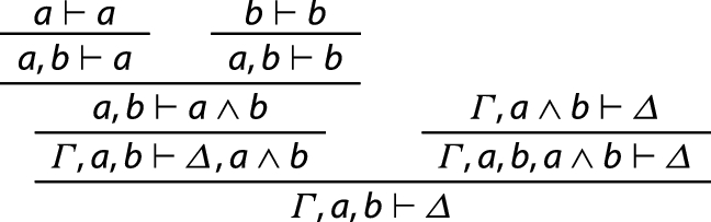
The next proposition is a sort of converse to the previous one. Let $a$ and $b$ be formulas and $\varGamma$ a finite set of formulas. The following inference rule should be called $\mathrm {Nl}(a, b)$ for brevity.

$$\frac{ \varGamma \vdash a \vee b }{ \varGamma , \lnot a \vdash b }$$

Proof

Suppose that $\mathrm {C}(a, b)$ holds. Then we also have $\mathrm {C}(\lnot b, \lnot a)$. Hence $\mathrm {Nr}(\lnot b, \lnot a)$ holds by Proposition 4. We must show that $\mathrm {Nl}(a, b)$ holds.

$\square$

Our scheme is as follows. Given a model of quantum logic, we add to Nishimura’s quantum sequent calculus all the sequents $\mathrm {C}(\,\cdot \,,\,\cdot \,)$ representing each commutative pair of physical quantities in that model. In this system, we are allowed to use the corresponding inference rules $\mathrm {Nr}(\,\cdot \,,\,\cdot \,)$ and $\mathrm {Nl}(\,\cdot \,,\,\cdot \,)$ by which we can prove many substantial theorems even in quantum logic.

5 Quantum logic programming

As stated in Sect. 1, a logic program is driven by two fundamental processes: a pattern matching process called unification and a goal rewriting process called backchaining. In this section, we present quantum versions of those processes to show how the quantum logical computation can be realized.

5.1 Unification and backchaining

In our quantum sequent calculus, the following inference rules are derived from the definition.

• i. Backchaining (I) (The positive literal case) The following derived rule holds under the condition that $\mathrm {C}(\varGamma , r)$ holds.

  $$\frac{\varGamma \vdash p_1 \wedge \dots \wedge p_m \wedge \lnot q_1 \wedge \dots \wedge \lnot q_n\ (\text {except for}\ q_k) }{ \varGamma \vdash r }\quad \quad \quad \quad (\hbox {BC (I)})$$

  where $\varGamma$ is a logic program, $\forall x_1 \in D_1 \dots \forall x_l \in D_l.(\lnot p_1 \vee \dots \vee \lnot p_m \vee q_1 \vee \dots \vee q_n)$ is a clause in $\varGamma$ and $r$ is an atomic formula that is unifiable with $q_k$.

Proof

where ? is a variable to be substituted. $\square$

To utilize Backchaining (I), find the substitution $\theta$ satisfying the equation $q_k(\,?\,)\theta \equiv r\theta$ and then apply this substitution to the whole proof diagram obtained up to that stage (this is the so-called unification). Here, a substitution $\theta$ is a function that assigns to each first-order variable $x$ a term $x\theta$.

• ii. Backchaining (II) (The negative literal case) The following derived rule holds under the condition that $\mathrm {C}(\varGamma , r)$ holds.

  $$\frac{ \varGamma \vdash p_1 \wedge \dots \wedge p_m \wedge \lnot q_1 \wedge \dots \wedge \lnot q_n\ (\text {except}\ p_k) }{ \varGamma \vdash \lnot r }\quad (\hbox {BC (II)})$$

  where $\varGamma$ is a logic program, $\forall x_1 \in D_1 \dots \forall x_l \in D_l.(\lnot p_1 \vee \dots \vee \lnot p_m \vee q_1 \vee \dots \vee q_n)$ is a clause in $\varGamma$ and $r$ is an atomic formula that is unifiable with $p_k$.

Proof

   

where ? is a variable to be substituted. $\square$

To utilize Backchaining (II), find the substitution $\theta$ satisfying the equation $p_k(\,?\,)\theta \equiv r\theta$ and then apply this substitution to the whole proof diagram obtained up to that stage.

• iii. Backchaining (III) (The positive literal case)

  $$\frac{ }{ \varGamma \vdash r }\quad \quad \quad \quad \hbox {(BC (III))}$$

  where $\varGamma$ is a logic program, $\forall x_1 \in D_1 \dots \forall x_l \in D_l.q(x)$ is a clause in $\varGamma$ and $r$ is an atomic formula that is unifiable with $q$.

Proof

where ? is a variable to be substituted. $\square$

To utilize Backchaining (III), find the substitution $\theta$ satisfying the equation $q(\,?\,)\theta \equiv r\theta$ and then apply this substitution to the whole proof diagram obtained up to that stage.

• iv Backchaining (IV) (The negative literal case)

  $$\frac{ }{ \varGamma \vdash \lnot r }\quad \hbox {(BC (IV))}$$

  where $\varGamma$ is a logic program, $\forall x_1 \in D_1 \dots \forall x_l \in D_l.\lnot p(x)$ is a clause in $\varGamma$ and $r$ is an atomic formula that is unifiable with $p$.

Proof

$$\frac{ \frac{r \vdash p(\,?\,)}{\lnot p(\,?\,) \vdash \lnot r}} {\frac{\forall x_1 \in D_1 \dots \forall x_l \in D_l.\lnot p(x) \vdash \lnot r}{\varGamma \vdash \lnot r}}$$

where ? is a variable to be substituted. $\square$

To utilize Backchaining (IV), find the substitution $\theta$ satisfying the equation $p(\,?\,)\theta \equiv r\theta$ and then apply this substitution to the whole proof diagram obtained up to that stage.

As described above, we must admit that a sort of partial commutativity is still required to allow the quantum logic version of backchainings (I) and (II) to proceed.

5.2 Proof procedure

Let $\varGamma$ be a logic program and $G$ a goal. To prove the sequent $\varGamma \vdash G$, apply $\exists$ -right if $G$ is of the form $\exists x \in D.a$, $\wedge$ -right if $G$ is of the form $a \wedge b$ and a backchaining if $G$ is an atomic formula. The choice of which backchaining to use depends on the choice of a clause in $\varGamma$. In the case where no backchaining is applicable, the proof fails at that point. In the case where more than one clause is applicable, one of the clauses is chosen indeterministically, and if this attempt fails, the proof backtracks to the last choice point to try another option.

6 An example: unification as measurement

In the previous sections, we have observed that the framework of quantum logic programming is based on the idea that a proof in quantum logic can be seen as a kind of computation. In this final section, we illustrate how this computation is interpreted in terms of quantum physics.

In quantum logic programming, an experimental context is given as a set of clauses, say, $\varGamma$, and a query is given as a goal, say, $\exists x \in D.c(x)$, which means that the proposition $c$ holds for some measurement outcome $x$. The fact that the sequent $\varGamma \vdash \exists x \in D.c(x)$ is provable means that there exists some measurement outcome $x$ that makes $c(x)$ hold in the context $\varGamma$. The specific measurement value of $x$ is obtained via unification and backchaining.

As an example, consider an experiment measuring the spins of two particles, say $A$ and $B$, along the $Z$-axis. The set $D$ of possible outcomes of this experiment is $\{\text {`up'}, \text {`down'}\}$. Now suppose that $A$ and $B$ are entangled, that is, if one has spin up then the other has spin down and vice versa:

• if $A$ has spin ‘up’ then $B$ has spin ‘down.’

• if $A$ has spin ‘down’ then $B$ has spin ‘up.’

Prior to the measurement, the quantum correlation of the pair is expressed by the set of the following clauses⁵:

• $\forall x \in D.(\lnot p(x) \vee \lnot q(x))$

• $\forall x \in D.(p(x) \vee q(x))$

Here, $p(x)$ denotes the assertion that ‘$A$ has spin $x$’ where either $x = \text {`up'}$ or $x = \text {`down.'}$ Similarly, $q(x)$ denotes the assertion that ‘$B$ has spin $x$.’ Let $\varGamma \equiv \{ \forall x\in D.(\lnot p(x) \vee \lnot q(x))$, $\forall x \in D.(p(x) \vee q(x))$(constraints on the correlation), $\forall x\in D.p(x)$(a quantity to be observed)$\}$ be a logic program and $G \equiv \exists x. (p(x) \wedge \lnot q(x))$ a goal.

The above diagram shows that $\varGamma \vdash \exists x.(p(x) \wedge \lnot q(x))$ is proved when either ‘up’ or ‘down’ is uniformly substituted for ?. This corresponds to the fact that the spins of the particles $A$ and $B$ are measured to be different (one up, and the other down) in the experimental context $\varGamma$. The computation can proceed with the help of the partial commutativity assumption in BC(II), which is automatically satisfied if we require that the observables involved be simultaneously measurable.

Under the same condition $\varGamma$, however, if the goal $G$ is permuted to $\exists x.(p(x) \wedge q(x))$, then any attempt to prove the sequent $\varGamma \vdash G$ fails. For example, the following proof is incomplete:

whether ‘up’ or ‘down’ is uniformly substituted for ?.

7 Conclusion

We formulated a feasible computational framework based on quantum logic. In this framework, the difference between quantum and classical logics was reduced to that between the inference rules for quantum and classical negations. We showed that given partial commutativity, a new rule for negation akin to the classical one is available even in the quantum case. As a result, the framework made it possible to go beyond what the usual quantum logic-based computation could do.

References

Battilotti G (2010) Interpreting quantum parallelism by sequents. Int J Theor Phys 49:3022–3029
Battilotti G (2011) Characterization of quantum states in predicative logic. Int J Theor Phys 50:3669–3681
Bowen K (1982) Programming with full first-order logic. Mach Intell 10:421–440
Bruscoli P, Guglielmi A (2003) A tutorial on proof theoretic foundations of logic programming. Lect Notes Comput Sci 2916:109–127
Dalla Chiara M L, Giuntini R (2001) Quantum logics. arXiv:quant-ph/0101028
Gallier J (1985) Logic for computer science: foundations of automatic theorem proving. Harper & Row, New York
Goldblatt R (1974) Semantic analysis of orthologic. J Philos Logic 3:19–35
Gyongyosi L, Imre S (2019) A Survey on quantum computing technology. Comput Sci Rev 31:51–71
Hardegree GM (1974) The conditional in quantum logic. Synthese 29:63–80
Miller D (1991) Uniform proofs as a foundation for logic programming. Ann Pure Appl Logic 51:125–157
Nishimura H (1980) Sequential method in quantum logic. J Symb Logic 45:339–352
Pykacz J (2000) Quantum logic as a basis for computations. Int J Theor Phys 39:839–850
Qiu DW (2004) Automata theory based on quantum logic: some characterizations. Inf Comput 109:179–195
Ying MS (2005) A theory of computation based on quantum logic(I). Theor Comput Sci 344:134–207
Ying MS (2016) Foundations of quantum programming. Morgan Kaufmann, Burlington
Ying MS, Duan RY, Feng Y, Ji ZF (2010) Predicate transformer semantics of quantum programs. In: Mackie I, Gay S (eds) Semantic techniques in quantum computation. Cambridge University Press, Cambridge, pp 311–360
Author information
Authors and Affiliations
Corresponding author
Ethics declarations
Conflicts of interest
The author declares that he has no conflict of interest.
Additional information
Publisher's Note
Springer Nature remains neutral with regard to jurisdictional claims in published maps and institutional affiliations.
Rights and permissions
About this article
Cite this article
Tokuo, K. Feasible computation based on quantum logic. SN Appl. Sci. 1, 1255 (2019). https://doi.org/10.1007/s42452-019-1193-x
Received:
Accepted:
Published:
DOI: https://doi.org/10.1007/s42452-019-1193-x