
Abstract
In this paper, we study the asymptotic behavior of an \(\varepsilon \)-periodic 3D stable structure made of beams of circular cross-section of radius \(r\) when the periodicity parameter \(\varepsilon \) and the ratio \({r/\varepsilon }\) simultaneously tend to 0. The analysis is performed within the frame of linear elasticity theory and it is based on the known decomposition of the beam displacements into a beam centerline displacement, a small rotation of the cross-sections and a warping (the deformation of the cross-sections). This decomposition allows to obtain Korn type inequalities. We introduce two unfolding operators, one for the homogenization of the set of beam centerlines and another for the dimension reduction of the beams. The limit homogenized problem is still a linear elastic, second order PDE.
1 Introduction
The aim of this work is to study the asymptotic behavior of an \(\varepsilon \)-periodic 3D stable structure made of “thin” beams of circular cross-section of radius \(r\) when the periodicity parameter \(\varepsilon \) tends to 0, in the framework of the linear elasticity. By “thin”, we mean that the radius \(r\) of the beams is much smaller than the periodicity parameter \(\varepsilon \) and that we deal with the case where \(\varepsilon \) and \(r/\varepsilon \) simultaneously tend to 0.
It is well known to engineers that for wire trusses, lattices made of very thin beams, bending dominates the stretching-compression. A contrario, if the same structures are made of thick beams the stretching-compression dominates. This is what several mathematical studies of recent decades have obtained for periodic structures made of beams. For such structures, from the mathematical point of view, this means that the processes of homogenization and dimension reduction do not commute (see the pioneer works [5, 11, 12] and also [1, 6, 8, 24, 25, 27, 28, 31]). Our aim is to investigate between these extreme cases. More precisely, we consider the case for which the ratios \(\text{diam}(\Omega )/\varepsilon \) and \(\varepsilon /r\) are of the same order (\(\Omega \) is the \(3D\) domain covered by the beam structure). In Sects. 5 and following, we show that the ratio \(r/\varepsilon ^{2}\) and its limit \(\kappa \in [0,+\infty ]\) play an important role in the estimates and the asymptotic behaviors. It worth to notice that in our analysis, \(\kappa =0\) also corresponds to the case where first the dimension reduction is done and then the homogenization, while \(\kappa =+\infty \) is for the vice-versa case. In the convergences (7.12) of Theorem 2, we show that the rescaled global displacement depends on \(\kappa \). If \(\kappa \in (0,+\infty )\), its limit is a combination of a global displacement (a pure stretching-compression) and a local bending; if \(\kappa =+\infty \) it is just a global displacement and if \(\kappa =0\) it is a local bending.
Our analysis relies on a displacement decomposition for a single beam introduced in [13,14,15]. According to those studies, a beam displacement is the sum of an elementary displacement and a warping. The elementary displacement has two components. The first one is the displacement of the beam centerline while the second stands for the small rotation of the beam cross-sections (see [13, 15]). This decomposition has been extended for structures made of a large number of beams in [14] (see [4] for the structures made of beams in the nonlinear elasticity framework). Here, similar displacement decompositions are obtained, these decompositions are used for stable beam structures (see Lemma 5) and then for periodic 3D stable structures made of beams. It is important to note that estimate (4.5)1 is the key point of this paper. It characterizes the stable structures. In a forthcoming paper, we will investigate the unstable and auxetic 3D periodic structures made of beams and we will see that all the estimates of Lemma 5 will remain except (4.5)1. These decompositions allow to obtain Korn type inequalities as well as relevant estimates of the centerline displacements.
To study the asymptotic behavior of periodic stable structures and derive limit problem we use the periodic unfolding method introduced in [9] and then developed in [10]. This method has been applied to a large number of different types of problems. We mention only a few of them which deal with periodic structures in the framework of the linear elasticity (see [3, 16,17,18,19,20,21, 26]). As general references on the theory of beams or structures made of beams, we refer to [2, 7, 22, 23, 29, 30].
The paper is organized as follows. Section 2 introduces structures made of segments and remind properties of Sobolev spaces defined on these structures. Furthermore, in this section we give a simple definition of stable and unstable structures and present several examples. In Sect. 3 we remind known results concerning the decomposition of a beam displacement into an elementary displacement and a warping. This section also gives estimates with respect to the \(L^{2}\)-norm of the strain tensor of the terms appearing in the decomposition. In Sect. 4 we extend the results of the previous section to structures made of beams. Complete estimates of our decomposition terms and Korn-type inequalities are obtained for stable structures.
In Sect. 5 we deal with an \(\varepsilon \)-periodic stable 3D structure made of \(r\)-thin beams, \({\mathcal{S}}_{\varepsilon ,r}\). For this structure we introduce a linearized elasticity problem and specify the assumptions on the applied forces. Using results from the previous section we decompose every displacement of \({\mathcal{S}}_{\varepsilon ,r}\) as the sum of an elementary displacement and a warping and provide estimates of the terms of this decomposition. The scaling of the applied forces are given with respect to \(\varepsilon \) and \(r\). That leads to an upper bound for the \(L^{2}\)-norm of the strain tensor of the solution of the elasticity problem of order 1.
In Sect. 6 we introduce different types of unfolding operators, mainly one for the centerline beams and another for the cross-sections. This last operator concerns the dimension reduction. Several results on these operators are given in this section and Appendix C.
Sect. 7, deals with the asymptotic behavior of a sequence of displacements and their strain tensors. Then, in Sect. 8, in order to obtain the limit unfolded problem we split it into three problems: the first involving the limit warpings (these fields are concentrated in the cross-sections, this step corresponds mainly to the process of dimension reduction), the second involving the local extensional and inextensional limit displacements posed on the skeleton structure and the third involving the macroscopic limit displacement posed in the homogeneous domain \(\Omega \).
In Sect. 9 we complete this analysis by giving the homogenized limit problem (Theorem 4). We obtain a linear elasticity problem with constant coefficients calculated using the correctors.
In Sect. 10 we apply the previously obtained results in the case where the periodic 3D beam structure is made of isotropic and homogeneous material. We present an approximation to the solution of the linearized elasticity problem which can be explicitly computed using the solution of the homogenized problem.
In the Appendix we give the most technical results.
2 Geometric Setting
2.1 Structures Made of Segments
In this paper we consider structures made up of a large number of segments.
Definition 1
Let \({\mathcal{S}}=\bigcup _{\ell =1}^{m}\gamma _{\ell } \), \(\gamma _{\ell } \doteq [{\mathbf{A}}^{\ell }, {\mathbf{B}}^{\ell }]\), be a set of segments and \({\mathcal{K}}\) the set of the extremities of these segments.
\({\mathcal{S}}\) is a structure if
-
\({\mathcal{S}}\) is nonincluded in a plane,
-
\({\mathcal{S}}\) is connected,
-
a common point to two segments is a common extremity of these segments,
-
if an element of \({\mathcal{K}}\) belongs to only two segments then the directions of these segments are noncollinear,
-
for every segment \(\gamma _{\ell } \) we denote \({\mathbf{t}}^{\ell }_{1}\) a unit vector in the direction of \(\gamma _{\ell } \), \(\ell \in \{1,\ldots ,m\}\).
We denote \({\mathbf{t}}_{1}\) the field belonging to \(L^{\infty }({\mathcal{S}})^{3}\) defined by
The segment \(\gamma _{\ell } \subset {\mathcal{S}}\) of length \(l _{\ell } \) is parameterized by \(S_{1}\in [0,l_{\ell } ]\), \(\ell \in \{1,\ldots ,m\}\)
The running point of \({\mathcal{S}}\) is denoted \({{\mathbf{S}}}\). For all \({{\mathbf{S}}}\in \gamma _{\ell }\) one has \({{\mathbf{S}}}={\mathbf{A}}^{\ell }+S_{1}{\mathbf{t}}^{\ell }_{1}\), \(S_{1}\in [0,l_{\ell }]\), \(\ell \in \{1,\ldots ,m\}\).
2.2 Some Reminders on the Sobolev Spaces \(L^{p}({\mathcal{S}})\) and \(H^{1}({\mathcal{S}})\)
A measurable function \(\Phi \) defined on \({\mathcal{S}}\) belongs to \(L^{p}({\mathcal{S}})\), \(p\in [1,+\infty ]\), if for every segment \(\gamma _{\ell } \subset {\mathcal{S}}\), one has \(\Phi _{|\gamma _{\ell } }\in L^{p}(\gamma _{\ell } )\), \(\ell \in \{1,\ldots ,m\}\).
For every \(\Phi \in L^{1}({\mathcal{S}})\) define
Observe that the right-hand side of the above equality does not depend on the choice of a unit vector in the directions of the segments. The space \(L^{2}({\mathcal{S}})\) is endowed with the norm
Set
where \(C({\mathcal{S}})\) is the set of continuous functions on \({\mathcal{S}}\).
For every \(\phi \in H^{1}({\mathcal{S}})\) denote
We endow \(H^{1}({\mathcal{S}})\) with the norm
2.3 Stable Structures
The space of all rigid displacements is denoted by \({\mathbf{R}}\)
We define the space \({\mathbf{U}}_{\mathcal{S}}\) as follows:
Definition 2
A structure \({\mathcal{S}}\) is a stable structure if
If the above condition is not satisfied, \({\mathcal{S}}\) is an unstable structure.
Remark 1
-
1.
The structure made of the edges of a tetrahedron is stable (see Fig. 1.a). If we remove one edge then the structure becomes unstable (see Fig. 1.b).
Fig. 1 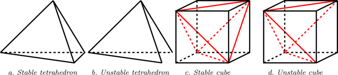
Stable and unstable structures
-
2.
The structure made of 12 edges and 6 diagonals of the faces of a cube is stable (see Fig. 1.c). If we remove one diagonal then the structure becomes unstable (see Fig. 1.d).

We equip \({\mathbf{U}}_{\mathcal{S}}\) with the following bilinear form:
and the associated semi-norm
Lemma 1
Let \({\mathcal{S}}\) be a stable structure. There exists a constant \(C\), which depends on \({\mathcal{S}}\), such that for every \(U\) in \({\mathbf{U}}_{\mathcal{S}}\) there exists \({\mathbf{r}}\in {\mathbf{R}}\) such that
Proof
Let \({\mathbf{R}}^{\perp }\) be the orthonormal of \({\mathbf{R}}\) in \({\mathbf{U}}_{\mathcal{S}}\) for the scalar product
If \(U\) belongs to \({\mathbf{R}}^{\perp }\) and satisfies \(\|U\|_{\mathcal{S}}=0\) then, since \({\mathcal{S}}\) is a stable structure, \(U\) belongs to \({\mathbf{R}}\). Therefore \(U\) is equal to 0. The semi-norm \(\|\cdot \|_{\mathcal{S}}\) is a norm on the space \({\mathbf{R}}^{\perp }\). Since \({\mathbf{R}}^{\perp }\) is a finite dimensional vector space, all the norms are equivalent. Thus (2.4) is proved. □
3 Decomposition of Beam Displacements
In this section, we remind some results concerning the decomposition of a beam displacement. These results will be used later and can be found in [15]. For the sake of simplicity these results are formulated for the beam \(B_{l,{\mathfrak{r}}}\doteq (0,l)\times D_{\mathfrak{r}}\) whose cross-sections are disc of radius \({\mathfrak{r}}\) \(({\mathfrak{r}}\leq l)\). The beam is referred to the orthonormal frame \((O;{\mathbf{e}}_{1},{\mathbf{e}}_{2},{\mathbf{e}}_{3})\) (\({\mathbf{e}}_{1}\) is the direction of the centerline). In this frame the running point is denoted \(x=(x_{1},x_{2},x_{3})\).
Any displacement \(u\in H^{1}(B_{l,{\mathfrak{r}}})^{3}\) of the beam \(B_{l,{\mathfrak{r}}}\) is uniquely decomposed as follows
where \(U^{e}\) is called elementary displacement and it stands for the displacement of the centerline of the beam and the small rotation of the cross-section at every point of the centerline (see Fig. 2):
\({\mathcal{U}}=({\mathcal{U}}_{1},{\mathcal{U}}_{2},{\mathcal{U}}_{3})\) and \({\mathcal{R}}=({\mathcal{R}}_{1},{\mathcal{R}}_{2},{\mathcal{R}}_{3})\) belong to \(H^{1}(0,l)^{3}\). The residual displacement \(\overline{u}\in H^{1}(B_{l,{\mathfrak{r}}})^{3}\) is the warping (the deformation of the cross-sections), it satisfies (for more details see [15])
Taking into account the decomposition (3.1) and the representation for the elementary displacement given by (3.2) the strain tensor \(e(u)\) has the following form:
Below is a lemma proven in [13, 15]. It gives estimates for the warping and the terms from \(U^{e}\) in the above strain tensor (3.4).

Beam \(B_{\ell ,{\mathfrak{r}}}\)
Lemma 2
Let u be in \(H^{1}(B_{l,{\mathfrak{r}}})^{3}\) decomposed as (3.1)-(3.2)-(3.3). The following estimates hold:
The constants are independent of \(l\) and \({\mathfrak{r}}\leq l\).
The function \({\mathcal{U}}\), defined in (3.1), is decomposed into the sum of two functions \({\mathcal{U}}^{h}\) and \(\overline{{\mathcal{U}}}\), where \({\mathcal{U}}^{h}\) coincides with \({\mathcal{U}}\) in the extremities of the centerline and is laffine between them (see Fig. 2), and \(\overline{{\mathcal{U}}}={\mathcal{U}}-{\mathcal{U}}^{h}\) is the residual part, i.e.,
In the same way the function ℛ, defined in (3.1), is decomposed into the sum of two functions \({\mathcal{R}}^{h}\) and \(\overline{{\mathcal{R}}}\). It is obvious, but important to note that
Lemma 3
The following estimates hold:
The constants do not depend on \(l\) and \({\mathfrak{r}}\).
Proof
Since \(\frac{d{\mathcal{R}}^{h}}{dx_{1}}\) and \(\frac{d\overline{{\mathcal{U}}}}{dx_{1}}-({ \mathcal{R}}-m({\mathcal{R}}))\wedge {\mathbf{e}}_{1}\) (\(m({ \mathcal{R}})=\frac{1}{l}\int _{0}^{l}{\mathcal{R}}(t)\, dt\)) are constant on \((0,l)\), one gets
Then, the Poincaré and the Poincaré-Wirtinger inequalities together with the above estimates yield
from which we derive the other estimates in (3.6). □
4 Decomposition of the Displacements of a Beam Structure
From now on, \({\mathcal{S}}\) is a stable structure.
The beam structure \({\mathcal{S}}_{1,{\mathfrak{r}}}\) is defined as follows:
For \(\ell \in \{1,\ldots ,m\}\), denote \({\mathcal{P}}_{\ell ,{\mathfrak{r}}}\) the straight beam with centerline \(\gamma _{\ell } =[{\mathbf{A}}^{\ell },{\mathbf{B}}^{\ell }]\) and reference cross-section the disk \(D_{\mathfrak{r}}\doteq D(O,{\mathfrak{r}})\) of radius \({\mathfrak{r}}\), \(0<{\mathfrak{r}}\leq l_{\ell } \) (the disk \(D_{1}\) for simplicity will be denoted \(D\)). The straight beam \({\mathcal{P}}_{\ell ,{\mathfrak{r}}}\) is referred to the orthonormal frame \(({\mathbf{A}}^{\ell };{\mathbf{t}}^{\ell }_{1},{\mathbf{t}}^{\ell }_{2},{\mathbf{t}}^{\ell }_{3})\)
By definition, the whole structure \({\mathcal{S}}_{1,{\mathfrak{r}}}\) contains the straight beams \({\mathcal{P}}_{\ell ,{\mathfrak{r}}}\), \(\ell \in \{1,\ldots ,m\}\) and the balls of radius \({\mathfrak{r}}\) centered in the points of \({\mathcal{K}}\), more precisely one has
The set of junction domains is denoted by \({\mathcal{J}}_{\mathfrak{r}}\). There exists \(c_{0}\) which only depends on \({\mathcal{S}}\) such that
The set \({\mathcal{J}}_{\mathfrak{r}}\) is defined in such a way that \({\mathcal{S}}_{1,{\mathfrak{r}}}\setminus \overline{{\mathcal{J}}}_{\mathfrak{r}}\) only consists of disjoint straight beams.
Definition 3
An elementary beam-structure displacement is a displacement \(U^{e}\) belonging to \(H^{1}({\mathcal{S}}_{1,{\mathfrak{r}}} )^{3}\) whose restriction to each beam is an elementary displacement and whose restriction to each junction is a rigid displacement
with \({\mathcal{U}}\) and ℛ in \(H^{1}({\mathcal{S}})^{3}\).
In [14] it is shown that every displacement \(u\in H^{1}({\mathcal{S}}_{1,{\mathfrak{r}}})^{3}\) can be decomposed as
where \(U^{e}\) is an elementary beam-structure displacement and where \(\overline{u}\in H^{1}({\mathcal{S}}_{1,{\mathfrak{r}}})^{3}\) is the warping. Here, the pair \((U^{e}, \overline{u})\) is not uniquely determined. Furthermore, the warping satisfies the conditions (3.3) “outside” the domain \({\mathcal{J}}_{\mathfrak{r}}\) (see [14, 15]), more precisely, one has
The following lemma is proved in [14, Lemma 3.4]:
Lemma 4
Let u be in \(H^{1}({\mathcal{S}}_{1,{\mathfrak{r}}})^{3}\). There exists a decomposition of \(u\), \(u = U^{e} + \overline{u}\) for which \(U^{e}\) is an elementary beam-structure displacement. The terms of this decomposition satisfy
The constants do not depend on \({\mathfrak{r}}\).
Here, again we split the field \({\mathcal{U}}\) into the sum of two fields \({\mathcal{U}}^{h}\) and \(\overline{{\mathcal{U}}}\), where \({\mathcal{U}}^{h}\) coincides with \({\mathcal{U}}\) in the nodes of \({\mathcal{S}}\) and is affine between two contiguous nodes and \(\overline{{\mathcal{U}}}={\mathcal{U}}-{\mathcal{U}}^{h}\) is the residual part.
In the same way the fields \({\mathcal{R}}^{h}\) and \(\overline{{\mathcal{R}}}\) are introduced. The field \({\mathcal{U}}^{h}\) describes the displacement of the nodes, i.e. the global behavior of the structure, whereas \(\overline{{\mathcal{U}}}\) stands for the local displacement of the beams.
By construction the fields \({\mathcal{U}}^{h}\) and \({\mathcal{R}}^{h}\) belong to \({\mathbf{U}}_{\mathcal{S}}\). Furthermore one has
Lemma 5
For every \(u\in H^{1}({\mathcal{S}}_{1,{\mathfrak{r}}})^{3}\) the following estimates hold:
Moreover, since \({\mathcal{S}}\) is a stable structure, there exists a rigid displacement \({\mathbf{r}}\in {\mathbf{R}}\), \(({\mathbf{r}}(x)={\mathbf{a}}+{\mathbf{b}}\land x)\), such that
The constants do not depend on \({\mathfrak{r}}\).
Proof
Estimates (4.4) are the immediate consequences of the Lemmas 3 and 4. Since \({\mathcal{S}}\) is a stable structure, Lemma 1 and again (4.4) yield a rigid displacement \({\mathbf{r}}\in {\mathbf{R}}\) \(({\mathbf{r}}(x)={\mathbf{a}}+{\mathbf{b}}\land x)\) such that (4.5)1 holds.
Besides, from the Poincaré-Wirtinger inequality and (4.4)4, there exists \(\widetilde{{\mathbf{b}}}\in {\mathbb{R}}^{3}\) such that
The constant does not depend on \({\mathfrak{r}}\). Then, (4.5)1 and the above estimate give
Since the structure has more than two segments with non-collinear directions, this yields
Hence, (4.5)2 is proved. □
Let \({\mathcal{S}}\) be a stable structure such that \({\mathcal{S}}\cup ({\mathcal{S}}+{\mathbf{e}}_{1})\) is a stable structure. For every displacement \(u\in H^{1}({\mathcal{S}}_{1,{\mathfrak{r}}}\cup ({\mathcal{S}}_{1,{ \mathfrak{r}}}+{\mathbf{e}}_{1}))^{3}\), Lemma 5 gives two rigid displacements \({\mathbf{r}}_{0}\), \({\mathbf{r}}_{1}\) such that
where \(G\) is the center of mass of \({\mathcal{S}}\).
Lemma 6
Let \({\mathcal{S}}\) be a stable structure such that \({\mathcal{S}}\cup ({\mathcal{S}}+{\mathbf{e}}_{1})\) is also a stable structure. The following estimate holds:
The constant does not depend on \({\mathfrak{r}}\).
Proof
From Lemma 5, there exists a rigid displacement \({\mathbf{r}}\) such that
The constant does not depend on \({\mathfrak{r}}\). Hence
The above estimates yield (4.7) since in \({\mathbf{R}}\) the norms \(\|\cdot \|_{H^{1}({\mathcal{S}})}\), \(\|\cdot \|_{H^{1}({\mathcal{S}}+{\mathbf{e}}_{1})}\) and \(\|\cdot \|_{H^{1}({\mathcal{S}}\cup ({\mathcal{S}}+{\mathbf{e}}_{1}))}\) are equivalent. □
5 A Periodic Beam Structure as 3D-Like Domain
From now on, in all the estimates, we denote by \(C\) a strictly positive constant which does not depend on \(\varepsilon \) and \(r\) .
5.1 Notations and Statement of the Problem
Below we consider periodic structures \({\mathcal{S}}\) included in a closed parallelotope.
Definition 4
A structure \({\mathcal{S}}\) is a \(3D\)-periodic structure if for every \(i\in \{1,2,3\}\) the set \({\mathcal{S}}\cup \big ({\mathcal{S}}+{\mathbf{e}}_{i} \big )\) is a structure in the sense of Definition 1.
Definition 5
A \(3D\)-periodic structure \({\mathcal{S}}\) is a \(3D\)-periodic stable structure (briefly 3-PSS) if \({\mathcal{S}}\) and \({\mathcal{S}}\cup \big ({\mathcal{S}}+{\mathbf{e}}_{i}\big )\), \(i\in \{1,2,3\}\), are stable structures in the sense of Definition 2.
Remark 2
-
1.
The structure made of 12 edges and 6 diagonals of the faces of a cube is a \(3D\)-periodic stable structure (Fig. 3.a).
Fig. 3 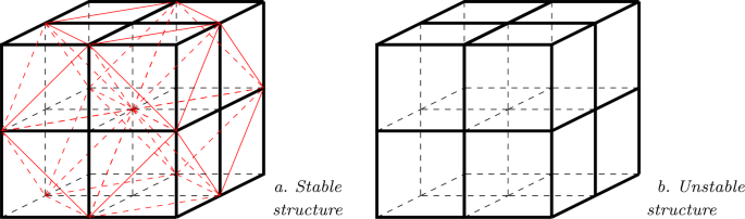
3D-periodic stable and unstable structures
-
2.
The structure made of 12 edges of a cube is not a \(3D\)-periodic stable structure (Fig. 3.b).

Let \(\Omega \) be a bounded domain in \({\mathbb{R}}^{3}\) with a Lipschitz boundary and \(\Gamma \) be a subset of \(\partial \Omega \) with nonnull measure. We assume that there exists an open set \(\Omega '\) with a Lipschitz boundary such that \(\Omega \subset \Omega '\) and \(\Omega ' \cap \partial \Omega = \Gamma \).
Denote
-
\(\Omega _{1}\doteq \big \{x\in {\mathbb{R}}^{N}\;|\; \text{dist}(x, \Omega )<1\big \}\), \(\Omega ^{int}_{\varepsilon }=\big \{x\in \Omega \;|\; \text{dist}(x,\partial \Omega )> 2\sqrt{3}\varepsilon \big \}\),
-
\(Y\doteq (0,1)^{3}\),
-
\(G=(1/2,1/2,1/2)\) the center of mass of \(Y\),
-
\({\mathcal{S}}\) a 3-periodic structure included in \(\overline{Y}\),
-
\(\Xi _{\varepsilon }\doteq \big \{\xi \in {\mathbb{Z}}^{3}\;\;|\;\;( \varepsilon \xi +\varepsilon Y)\cap \Omega \neq \emptyset \big \}\), \(\widetilde{\Xi }_{\varepsilon }\doteq \big \{\xi \in {\mathbb{Z}}^{3} \;\;|\;\;(\varepsilon \xi +\varepsilon Y)\subset \Omega \big \}\)
-
\(\Xi ^{int}_{\varepsilon }\doteq \big \{\xi \in {\mathbb{Z}}^{3}\;\;|\; \;(\varepsilon \xi +\varepsilon Y)\subset \Omega ^{int}_{\varepsilon }\big \}\),
-
\(\Xi '_{\varepsilon }\doteq \big \{\xi \in {\mathbb{Z}}^{3}\;\;|\;\;( \varepsilon \xi +\varepsilon Y)\cap \Omega '\neq \emptyset \big \}\),
-
\(\widehat{\Xi }_{\varepsilon }\doteq \big \{\xi \in \Xi _{\varepsilon }\;| \; \text{all the vertices of}\ \xi +\overline{Y}\ \text{belong to}\ \Xi _{\varepsilon }\big \}\),
-
\(\Xi _{\varepsilon ,i}\doteq \big \{\xi \in \Xi _{\varepsilon }\;|\; \xi +{\mathbf{e}}_{i} \in \Xi _{\varepsilon }\big \}\), \(i\in \{1,2,3\}\),
-
\(\Omega _{\varepsilon }\doteq \text{interior}\Big (\bigcup _{ \xi \in \Xi _{\varepsilon }}(\varepsilon \xi +\varepsilon \overline{Y}) \Big )\), \(\widehat{\Omega }_{\varepsilon }\doteq \text{interior} \Big (\bigcup _{\xi \in \widehat{\Xi }_{\varepsilon }}(\varepsilon \xi + \varepsilon \overline{Y})\Big )\), \(\Omega '_{\varepsilon }\doteq \text{interior}\Big ( \bigcup _{\xi \in \Xi '_{\varepsilon }}(\varepsilon \xi +\varepsilon \overline{Y})\Big )\)
-
\(\widehat{\Omega }^{int}_{\varepsilon }\doteq \text{interior}\Big ( \bigcup _{\xi \in \Xi ^{int}_{\varepsilon }}(\varepsilon \xi + \varepsilon \overline{Y})\Big )\), \(\widetilde{\Omega }_{\varepsilon }\doteq \text{interior} \Big (\bigcup _{\xi \in \widetilde{\Xi }_{\varepsilon }}(\varepsilon \xi +\varepsilon \overline{Y})\Big )\).
One has
The open sets \(\Omega _{\varepsilon }\), \(\Omega '_{\varepsilon }\), \(\widehat{\Omega }_{\varepsilon }\), \(\widehat{\Omega }^{int}_{\varepsilon }\) and \(\Omega ^{int}_{\varepsilon }\) are connected. Moreover, the following inclusions hold
Set
The running point of \({\mathcal{S}}_{\varepsilon }\) is denoted \({{\mathbf{s}}}\).
Let \({\mathcal{S}}_{\varepsilon ,r}\) be a beam structure consisting of balls of radius \(r\) centered on the points of \({\mathcal{K}}_{\varepsilon }\) and beams, whose cross-sections are discs of radius \(r\) and their centerlines are the segments of \({\mathcal{S}}_{\varepsilon }\)
The parametrization of the beam \({\mathcal{P}}_{\varepsilon \ell ,r}^{\xi } \) (\(\ell \in \{1,\ldots , m \}\)) is given by (see (4.1))
The junction domains (the common parts of the beams) is denoted \({\mathcal{J}}_{\varepsilon ,r}\). One has
The structure \({\mathcal{S}}_{\varepsilon ,r}\) is included in \({\Omega }_{\varepsilon }\).
The space of all admissible displacements is denoted \({\mathbf{V}}_{\varepsilon ,r}\)
It means that the displacements belonging to \({\mathbf{V}}_{\varepsilon ,r}\) “vanish” on a part \(\Gamma _{\varepsilon ,r}\) included in \(\partial {\mathcal{S}}_{\varepsilon ,r}\cap \partial \Omega \).
We assume that \({\mathcal{S}}_{\varepsilon ,r}\) is made of isotropic and homogeneous material.
For a displacement \(u\in {\mathbf{V}}_{\varepsilon ,r}\), we denote by \(e\) the strain tensor (or symmetric gradient)
We have two coordinate systems. The first one is the global Cartesian system \((x_{1},x_{2},x_{3})\) and is related to the frame \((O; {\mathbf{e}}_{1},{\mathbf{e}}_{2},{\mathbf{e}}_{3})\). The second one is the local coordinate system \((s_{1},s_{2},s_{3})\) defined for every beam and related to the frame \((\varepsilon \xi +\varepsilon {\mathbf{A}}^{\ell }_{2}; {\mathbf{t}}^{\ell }_{1},{ \mathbf{t}}^{\ell }_{2},{\mathbf{t}}^{\ell }_{3})\), \(\ell \in \{1,\ldots , m\}\). The orthonormal transformation matrix from the basis \(({\mathbf{t}}_{1}^{\ell },{\mathbf{t}}_{2}^{\ell },{\mathbf{t}}_{3}^{\ell })\) to the basis \(({\mathbf{e}}_{1},{\mathbf{e}}_{2},{\mathbf{e}}_{3})\) is \({\mathbf{T}}^{\ell }=\big ({\mathbf{t}}_{1}^{\ell }\;|\; {\mathbf{t}}_{2}^{\ell }\;|\; {\mathbf{t}}_{3}^{\ell }\big )\), this matrix belongs to \(SO(3)\).
Hence, for every displacement \(v\in H^{1}({\mathcal{P}}_{\varepsilon \ell ,r}^{\xi } )\) a straightforward calculation gives
Let \(a^{\varepsilon ,r}_{ijkl}\in L^{\infty }({\mathcal{S}}_{\varepsilon ,r})\), \((i,j,k,l)\in \{1,2,3\}^{4}\), be the components of the elasticity tensor. These functions satisfy the usual symmetry and positivity conditions
-
\(a^{\varepsilon ,r}_{ijkl}=a^{\varepsilon ,r}_{jikl}=a^{\varepsilon ,r}_{klij} \quad \text{ a.e. in } {\mathcal{S}}_{\varepsilon ,r}\);
-
for any \(\tau \in M_{s}^{3}\), where \(M_{s}^{3}\) is the space of \(3\times 3\) symmetric matrices, there exists \(C_{0}>0\) (independent of \(\varepsilon \) and \(r\)) such that
$$ a^{\varepsilon ,r}_{ijkl}\tau _{ij}\tau _{kl}\geq C_{0} \tau _{ij} \tau _{ij} \quad \text{a.e. in}\quad {\mathcal{S}}_{\varepsilon ,r}. $$(5.4)
The coefficients \(a_{ijkl}^{\varepsilon }\) are given via the functions \(a_{ijkl}\in L^{\infty }({\mathcal{S}}\times D)\)
The constitutive law for the material occupying the domain \({\mathcal{S}}_{\varepsilon ,r}\) is given by the relation between the linearized strain tensor and the stress tensor
The unknown displacement \(u_{\varepsilon }\)Footnote 1: \({\mathcal{S}}_{\varepsilon ,r}\to { \mathbb{R}}^{3}\) is the solution to the linearized elasticity system:
where \(\nu _{\varepsilon }\) is the outward normal vector to \(\partial {\mathcal{S}}_{\varepsilon ,r}\setminus \Gamma \), \(f_{\varepsilon }\) is the density of volume forces.
The variational formulation of problem (5.7) is
5.2 Final Decomposition of the Displacements of a Periodic Beam Stable Structure as a 3D-Like Domain
Let \(u\) be a displacement belonging to \({\mathbf{V}}_{\varepsilon ,r}\). As proved in [14], we can decompose \(u\) as the sum of an elementary displacement and a warping.
The decompositions introduced in Sect. 4, the estimates of Lemma 5 lead to the following estimates:
Lemma 7
For every \(u\in {\mathbf{V}}_{\varepsilon ,r}\) the following estimates hold:
Moreover, one has
Proof
We apply Lemma 5 to the structure \(\varepsilon (\xi +{\mathcal{S}}_{1,{\mathfrak{r}}})\). Replacing \({\mathfrak{r}}\) by \(\frac{r}{\varepsilon }\) and then summing over all \(\xi \in \Xi _{\varepsilon }\) give the estimates (5.9) and (5.10). □
Let \(u\) be in \(H^{1}({\mathcal{S}}_{\varepsilon ,r})^{3}\). In Lemma 5 replace \({\mathcal{S}}_{1,{\mathfrak{r}}}\) by \(\varepsilon (\xi +{\mathcal{S}}_{r/\varepsilon })\), with \(\xi \in \Xi _{\varepsilon }\), and let \({\mathbf{r}}_{\varepsilon \xi }\) be a rigid displacement given by this lemma
One has
and
Recall that if \(\xi \) belongs to \(\Xi _{\varepsilon ,i}\), the domains \(\varepsilon (\xi +{\mathcal{S}}_{r/\varepsilon })\) and \(\varepsilon (\xi +{\mathbf{e}}_{i} +{\mathcal{S}}_{r/\varepsilon })\), \(i\in \{1,2,3\}\), are included in \({\mathcal{S}}_{\varepsilon ,r}\). Then, applying estimates (4.7) in Lemma 6 to the structure \(\varepsilon (\xi +{\mathcal{S}}_{r/\varepsilon })\) we obtain
Set

Now, define
-
 (resp.
  ) in the cell \(\varepsilon (\xi +\overline{Y})\), \(\xi \in \widehat{\Xi }_{\varepsilon }\), as the \(Q_{1}\) interpolate of its values on the vertices of this parallelotope.
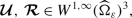
-
\({\mathbf{a}}\) (resp. \({\mathbf{b}}\)) as a piecewise constant function, equals to \({\mathbf{a}}(\varepsilon \xi )\) (resp. \({\mathbf{b}}(\varepsilon \xi )\)) in the cell \(\varepsilon (\xi + Y)\), \(\xi \in \Xi _{\varepsilon }\).
$$ {\mathbf{a}},\;{\mathbf{b}}\in L^{\infty }(\Omega _{\varepsilon })^{3}. $$(5.14)
 (resp.
  ) in the cell
We remind the following classical results ([10, Lemmas 5.22 and 5.35] and [16, Lemmas 5.2 and 5.3]):
Lemma 8
Let \(\Omega \) be a bounded domain in \({\mathbb{R}}^{N}\) with Lipschitz boundary. There exists \(\delta _{0}>0\) such that for all \(\delta \in (0,\delta _{0}]\) the sets \(\Omega _{\delta }^{int}=\big \{x\in \Omega \;|\; \operatorname{dist}(x, \partial \Omega )> \delta \big \}\) are uniformly Lipschitz.
Lemma 9
Let \(\Psi \) be a function defined on \(\Xi _{\varepsilon }\) and extended using the classical \(Q_{1}\) interpolation procedure in a function denoted \(\Psi \) and belonging to \(W^{1,\infty }(\widehat{\Omega }_{\varepsilon })\) then we have
Proposition 1
Let \({\mathcal{S}}\) be a 3-PSS. For every displacement \(u\in H^{1}({\mathcal{S}}_{\varepsilon ,r})^{3}\), one has

Moreover, there exists a rigid displacement \({\mathbf{r}}\) such that

Proof
The estimates (5.13)1,2 and Lemma 9 yield

And (5.16)1,2 are proved. From which we get

which also read (5.16)3. Lemma 8 allows to apply the 3D-Korn inequality in the domain \(\Omega ^{int}_{\varepsilon }\) using estimate (5.16)3. That gives (5.17). □
Proposition 2
Let \({\mathcal{S}}\) be a 3-PSS. For every \(u\) in \({\mathbf{V}}_{\varepsilon ,r}\), the following estimates of the elementary displacement holds:
Moreover, one has the Korn type inequalities
Proof
This proposition is a consequence of Proposition 1 and two lemmas postponed in Appendix A. □
5.3 Assumptions on the Applied Forces
We distinguish two types of applied forces. The first ones are applied in the beams (between the junctions) and the second ones are applied in the junctions.
⋆ The applied forces \({\mathbf{f}}_{\varepsilon }\) in the set of beams \(\bigcup _{\xi \in \Xi _{\varepsilon }} \bigcup _{\ell =1}^{m} {\mathcal{P}}_{\varepsilon \ell ,r}^{\xi } \).
For simplicity, we choose these applied forces constant in the cross-sections and equal to
⋆ The applied forces \(F_{r,{\mathcal{K}}_{\varepsilon }}\) in the junctions.
These forces are defined in the balls centered in the nodes with radius \(r\)
Lemma 10
Taking the applied forces as
where \(({\mathbf{f}},\,F,\,G)\in \big (C(\overline{\Omega })^{3}\big )^{3}\) and where \({\mathbf{1}}_{{\mathcal{O}}}\) is the characteristic function of the set \({\mathcal{O}}\), we obtain
Proof
The proof is postponed in Appendix B. □
As a consequence of the above lemma one obtains
Proposition 3
The solution \(u_{\varepsilon }\) to the problem (5.8) satisfies
Proof
In order to obtain apriori estimate of \(u_{\varepsilon }\), we test (5.8) with \(v=u_{\varepsilon }\). From (5.21), we obtain
which leads to (5.22). □
6 The Unfolding Operators
The classical unfolding operator \({\mathcal{T}}_{\varepsilon }\) is developed in [9, 10]. Here, we will use similar operators \({\mathcal{T}}^{ext}_{\varepsilon }\), \({\mathcal{T}}^{\mathcal{S}}_{\varepsilon }\), \({\mathcal{T}}^{b,\ell }_{\varepsilon }\) in the context of the domains \(\Omega _{\varepsilon }\), \({\mathcal{S}}_{\varepsilon }\) and \({\mathcal{S}}_{\varepsilon ,r}\).
Definition 6
(Classical unfolding-operator)
For a measurable function \(\phi \) on \(\Omega \), the unfolding operator \({\mathcal{T}}_{\varepsilon }\) is defined as follows:
Definition 7
(Unfolding-operator)
For a measurable function \(\phi \) on \(\Omega _{\varepsilon }\), the unfolding operator \({\mathcal{T}}^{ext}_{\varepsilon }\) is defined as follows:
Lemma 11
Let \(\phi \) be in \(L^{p}(\Omega _{\varepsilon })\), \(p\in [1,+\infty )\). One has
where
Proof
Inequality (6.1) is an immediate consequence of the definitions of these operators. □
As a consequence of the above lemma, the properties of the operator \({\mathcal{T}}^{ext}_{\varepsilon }\) are similar to those of the classical unfolding operator \({\mathcal{T}}_{\varepsilon }\). For the main properties of the unfolding operator \({\mathcal{T}}_{\varepsilon }\), we refer the reader to [10, Chap. 1].
Below, we introduce two new unfolding operators. The first one is used for the centerlines of beams and the second one is used for the small beams (it concerns the reduction of dimension).
In the definitions below, \(\varepsilon \Big [\frac{x}{\varepsilon }\Big ]\) represents a macroscopic coordinate (the same coordinate for all the points in the cell \(\varepsilon \Big [\frac{x}{\varepsilon }\Big ]+ \varepsilon Y\) ) while \({{\mathbf{S}}}\) is the coordinate of a point belonging to \({\mathcal{S}}\) . Hence, \(\varepsilon \Big [\frac{x}{\varepsilon }\Big ]+ \varepsilon {{\mathbf{S}}}\) represents the coordinate of a point belonging to \({\mathcal{S}}_{\varepsilon }\) . In order to get a map \((x,{{\mathbf{S}}})\longmapsto \varepsilon \Big [\frac{x}{\varepsilon }\Big ]+\varepsilon {{\mathbf{S}}}\) almost one to one, we have to restrict the set \({\mathcal{S}}\) . This is why from now on, to introduce the unfolding operator, in lieu of \({\mathcal{S}}\) we consider the set
For simplicity we still refer to it as \({\mathcal{S}}\) . The set of new nodes is always denoted \({\mathcal{K}}\) and the number of beams of \({\mathcal{S}}\) is still denoted \(m\) .
Definition 8
(Centerlines unfolding)
For a measurable function \(\phi \) on \({\mathcal{S}}_{\varepsilon }\), the unfolding operator \({\mathcal{T}}^{\mathcal{S}}_{\varepsilon }\) is defined as follows:
Definition 9
(Beams unfolding)
For a measurable function \(u\) on \({\mathcal{S}}_{\varepsilon ,r}\), the unfolding operator \({\mathcal{T}}^{b,\ell }_{\varepsilon }\) is defined as follows \((\ell \in \{1,\ldots ,m\})\):
where \(\widehat{S}=(S_{1},S_{2},S_{3})\), \({\mathbf{A}}^{\ell }\) is an extremity of the segment \(\gamma _{\ell } \subset {\mathcal{S}}\) and \(D=D_{1}\) is the disc of radius 1.
Let \(\phi \) be measurable on \({\mathcal{S}}_{\varepsilon }\), one has
Lemma 12
(Properties of the operators \({\mathcal{T}}^{\mathcal{S}}_{\varepsilon }\) and \({\mathcal{T}}^{b,\ell }_{\varepsilon }\))
For every \(\phi \in L^{1}({\mathcal{S}}_{\varepsilon })\)
For every \(\phi \in L^{2}({\mathcal{S}}_{\varepsilon })\)
For every \(\phi \) in \(H^{1}({\mathcal{S}}_{\varepsilon })\)
For every \(\psi \) in \(L^{2}({\mathcal{S}}_{\varepsilon ,r})\)
For every \(\psi \) in \(L^{1}({\mathcal{S}}_{\varepsilon ,r})\)
The constant only depends on \({\mathcal{S}}\).
For every \(u\) in \(H^{1}({\mathcal{S}}_{\varepsilon ,r})\) (\(j\in \{2,3 \}\) and \(\ell \in \{1,\ldots ,m\}\))
Proof
We prove (6.2) and (6.3). Let \(\phi \) be in \(L^{1}({\mathcal{S}}_{\varepsilon })\)
We prove (6.6). For \(u \in L^{1}({\mathcal{S}}_{\varepsilon ,r})\) we have
Now, replacing \(\varepsilon \xi +\varepsilon {\mathbf{A}}^{\ell }+\varepsilon S_{1}{\mathbf{t}}^{\ell }_{1}+rS_{2}{\mathbf{t}}^{\ell }_{2}+rS_{3}{\mathbf{t}}^{\ell }_{3}\) by \(x\) and taking into account that the matrix \(({\mathbf{t}}_{1}^{\ell }|{\mathbf{t}}_{2}^{\ell }|{\mathbf{t}}_{3}^{\ell })\) belongs to \({SO}(3)\), we obtain
and (6.6) follows.
Properties (6.4)-(6.7) are direct consequences of the definitions of the unfolding operators. □
Corollary 1
For every \(\phi \) in \(L^{2}({\mathcal{S}}_{\varepsilon })\), \(\ell \in \{1,\ldots ,m\}\)
From now on, every function belonging to \(L^{p}(\Omega )\) (\(p \in [1,+\infty ]\)) will be extended by 0 in \(\Omega _{\varepsilon }\setminus \overline{\Omega }\).
Denote \(Q_{1}(Y)\) the subspace of \(W^{1,\infty }(Y)\) containing the functions which are the \(Q_{1}\) interpolations of their values at the vertices of the parallelotope \(\overline{Y}\).
Lemma 13
For every \(\Phi \) in \(W^{1,\infty }(\Omega _{\varepsilon })\) satisfying
Then \(\Phi _{|{\mathcal{S}}_{\varepsilon }}\) belongs to \(W^{1,\infty }({\mathcal{S}}_{\varepsilon })\) and it satisfies
Let \(\{\Phi _{\varepsilon }\}_{\varepsilon }\) be a sequence of functions belonging to \(W^{1,\infty }(\Omega _{\varepsilon })\) satisfying (6.9) and
then, up to a subsequence of \(\{\varepsilon \}\), there exists \(\Phi \in L^{2}(\Omega )\) such that
Moreover, if one also has
then \(\Phi \) belongs to \(H^{1}(\Omega )\) and
Proof
The proof is given in Appendix C. □
First convergence results for sequences in \(H^{1}({\mathcal{S}}_{\varepsilon })\).
Lemma 14
Let \(\{\phi _{\varepsilon }\}_{\varepsilon }\) be a sequence of functions belonging to \(H^{1}({\mathcal{S}}_{\varepsilon })\) satisfying
Then, up to a subsequence, there exists \(\widehat{\phi }\in L^{2}(\Omega ; H^{1}_{per}({\mathcal{S}}))\) such that
If we only have
then, up to a subsequence, there exists \(\widehat{\phi }\in L^{2}(\Omega ; H^{1}_{per}({\mathcal{S}}))\) such that
Proof
The proof is postponed in Appendix C. □
Definition 10
The local average operator \({\mathcal{M}}^{*}_{\varepsilon }\) is defined from \(L^{2}({\mathcal{S}}_{\varepsilon })\) to \(L^{2}(\Omega _{\varepsilon })\) as
By convention the value of \({\mathcal{M}}^{*}_{\varepsilon }(\phi )\) on the cell \(\varepsilon (\xi +Y)\) is simply denoted \({\mathcal{M}}^{*}_{\varepsilon }(\phi )(\varepsilon \xi )\).
A second lemma for sequences in \(H^{1}({\mathcal{S}}_{\varepsilon })\).
Lemma 15
Let \(\{\phi _{\varepsilon }\}_{\varepsilon }\) be a sequence of functions belonging to \(H^{1}({\mathcal{S}}_{\varepsilon })\) satisfying
Then, up to a subsequence, there exists \((\Phi ,\widehat{\phi })\in H^{1}(\Omega )\times L^{2}(\Omega ; H^{1}_{per}({ \mathcal{S}}))\) such that
Proof
The proof is postponed in Appendix C. □
Denote
Corollary 2
Let \(\{\phi _{\varepsilon }\}_{\varepsilon }\) be a sequence of functions belonging to \(H^{1}({\mathcal{S}}_{\varepsilon })^{3}\cap {\mathbf{V}}_{\varepsilon ,r}\) and satisfying the following
Then, up to a subsequence, there exists \((\Phi ,\widehat{\phi })\in H^{1}_{\Gamma }(\Omega )^{3} \times L^{2}( \Omega ; H^{1}_{per}({\mathcal{S}}))^{3}\) such that
Proof
Since \(\{\phi _{\varepsilon }\}_{\varepsilon }\) belongs to \(V_{\varepsilon ,r}\), these functions equal to 0 in \({\mathcal{S}}'_{\varepsilon }\setminus {\mathcal{S}}_{\varepsilon }\). Applying Lemma 15 with \({\mathcal{S}}'_{\varepsilon }\) instead \({\mathcal{S}}_{\varepsilon }\) and with \(\Omega '\) instead \(\Omega \) give the result. □
7 Asymptotic Behaviors
7.1 Asymptotic Behavior of a Sequence of Displacements
From now on, we assume that \(r\) is a function of \(\varepsilon \) satisfying the following conditions:
In addition, every field appearing in the decomposition introduced in the previous sections will be denoted with only the index \(\varepsilon \).
In this section we consider a sequence \(\{u_{\varepsilon }\}_{\varepsilon }\) of displacements belonging to \({\mathbf{V}}_{\varepsilon ,r}\) and satisfying
Theorem 1
For a subsequence of \(\{\varepsilon \}\), still denoted \(\{\varepsilon \}\), one has
(i) there exist \({\mathcal{U}}\in {H^{1}_{\Gamma }(\Omega )}^{3}\), \(\overline{{\mathcal{U}}}\in {L^{2}(\Omega ;H^{1}_{per}({ \mathcal{S}}))}^{3}\) such that \(S\longmapsto \overline{{\mathcal{U}}}(\cdot , S)\land {\mathbf{t}}_{1}\) is an affine function on every segment of \({\mathcal{S}}\) and the following convergences hold:

where \(e({\mathcal{U}})\) is the symmetric gradient of the displacement \({\mathcal{U}}\)
(ii) there exists \(\widehat{{\mathcal{U}}}\in L^{2}(\Omega ; H^{1}_{per}({\mathcal{S}}))^{3}\) such that \(\widehat{{\mathcal{U}}}_{|\gamma _{\ell } }\in L^{2}(\Omega ; H^{1}_{0}( \gamma _{\ell }) \cap H^{2}(\gamma _{\ell }))^{3}\), \(\widehat{{\mathcal{U}}}_{|\gamma _{\ell } }\cdot {\mathbf{t}}^{\ell }_{1}=0\), \(\ell \in \{1,\ldots ,m\}\) and
(iii) there exists \({\mathcal{Z}}\in L^{2}(\Omega \times {\mathcal{S}})^{3}\) such that
(iv) there exists \(\widehat{{\mathcal{R}}}\in L^{2}(\Omega ;H^{1}_{per}({\mathcal{S}}))^{3}\) such that
and
(v) there exists \(\overline{u}\in L^{2}(\Omega \times {\mathcal{S}};H^{1}(D))^{3}\) such that
Proof
Below, every convergence is up to a subsequence of \(\{\varepsilon \}\) still denoted \(\{\varepsilon \}\).
(i) From Lemma 21 and Proposition 3 we have the following estimates:

Lemma 5.1 in [16] gives a field \({\mathcal{U}}\in H^{1}_{\Gamma }(\Omega )^{3}\) such that (7.2)1,2 hold.
From the estimates (5.10) and (A.2) one obtains
Hence, the convergences (7.2)3,4 are the consequences of Corollary 2.
Since
the convergence (7.2)5 holds (observe that \((\nabla {\mathcal{U}}\,{\mathbf{t}}_{1})\cdot {\mathbf{t}}_{1}=(e({ \mathcal{U}})\,{\mathbf{t}}_{1})\cdot {\mathbf{t}}_{1}\)).
(ii) From (5.10), (5.22), (1) and the fact that by construction \(\overline{{\mathcal{U}}}_{\varepsilon |\gamma _{\ell } }(0)= \overline{{\mathcal{U}}}_{\varepsilon |\gamma _{\ell } }(\varepsilon l_{ \ell } )=0\), we obtain
Thus, up to a subsequence, there exists \(\widehat{{\mathcal{U}}}\in {L^{2}(\Omega ;H^{1}({\mathcal{S}}))}^{3}\) such that \(\widehat{{\mathcal{U}}}_{|\gamma _{\ell } }\in L^{2}(\Omega ;H^{1}_{0}( \gamma _{\ell }))^{3}\), \(\widehat{{\mathcal{U}}}_{|\gamma _{\ell } }\cdot {\mathbf{t}}^{\ell }_{1}=0\), \(\ell \in \{1,\ldots ,m\}\) and convergence \(\text{(7.3)}_{1}\) holds.
(iii) Estimates (5.9)4-(5.10) and (6.2) yield
Then, there exists a field \({\mathcal{Z}}\in L^{2}(\Omega \times {\mathcal{S}})^{3}\) such that
and by (7.2)4 we have
(iv) Estimate (5.18)2 gives
Thus, up to a subsequence, there exists a function \(\widehat{{\mathcal{R}}}\in L^{2}(\Omega ; H^{1}_{per}({ \mathcal{S}}))^{3}\) (see Lemma 14) such that (7.5) holds.
On the one hand, from (7.9) we have
On the other hand from convergences (7.3)1, (7.5) we obtain
Hence, we obtain (7.6) and
Then \(\widehat{{\mathcal{U}}}_{|\gamma _{\ell } }\in {L^{2}(\Omega ;H^{1}_{0}( \gamma _{\ell }) \cap H^{2}(\gamma _{\ell }) )}^{3}\).
(v) Taking into account (5.9)1,2, (6.7)2 and (6.5) for \(j=2,3\), \(\ell \in \{1,\ldots ,m\}\), we have
Hence, up to a subsequence, there exists \(\overline{u}\in {L^{2}(\Omega \times {\mathcal{S}};H^{1}(D))}^{3}\) such that (7.7)1 holds.
In order to show convergence (7.7)2, note that from (5.9)2, (6.7)1 and (6.5) it follows
Therefore, convergence \(\text{(7.7)}_{2}\) is proved, since
□
Remark 3
Due to (4.2), the warping \(\overline{u}\) satisfies
Denote

The field \(\overline{{\mathcal{U}}}\) is in  while the pair \(\big (\widehat{{\mathcal{U}}},\widehat{{\mathcal{R}}}\big )\) belongs to
  . It worth to notice that a field \(\overline{{\mathcal{A}}}\) belonging to \(H^{1}_{per,0}({\mathcal{S}})^{3}\) is a local extensional displacement if and only if
for all \(\widehat{{\mathcal{A}}}\in H^{1}_{per}({\mathcal{S}})^{3}\) which is the first component of an element belonging to  .
.
We endow  (resp.
  ) with the semi-norm

Lemma 16
On  the semi-norm \(\|\cdot \|_{{\mathcal{S}}}\) is a norm equivalent to the norm of \(H^{1}({\mathcal{S}})^{3}\). On
  the semi-norm
  is a norm equivalent to the norm of \(H^{1}({\mathcal{S}})^{3}\times H^{1}({\mathcal{S}})^{3}\).
Proof
The proof is given in Appendix D. □
7.2 Asymptotic Behavior of the Strain Tensor
For every \({\mathcal{V}}\in {H^{1}_{\Gamma }(\Omega )}^{3}\),  and \(\widetilde{v}\in L^{2}(\Omega \times {\mathcal{S}};H^{1}(D))^{3}\) we define the symmetric tensors ℰ, \({\mathcal{E}}_{{\mathcal{S}}}\), \({\mathcal{E}}_{D}\) by
Theorem 2
Let \(u_{\varepsilon }\) be the solution to (5.8). There exist a subsequence of \(\{\varepsilon \}\), still denoted \(\{\varepsilon \}\), and \({\mathcal{U}}\in H^{1}_{\Gamma }(\Omega )^{3}\),  and \(\widetilde{u}\in L^{2}(\Omega \times {\mathcal{S}};H^{1}(D))^{3}\) such that the following convergences hold (\(\ell \in \{1,\ldots ,m\}\)):
and
Proof
Below, we give the asymptotic behavior of the sequence \(\{{\mathcal{T}}^{b,\ell }_{\varepsilon }(u_{\varepsilon })\}\) as \(\varepsilon \to 0\) and \(r/\varepsilon \to 0\). One has
From (7.7)1 we have (\(\ell \in \{1,\ldots ,m\}\))
From Definition 3 we have (\(\ell \in \{1,\ldots ,m\}\))
The convergences (7.2)3, (7.3), (7.5) yield
if \(\kappa =0\), from (7.3) we obtain
Hence, the convergences (7.12) hold.
Now we consider the asymptotic behavior of the strain tensors \({\mathcal{T}}^{b,\ell }_{\varepsilon }(e_{s}(u_{\varepsilon }))\)
From (7.7), we obtain \((\ell \in [1,\ldots,m])\)
Next from the convergences (7.2)4, (7.3)2, (7.5) and (7.6) we obtain
We set
Hence, one has
and (7.13) holds. □
Denote

Thanks to the conditions (7.11) satisfied by \(\overline{u}\) and the definition of \(\widetilde{u}\), one obtains

For the sake of simplicity, if \(\widetilde{v}\) belongs to \(L^{2}(\Omega \times {\mathcal{S}}; H^{1}(D)^{3})\) and is such that

we will write that \(\widetilde{v}\) belongs to  .
.
8 The Limit Unfolded Problem
To obtain the limit unfolded problem, we will choose test displacements \(v\) in \({\mathbf{V}}_{\varepsilon ,r}\) which vanish in the junction domain \({\mathcal{J}}_{\varepsilon ,r}\) or which are equal to rigid displacements in \({\mathcal{J}}_{\varepsilon ,r}\). In doing so, we will have
The step-by-step construction of the unfolded limit problem (8.12) is considered in Lemmas 17, 18, 19.
Lemma 17
(The limit problem involving the limit warping)
For every \(\ell \in \{1,\ldots ,m\}\) one has
Proof
Set
where \(W\in {\mathcal{D}}(\Omega )\), \(V \in {\mathcal{D}}(\gamma _{\ell })\) and \(\varphi \in {H^{1}(D)}^{3}\), \(\ell \in \{1,\ldots , m\}\). Since \(V\) belongs to \({\mathcal{D}}(\gamma _{\ell })\) and \(r/\varepsilon \) goes to 0, the support of the above test-displacement is only included in the beams whose centerline is \(\varepsilon \xi +\varepsilon \gamma _{\ell }\). Moreover, this displacement vanishes in the neighborhood of the extremities of this beam, it means that this displacement vanishes in the junction domain \({\mathcal{J}}_{\varepsilon ,r}\).
One has
We apply the unfolding operator \({\mathcal{T}}^{b,\ell }_{\varepsilon }\) and pass to the limit, this gives
Hence
Using (5.20) and then unfolding and passing to the limit yield
The above convergences lead to
Finally, since the space \({\mathcal{D}}(\Omega )\otimes {\mathcal{D}}(\gamma _{\ell })\otimes {H^{1}(D)}^{3}\) is dense in \({L^{2}(\Omega \times \gamma _{\ell };H^{1}(D))}^{3}\) we obtain (8.1). □
Lemma 18
(The limit problem involving the extensional and inextensional limit displacements)
One has

Proof
Let \(\phi \) be in \({\mathcal{D}}(\Omega )\) and \((\overline{{\mathcal{V}}},\widehat{{\mathcal{V}}}, \widehat{{\mathcal{B}}})\) in  such that \(\overline{{\mathcal{V}}}\) and \((\widehat{{\mathcal{V}}},\widehat{{\mathcal{B}}})\) are constant in the neighborhood of every node of \({\mathcal{S}}\).
Step 1. The test displacement.
Set
where \(\phi _{\varepsilon ,r}\) is defined in Appendix F. Since the above fields are constant in the neighborhood of every node of \({\mathcal{S}}_{\varepsilon }\), this allows to extend them in functions belonging to \(H^{1}({\mathcal{S}}_{\varepsilon ,r})\). Hence, these functions are constant in the cross-sections and in the neighborhood of every node. We remind (see Appendix F)
We define \(v_{\varepsilon ,r}\) in the beam whose centerline is \(\varepsilon \xi +\varepsilon \gamma _{\ell }\), \(\ell \in \{1,\ldots ,m\}\) by
Observe that for every \(x\) in \(B(\varepsilon \xi +\varepsilon A^{\ell }, c_{0}r)\cap {\mathcal{S}}_{ \varepsilon ,r}\) one has
Hence, \(v_{\varepsilon ,r}\) is a rigid displacement in \(B(\varepsilon \xi +\varepsilon A^{\ell }, c_{0}r) \cap {\mathcal{S}}_{ \varepsilon ,r}\). This test displacement belongs to \({\mathbf{V}}_{\varepsilon ,r}\).
Step 2. Limit of the LHS.
One has
Observe that \(\frac{\partial v_{\varepsilon ,r}}{\partial s_{2}} \cdot {\mathbf{t}}_{2}=\frac{\partial v_{\varepsilon ,r}}{\partial s_{3}} \cdot {\mathbf{t}}_{3}=\frac{\partial v_{\varepsilon ,r}}{\partial s_{2}} \cdot {\mathbf{t}}_{3}+\frac{\partial v_{\varepsilon ,r}}{\partial s_{3}} \cdot {\mathbf{t}}_{2}=0\) and by definition of  , one has \(\widehat{{\mathcal{V}}}\cdot {\mathbf{t}}_{1}=0\).
The convergences (8.6) yield
The presence of \(\widetilde{v}_{\varepsilon ,r}\) in the test displacement is just to eliminate \(\frac{\varepsilon ^{3}}{r^{2}}\frac{d\phi _{\varepsilon ,r} }{ds_{1}}\widehat{{\mathcal{V}}}\Big (\frac{\cdot }{\varepsilon } \Big )\cdot {\mathbf{t}}^{\ell }_{\alpha }\) in \(\frac{\partial v_{\varepsilon ,r}}{\partial s_{i}} \cdot {\mathbf{t}}^{\ell }_{1}+ \frac{\partial v_{\varepsilon ,r}}{\partial s_{1}}\cdot {\mathbf{t}}^{\ell }_{i}\), \(i\in \{2,3\}\). Then, again using the convergences (8.6), we obtain
Hence,
where
Unfolding the left-hand side of (5.8) and passing to the limit give
Step 3. Limit of the RHS.
Now, we consider the right-hand side of (5.8)
Let’s take the first term in the right-hand side of (8.8). Taking into account the symmetries of the ball \(B(\varepsilon \xi +\varepsilon A^{\ell }, r)\) and the fact that \(\int _{B(O , r)}|x|^{2}\,dx=\frac{4\pi r^{5}}{5}\). After a straightforward calculation, one obtains
Since \(|Y|=1\), one has
Hence,
Now, we take the second term in the right-hand side of (8.8).
Due to (6.6), we only need to consider \(\frac{r^{2}}{\varepsilon ^{2}}\sum _{\ell =1}^{m}\, \int _{\Omega \times \gamma _{\ell } \times D}{\mathcal{T}}^{b,\ell }_{\varepsilon }({\mathbf{f}}_{\varepsilon })\cdot {\mathcal{T}}^{b,\ell }_{\varepsilon }(v_{\varepsilon ,r})\,\,dx\,d\widehat{S}\). One has
Assumptions (7.1) and convergence (8.6)1 lead to
Hence,
Lemma 24 and the density of  in
in  and
and  in
in  lead to

Besides, since \(\widetilde{\overline{v}}\) belongs to \(L^{2}(\Omega \times {\mathcal{S}}; H^{1}(D))^{3}\) equality (8.1) together with the one above yield (8.5). □
Lemma 19
(The limit problem involving the macroscopic limit displacement)
One has
whereFootnote 2\(|{\mathcal{K}}|\) is the number of points of \({\mathcal{K}}\) and \({\mathcal{S}}\) the measure of \({\mathcal{S}}\).
Proof
Step 1. Limit of the LHS of (5.8).
Let \({\mathcal{V}}\) be in \({\mathcal{D}}({\mathbb{R}}^{3})^{3}\) such that \({\mathcal{V}}=0\) in \(\Omega '\setminus \overline{\Omega }\). We define \({\mathcal{V}}_{\varepsilon ,r}\) using F. This function is extended as in Step 1 of the proof of Lemma 18. Set
We have
where
Convergence (8.11) leads to
Step 2. Limit of the RHS.
Now we consider the right-hand side of (5.8). By (5.20), firstly we have
and secondly, due to (6.6), we pass to the limit in
Hence
Since the set of functions belonging to \({\mathcal{D}}({\mathbb{R}}^{3})^{3}\) and vanishing in \(\Omega '\setminus {\Omega }\) is dense in \(H^{1}_{\Gamma }(\Omega )^{3}\), we obtain
Taking into account that \(\widetilde{\widetilde{v}}\) belongs to \(L^{2}(\Omega \times {\mathcal{S}}; H^{1}(D))^{3}\) and using (8.1), equality (8.10) is proved. □
Theorem 3
(The unfolded limit problem)
Let \(u_{\varepsilon }\) be the solution to (5.8). There exist \({\mathcal{U}}\in H^{1}_{\Gamma }(\Omega )^{3}\),  and
and  such that \(\big ({\mathcal{U}},\overline{{\mathcal{U}}}, \widehat{{\mathcal{U}}},\widehat{{\mathcal{R}}},\widetilde{u} \big )\) is the solution to the following unfolded problem:

Moreover, the following convergences hold (\(\ell \in \{1,\ldots ,m\}\)):
Denote
Proof
From Lemmas 17, 18, 19 we obtain that \(({\mathcal{U}}, \overline{{\mathcal{U}}}, \widehat{{\mathcal{U}}},\widehat{{\mathcal{R}}},\widetilde{u})\) satisfies (8.12) for every test function \({\mathcal{V}}\in H^{1}_{\Gamma }(\Omega )^{3}\),  and
and  .
.
The coercivity of this problem is given by Lemma 26. Since the problem (8.12) admits a unique solution, the whole sequences in Theorems 1, 2 and (8.13) converge to their limits.
Now, we prove the strong convergence (8.13). First, observe that due to the inclusion of \({\mathcal{J}}_{\varepsilon ,r}\) in \(\bigcup _{A\in {\mathcal{K}}_{\varepsilon }} B(A,c_{0}r)\) given by (5.1), the portions of beams which correspond to \(S_{1}\in (2c_{0} r,l_{\ell }- 2c_{0} r)\) are all disjoint. Furthermore, since \(\sigma (u_{\varepsilon }):e(u_{\varepsilon })\) is non-negative, one has
From (7.13) and the fact that \(r\) goes to 0, one obtains (\(\ell \in \{1,\ldots ,m\}\))
Hence, choosing \(u_{\varepsilon }\) as a test function in (5.8) and using a weak lower semi-continuity of convex functionals, one has
Thus, all inequalities above are equalities and
which in turn leads to the strong convergence (8.13). □
9 The Homogenized Problem
9.1 Expression of the Warping \(\widetilde{u}\)
In this subsection we give the expression of the warping \(\widetilde{u}\) in terms of the macroscopic displacement \({\mathcal{U}}\) and the microscopic fields \(\overline{\mathcal{U}}\), \(\widehat{\mathcal{U}}\), \(\widehat{\mathcal{R}}\).
To this end, we use the variational formulation (8.1). For every \(\ell \in \{1,\ldots ,m\}\) one has

This shows that \(\widetilde{u}\) can be expressed in terms of the elements of the tensors ℰ and \({\mathcal{E}}_{\mathcal{S}}\).
We write
Now, we introduce 4 correctors which are the solutions to the following cell problems:

Since \(a_{ijkl}\)’s belong to \(L^{\infty }({\mathcal{S}}\times D)\), then  , \(q\in \{1, \ldots , 4\}\).
Hence, we have
9.2 Expression of the Microscopic Fields \(\overline{\mathcal{U}}\), \(\widehat{\mathcal{U}}\), \(\widehat{\mathcal{R}}\)
In this subsection we give the expression of the microscopic fields \(\overline{\mathcal{U}}\), \(\widehat{\mathcal{U}}\), \(\widehat{\mathcal{R}}\) in terms of the macroscopic displacement \({\mathcal{U}}\). To this end, as before, we use the variational formulation (8.12).
Thus, taking \({\mathcal{V}}=0\), \(\widetilde{v}=0\) in (8.12), then replacing \(\widetilde{u}\) by its expression, using the following equality:
together with (9.1) give

We write
and the variational problem (9.3) has the following form:

where the symmetric matrix \(\mathfrak{A}\) belongs to \(L^{\infty }({\mathcal{S}})^{4\times 4}\).
Here, the column \(\frac{\partial }{\partial {{\mathbf{S}}}} \begin{pmatrix} \overline{{\mathcal{V}}} \\ \ldots \\ \widehat{{\mathcal{B}}} \end{pmatrix} \) stands for the column \(\Big ( \frac{\partial \overline{{\mathcal{V}}}}{\partial {{\mathbf{S}}}}\cdot { \mathbf{t}}_{1} \frac{\partial \widehat{{\mathcal{B}}}}{\partial {{\mathbf{S}}}}\cdot { \mathbf{t}}_{1}\ \frac{\partial \widehat{{\mathcal{B}}}}{\partial {{\mathbf{S}}}}\cdot { \mathbf{t}}_{2} \frac{\partial \widehat{{\mathcal{B}}}}{\partial {{\mathbf{S}}}}\cdot { \mathbf{t}}_{3}\Big )^{T}\) , while the column \(\begin{pmatrix} (e({\mathcal{V}})\,{\mathbf{t}}_{1})\cdot {\mathbf{t}}_{1} \\ \ldots \\ 0 \end{pmatrix} \) stands for \(\big ( (e( {\mathcal{V}})\,{\mathbf{t}}_{1})\cdot {\mathbf{t}}_{1} \ 0\ 0\ 0\big )^{T}\) .
Matrix \(\mathfrak{A}\) satisfies
since \(\widetilde{\chi }_{q}\)’s verify (9.2).
At this step, the unfolded problem becomes

Now, we introduce 12 correctors

They are the solutions to the following variational problems:

where \({\mathbf{e}}_{1}=\big ( 1\ 0 \ 0 \big )^{T}\), \({\mathbf{e}}_{2}=\big ( 0\ 1 \ 0 \big )^{T}\) and \({\mathbf{e}}_{3}=\big ( 0\ 0 \ 1 \big )^{T}\). Note that \(\chi ^{ij}=\chi ^{ji}\).
Hence, one has
where \(G=\sum _{q=1}^{3} G_{q}{\mathbf{e}}_{q}\), \({\mathbf{f}}=\sum _{q=1}^{3} {\mathbf{f}}_{q}{ \mathbf{e}}_{q}\).
In problem (9.5), we replace \((\overline{{\mathcal{U}}},\widehat{{\mathcal{U}}}, \widehat{{\mathcal{R}}})\) by (9.7) and we choose \((\overline{{\mathcal{V}}},\widehat{{\mathcal{V}}}, \widehat{{\mathcal{B}}})=(0,0,0)\). That gives
Now, taking into account the definition of the corrector \(\chi ^{ij}\doteq \big (\overline{\chi }^{ij},\widehat{\chi }^{ij}, \widehat{\boldsymbol{\chi }}^{ij})\), the left-hand side becomes
where \(\mathfrak{B}^{hom}\) is a symmetric bilinear form associated to the definite positive quadratic form
for every \(3\times 3\) symmetric matrix \(\zeta \).
Write \(\zeta =\sum _{i,j=1}^{3}\zeta _{ij}{\mathbf{M}}^{ij}\). Hence,
Now, we simplify the right-hand side of (9.8). Set
Thus, the limit field \({\mathcal{U}}\in {H^{1}_{\Gamma }(\Omega )}^{3}\) is the solution to the homogenized problem
Lemma 20
The components of the homogenized elasticity tensor \(\mathfrak{b}_{ijkl}\in {\mathbb{R}}\) satisfy the usual symmetry and positivity conditions
-
\(\mathfrak{b}^{hom}_{ijkl}=\mathfrak{b}^{hom}_{jikl}=\mathfrak{b}^{hom}_{klij}\);
-
there exists \(C_{0}^{*}>0\) such that for every \(3\times 3\) symmetric matrix, one has
$$ \mathfrak{B}^{hom}(\zeta ,\zeta )= \mathfrak{b}^{hom}_{ijkl}\zeta _{ij}\zeta _{kl} \geq C_{0}^{*}|\zeta |^{2}. $$
Proof
By definition of the \(\mathfrak{b}^{hom}_{ijkl}\)’s, the symmetry of matrices \(M^{ij}=M^{ji}\) and correctors \(\chi ^{ij}=\chi ^{ji}\) we obtain the symmetries of the \(\mathfrak{b}^{hom}_{ijkl}\)’s.
From equality (9.9), Lemma 27 and estimate (G.4) we have
□
Theorem 4
(The homogenized limit problem)
The limit field \({\mathcal{U}}\in {H^{1}_{\Gamma }(\Omega )}^{3}\) is the unique solution to the homogenized problem
where the \(\mathfrak{b}^{hom}_{ijkl}\) are given by (9.10) and the \(\mathfrak{c}^{hom}_{ijq}\) by (9.11).
10 The Case of an Isotropic and Homogeneous Material
We consider an isotropic and homogeneous material for which the relation between the linearized strain tensor and the stress tensor is given as follows
where \({\mathbf{I}}_{3}\) is the unit \(3\times 3\) matrix and \(\lambda \), \(\mu \) are the material Lamé constants.
The correctors  , \(q\in \{1, 2,3, 4\}\), have the following form (see [13])
where \(\nu = \frac{\lambda }{2(\mu +\lambda )}\) is the Poisson coefficient.
Due to the symmetries of the elasticity coefficients and cross-sections, we have immediately
Hence, we obtain
The matrix \(\mathfrak{A}\) becomes
where \(E=\frac{\mu (3\lambda +2\mu )}{\lambda +\mu }\) is the Young’s modulus.
The correctors  , \((i,j) \in \{1,2,3\}^{2}\).
These correctors are the solutions to the variational problems (9.6)1. Hence, by virtue of (10.3), we have
Choosing the function \(\big (0,\widehat{\chi }^{ij}, \widehat{\boldsymbol{\chi }}^{ij})\) as a test function we obtain
Hence, for every \((i,j)\in \{1,2,3\}^{2}\) one has \(\big (\widehat{\chi }^{ij}, \widehat{\boldsymbol{\chi }}^{ij})=(0,0)\).
Let \(\ell \) be in \(\{1,\ldots ,m\}\) and \(\phi \in H^{1}_{0}(\gamma _{\ell })\). Consider the test function  defined by
That gives
and then
It means that \(\overline{\chi }^{ij}\cdot {\mathbf{t}}_{1}\) is affine on every segment of \({\mathcal{S}}\). The function \(\overline{\chi }^{ij}\) belongs to \({\mathbf{U}}_{\mathcal{S}}\). Set
For every \((i,j)\in \{1,2,3\}^{2}\) one has
Denote \(\overline{{\mathbf{M}}}^{ij}\) the restriction to \({\mathcal{S}}\) of the linear field \(x\in {\mathbb{R}}^{3}\longmapsto {\mathbf{M}}^{ij}x\in {\mathbb{R}}^{3}\). It belongs to \({\mathbf{U}}_{\mathcal{S}}\). Problem (10.4) becomes
The corrector \(\overline{\chi }^{ij}\) is the projection on \({\mathbf{U}}_{{\mathcal{S}},per,0}\) of the field \(\overline{{\mathbf{M}}}^{ij}\in {\mathbf{U}}_{\mathcal{S}}\) for the scalar product \(<\cdot ,\cdot >_{1}\) (see (2.2) and Lemma 1).
The correctors:  , \(q \in \{1,2,3\}\).
They are the solution to the following variational problems (9.6)2. Hence, by virtue (10.3), we have
Choosing the function \(\big (\overline{\chi }^{q},0,0)\) as a test function we obtain
Hence, for every \(q\in \{1,2,3\}\) one has \(\overline{\chi }^{q}=0\), since this function belongs to  .
.
Let \(\ell \) be in \(\{1,\ldots ,m\}\) and \(\phi _{1}\in H^{1}_{0}(\gamma _{\ell })\), \(\phi _{2},\; \phi _{3}\in H^{2}_{0}(\gamma _{\ell })\). Consider the test function defined by
The couple \((\widehat{{\mathcal{V}}},\widehat{{\mathcal{B}}})\) belongs to  . Choosing this couple as a test function in (10.5) leads to
Hence, for every \(\ell \in \{1,\ldots ,m\}\) \(\widehat{\boldsymbol{\chi }}^{q}\cdot {\mathbf{t}}^{\ell }_{1}\) is an affine function on \(\gamma _{\ell }\), while \(\widehat{\boldsymbol{\chi }}^{q}\cdot {\mathbf{t}}^{\ell }_{2}\) and \(\widehat{\boldsymbol{\chi }}^{q}\cdot {\mathbf{t}}^{\ell }_{3}\) are polynomial functions of degree less than 2 on \(\gamma _{\ell }\). A straightforward calculation gives the restriction of \(\widehat{\boldsymbol{\chi }}^{q}\) to the segment \(\gamma _{\ell }\) (\(S_{1}\in [0,l_{\ell }]\))
since \(\int _{\gamma _{\ell }} \widehat{\boldsymbol{\chi }}^{q}\cdot {\mathbf{t}}^{\ell }_{2}\, d{{\mathbf{S}}}=\int _{\gamma _{\ell }} \widehat{\boldsymbol{\chi }}^{q} \cdot {\mathbf{t}}^{\ell }_{3}\, d{{\mathbf{S}}}=0\). Then, integration gives
since \(\widehat{\chi }^{q}(A)=\widehat{\chi }^{q}(B)=0\).
The correctors:  , \(q \in \{1,2,3\}\).
They are the solution to the variational problems (9.6)3. Hence by virtue (10.3) we have
As in the previous case, for every \(q\in \{1,2,3\}\) one obtains \(\overline{\chi }^{q+3}=0\).
Again, we consider the test function defined by (10.7). That leads to (\(\ell \in \{1,\ldots ,m\}\))
Hence, for every \(\ell \in \{1,\ldots ,m\}\), the restriction of \(\widehat{\boldsymbol{\chi }}^{q+3}\) to the segment \(\gamma _{\ell }\) is (\(S_{1} \in [0,l_{\ell }]\))
Then, integration gives
The last step allows us to reduce the corrector problems (9.6)2,3 to the algebraic equations with respect to the unknown vector of nodal values. Denote \({\mathbf{E}}_{q}\) the function belonging to \(H^{1}_{per,0}({\mathcal{S}})^{3}\) and defined by (\(\ell \in \{1, \ldots ,m\}\))
Set
So \(\widehat{\boldsymbol{\chi }}^{q}\), (\(q\in \{1,2,3\}\)), belongs to \({\mathcal{P}}_{per}({\mathcal{S}})\) and solves the discrete problem
Similarly \(\widehat{\boldsymbol{\chi }}^{q+3}+\frac{d{\mathbf{E}}_{q}}{d{{\mathbf{S}}}} \land {\mathbf{t}}_{1}\), (\(q\in \{1,2,3\}\)), belongs to \({\mathcal{P}}_{per}({\mathcal{S}})\) and solves the discrete problem
One has
and
Hence \(\widehat{\boldsymbol{\chi }}^{q+3}+\frac{d{\mathbf{E}}_{q}}{d{{\mathbf{S}}}} \land {\mathbf{t}}_{1}\), (\(q\in \{1,2,3\}\)) are solutions of the discrete problem
11 Conclusion
We conclude, that for our \(\varepsilon \)-periodic \(r\)-thin structure, the solution to the linearized elasticity problem (5.7) (in the strong), or (5.8) (in the weak/variational form) can be reconstructed in the following form:
From Proposition 2 we have
where
and
It is illustrated on Fig. 4. The strain tensor in the global coordinates can be obtained using (5.3). Then, we can reconstruct the local stress field for \({\mathcal{P}}^{\xi }_{\varepsilon \ell ,r}\) beam as follows

Periodic stable 2D structure under in-plane loading. Solution of corrector problem \(\chi ^{12}\) and approximation of the solution for \({\mathcal{U}}(x_{1},x_{2})=x_{2}{\mathbf{e}}_{1}+x_{1}{\mathbf{e}}_{2}\)
Notes
Of course, the solution to this problem depends on \(\varepsilon \) and \(r\), but for simplicity, we omit the index \(r\). The same holds for the applied forces \(f_{\varepsilon }\) and for every function which in fact depends on both indexes.
Here, by convention \(\frac{+\infty }{1+\infty }=1\).
References
Abdoul-Anziz, H., Seppecher, P., Bellis, C.: Homogenization of frame lattices leading to second gradient models coupling classical strain and strain-gradient terms. Math. Mech. Solids 24(12), 3976–3999 (2019)
Antman, S.S.: The theory of rods. In: Függe, S., Truesdell, C. (eds.) Handbuch der Physik, pp. 641–703. Springer, Berlin (1972)
Blanchard, D., Gaudiello, A., Griso, G.: Junction of a periodic family of elastic rods with a 3d plate. Part I. J. Math. Pures Appl. 88(1), 1–33 (2007)
Blanchard, D., Griso, G.: Asymptotic behavior of structures made of straight rods. J. Elast. 108(1), 85–118 (2012)
Caillerie, D.: Thin elastic and periodic plates. Math. Models Methods Appl. Sci. 6(1), 159–191 (1984)
Casado-Díaz, J., Luna-Laynez, M., Martín, J.D., Gómez, J.D.: Homogenization of very thin elastic reticulated structures. J. Mech. Behav. Biomed. Mater. 16(4–5), 297–304 (2005)
Ciarlet, P.G.: Mathematical Elasticity II: Lower-Dimensional Theories of Plates and Rods. North-Holland, Amsterdam (1990)
Cioranescu, D., Saint, J., Paulin, J.: Homogenization of Reticulated Structures. Applied Mathematical Sciences, vol. 136. Springer, New York (1999)
Cioranescu, D., Damlamian, A., Griso, G.: The periodic unfolding method in homogenization. SIAM J. Math. Anal. 40(4), 1585–1620 (2008)
Cioranescu, D., Damlamian, A., Griso, G.: The Periodic Unfolding Method: Theory and Applications to Partial Differential Problems. Springer, Berlin (2018)
Damlamian, A., Vogelius, M.: Homogenization limits of the equations of elasticity in thin domains. SIAM J. Math. Anal. 18(2), 435–451 (1987)
Geymonat, G., Krasucki, F., Marigo, J.J.: Sur la commutativité des passages à la limite en théorie asymptotique des poutres composites. C. R. Acad. Sci. Paris, Ser. I 305(2), 225–228 (1987)
Griso, G.: Asymptotic behavior of curved rods by the unfolding method. Math. Methods Appl. Sci. 27(17), 2081–2110 (2004)
Griso, G.: Asymptotic behavior of structures made of curved rods. Anal. Appl. 6(1), 11–22 (2008)
Griso, G.: Decompositions of displacements of thin structures. J. Math. Pures Appl. 89, 199–223 (2008)
Griso, G., Khilkova, L., Orlik, J., Sivak, O.: Homogenization of perforated elastic structures. J. Elast. 141, 181–225 (2020). https://doi.org/10.1007/s10659-020-09781
Griso, G., Migunova, A., Orlik, J.: Asymptotic analysis for domains separated by a thin layer made of periodic vertical beams. J. Elast. 128(2), 291–331 (2017)
Griso, G., Miara, B.: Homogenization of periodically heterogeneous thin beams. Chin. Ann. Math., Ser. B 39(3), 397–426 (2018)
Griso, G., Orlik, J., Wackerle, S.: Homogenization of textiles. SIAM J. Math. Anal. 52(2), 1639–1689 (2020)
Griso, G., Orlik, J., Wackerle, S.: Asymptotic behavior for textiles in von-Kármán regime. J. Math. Pures Appl. 144, 164–193 (2020)
Griso, G., Hauck, M., Orlik, J.: Asymptotic analysis for periodic perforated shells. ESAIM: M2AN. https://doi.org/10.1051/m2an/2020067
Le Dret, H.: Modeling of the junction between two rods. J. Math. Pures Appl. 68(3) 365–397 (1989)
Le Dret, H.: Problèmes variationnels dans les multi-domaines. Modélisation des jonctions et applications Elsevier-Masson, Paris (1991)
Kolzlov, V., Maz’Ya, V., Mocvchan, A.: Asymptotic Analysis of Fields in Multi-Structures. Clarendon Press, Oxford (1999)
Martinsson, P.G., Babuška, I.: Homogenization of materials with periodic truss or frame micro-structures. Math. Models Methods Appl. Sci. 17(5), 805–832 (2007)
Orlik, J., Panasenko, G., Shiryaev, V.: Optimization of textile-like materials via homogenization and dimension reduction. SIAM J. Multiscale Model. Simul. 14(2), 637–667 (2016)
Panasenko, G.: Asymptotic solutions of the system of elasticity theory for rod and frame structures. Russian Acad. Sci. Sb. Math. 75(1), 85–110 (1993)
Pastukhova, S.: Homogenization of problems of elasticity theory on periodic box and rod frames of critical thickness. J. Math. Sci. 130, 4954–5004 (2005)
Pilkey, W.: Analysis and Design of Elastic Beams, Computational Methods. Wiley, New York (2002)
Trabucho, L., Viano, J.M.: Mathematical Modeling of Rods. Handbook of Numerical Analysis, vol. 4. North-Holland, Amsterdam (1996)
Zhikov, V., Pastukhova, S.: Homogenization for elasticity problems on periodic networks of critical thickness. Sb. Math. 194(5), 61–96 (2003)
Funding
Open Access funding enabled and organized by Projekt DEAL.
Author information
Authors and Affiliations
Corresponding author
Additional information
Publisher’s Note
Springer Nature remains neutral with regard to jurisdictional claims in published maps and institutional affiliations.
Appendices
Appendix A: Proof of Proposition 2
Lemma 21
Let \({\mathcal{S}}\) be a 3-PSS. For every \(u\) in \({\mathbf{V}}_{\varepsilon ,r}\), one has

Proof
Since \(u\) belongs to \({\mathbf{V}}_{\varepsilon ,r}\), by definition, it is equal to 0 in \({\mathcal{S}}'_{\varepsilon ,r}\setminus \overline{{\mathcal{S}}_{\varepsilon ,r}}\). Then, there exists a rigid displacement \({\mathbf{r}}'(x)={\mathbf{a}}'+{\mathbf{b}}'\land x\), \(({\mathbf{a}}', {\mathbf{b}}')\in {\mathbb{R}}^{3}\times {\mathbb{R}}^{3}\) such that (using (5.17) with \(\Omega '\) instead of \(\Omega \))

Let \({\mathcal{O}}\) be an open set satisfying \({\mathcal{O}}\) strictly included in \(\Omega ^{\prime }\setminus \overline{\Omega }\).
If \(\varepsilon \) is small enough then \({\mathcal{O}}_{\varepsilon }=\big \{x\in {\mathbb{R}}^{3}\;|\; \text{dist}(x, \partial {\mathcal{O}})<2\sqrt{3}\varepsilon \big \}\subset \Omega ^{\prime \,int}_{\varepsilon }\setminus \overline{\Omega ^{int}_{\varepsilon }}\). As a consequence  a.e. in \({\mathcal{O}}\). Hence,

The constants do not depend on \(\varepsilon \) and \(r\). Therefore,
where the constant \(C_{0}\) only depends on the volume and diameter of \(\Omega '\). Finally,

and (A.1)1,2 are proved. Estimates (A.1)3,4 follow from (A.1)1,2 and (5.16)1,2. □
Lemma 22
Let \({\mathcal{S}}\) be a 3-PSS. One has (see (5.14) for \({\mathbf{a}}\) and \({\mathbf{b}}\))

Proof
From estimates (5.13)1, (5.15), (A.1)3 and the definition of  we obtain
Then, from the above estimate and (5.13)2 we obtain
which in turn with (5.15), (A.1)1 and the definition of  lead to
Hence we have (A.2)1. Estimate (A.2)2 is the consequences of (A.2)1, (A.4) and the definition of  while (A.2)3 follows from (5.13)1 and the definition of
  .
.
Estimate (5.11)1 yields
Summing up over all \(\xi \in \Xi _{\varepsilon }\) the above inequality, using (5.11)2 and applying (A.3) give (A.2)4,5.
Inequalities (A.2)6,7 are the immediate consequences of (A.2)1,4,5. □
Proof of Proposition 2
Since \({\mathcal{U}}={\mathcal{U}}^{h}+\overline{{\mathcal{U}}}\) we have
From the estimates of Lemmas 7-22 we obtain (5.18)1,2. Estimate (5.12) yields
Summing up over all \(\xi \in \Xi _{\varepsilon }\) and applying (A.3) give
Then, this inequality together with the estimates (5.10) yield (5.18)2.
From Definition 3 we have
Then, the estimates (5.18)1,2 and (5.18)2 lead to (5.18)3,4. □
Appendix B: The Applied Forces
First, note that the number of elements in \({\mathcal{K}}_{\varepsilon }\), which is denoted by \(|{\mathcal{K}}_{\varepsilon }|\) is less than
where \(|{\mathcal{K}}|\) is the number of elements in \({\mathcal{K}}\).
Proof of Lemma 10
Let \(u\) be in \({\mathbf{V}}_{\varepsilon ,r}\). By the estimates of Proposition 2, we have
Now, taking into account that for every node \(A\in {\mathcal{K}}_{\varepsilon }\) the following decomposition holds:
we have
Let us estimate every integral in (B.3) separately. Due to the symmetries of the ball we have
Thus, the second and third terms in the right-hand side of (B.3) vanish. Then, using the Cauchy-Schwarz inequality, (5.9)1 and (B.1), the last two integrals in (B.3) are estimated as follows
and
Since \({\mathcal{U}}^{h}(A)={\mathcal{U}}(A)\) and \({\mathcal{R}}^{h}(A)={\mathcal{R}}(A)\), then using the fact that \({\mathcal{U}}^{h}\), \({\mathcal{R}}^{h}\) are affine functions between two contiguous nodes
Then, the remaining two integrals in the right-hand side of (B.3) are estimated using (B.1), (A.2)6, (5.18)2 and (B.4)
and
The above estimates, those of Lemma 22 and the fact that \(r\leq \varepsilon \) end the proof of Lemma 10. □
Appendix C: Unfolding Method Results
Proof of Lemma 13
Since \(\Phi _{\varepsilon }\) belongs to \(W^{1,\infty }(\Omega _{\varepsilon })\) then \(\Phi _{\varepsilon |_{{\mathcal{S}}_{\varepsilon }}}\) is in \(W^{1,\infty }({\mathcal{S}}_{\varepsilon })\). Taking into account that \(x=\varepsilon \xi +\varepsilon {\mathbf{A}}^{\ell }+s{\mathbf{t}}_{1}\) in \({\mathcal{S}}_{\varepsilon }\), we have equality (6.10)2.
Since \(Q_{1}(Y)\) is a finite dimensional vector space, there exist two strictly positive constants \(c\) and \(C\) such that for every \(\Psi \in Q_{1}(Y)\)
Now, for every \(\Phi \in W^{1,\infty }(\Omega _{\varepsilon })\) satisfying (6.9), after \(\varepsilon \)-scaling, we obtain
Summing up all these inequalities for all \(\xi \in \Xi _{\varepsilon }\) yields (6.10)1,3.
Now, suppose that the sequence \(\{\Phi _{\varepsilon }\}_{\varepsilon }\) of functions belonging to \(W^{1,\infty }(\Omega _{\varepsilon })\) satisfies (6.11). Then, up to a sequence of \(\varepsilon \), there exists \(\Phi \in L^{2}(\Omega )\) such that (6.12)1 holds and furthermore due to (6.3) (see also [9, Theorem 3.6]), one has
But, taking into account (6.9), we have the convergence (6.12)2 which implies (6.12)3, since the embedding \(Q_{1}(Y) \subset H^{1}({\mathcal{S}})\) is continuous.
Moreover, if \(\|\Phi _{\varepsilon }\|_{H^{1}(\Omega _{\varepsilon })}\leq C\) then, up to a sequence of \(\varepsilon \), there exists \(\Phi \in H^{1}(\Omega )\) such that (6.13)1 holds. In the same way as [9, Theorem 3.6], we obtain convergence (6.13)2, from which, taking into account (6.10)1, we have convergence (6.13)3. □
Proof of Lemma 14
Using the properties of the unfolding operator \({\mathcal{T}}^{\mathcal{S}}_{\varepsilon }\) (6.3)-(6.4) and the estimates for \(\phi _{\varepsilon }\), we obtain
and
Thus,
Hence, up to a subsequence \(\varepsilon \), there exists \(\widehat{\phi }\in L^{2}(\Omega ;H^{1}({\mathcal{S}}))\) such that (6.14) holds.
In order to prove of (6.15), first observe that \({\mathcal{T}}^{\mathcal{S}}_{\varepsilon }(\phi _{\varepsilon }{\mathbf{1}}_{ \widehat{\Omega }^{int}_{\varepsilon }})\) belongs to \(L^{2}(\Omega ;H^{1}({\mathcal{S}}))\) and
And, up to a subsequence of \(\{\varepsilon \}\), there exists \(\widehat{\phi }\in L^{2}(\Omega ;H^{1}({\mathcal{S}})\) such that (6.15) holds. □
In both cases, the periodicity of \(\widehat{\phi }\) is obtained proceeding in the same way as to prove [10, Theorem 4.28].
Proof of Lemma 15
The Poincaré-Wirtinger inequality gives a constant such that
We apply the above inequality with the function \(\psi (S)=\phi _{\varepsilon }(\varepsilon \xi +\varepsilon S)\), \(\xi \in \Xi _{\varepsilon }\). Then, after summation over \(\xi \in \Xi _{\varepsilon }\), that yields
Now, consider the function \(\Phi _{\varepsilon }\) defined in the cell \(\varepsilon (\xi +\overline{Y})\), \(\xi \in \widehat{\Xi }_{\varepsilon }\), as the \(Q_{1}\) interpolation of \({\mathcal{M}}^{*}_{\varepsilon }(\phi )(\varepsilon \xi )\) on the vertices of this parallelotope. One has
Observe that \(\Phi _{\varepsilon }\) also belongs to \(W^{1,\infty }(\Omega ^{int}_{\varepsilon })\). Proceeding as in [10, Chap. 4] we obtain the following estimates:
Therefore,
Lemma 5.1 in [16] gives \(\Phi \in H^{1}(\Omega )\) such that (up to a subsequence)
Besides, by definition of \(\Phi _{\varepsilon }\), \(\Phi _{\varepsilon |\widehat{\Omega }_{\varepsilon }\cap {\mathcal{S}}_{\varepsilon }}\) belongs to \(W^{1,\infty }(\widehat{\Omega }_{\varepsilon }\cap {\mathcal{S}}_{\varepsilon })\) and Lemma 13 gives
Hence,
By (6.16), (C.1)-(C.2), we obtain
Therefore, Lemma 14 gives a function \(\widehat{\phi }\in L^{2}(\Omega ; H^{1}_{per}({\mathcal{S}}))\) such that (up to a subsequence)
Due to estimate (C.4), there exist a subsequence of \(\{\varepsilon \}\) and \(F\in L^{2}({\mathcal{S}})\) such that
Let \({\mathcal{O}}\) be an open set strictly included in \(\Omega \). If \(\varepsilon \) is small enough, one has
Applying Lemma 13 in the context of the open set \({\mathcal{O}}\) leads to (up to a subsequence)
Hence,
As a consequence \(F=\nabla \Phi \cdot {\mathbf{t}}_{1}\) a.e. in \(\Omega \times {\mathcal{S}}\) and (6.17) are proved. Now, from (C.3) and (C.5) we obtain
Hence,
□
Appendix D: Proof of Lemma 16
Step 1. We show that the semi-norm \(\|\cdot \|_{{\mathcal{S}}}\) is a norm in  .
.
Indeed, if \(\Big \|\frac{d\overline{{\mathcal{A}}}}{d{{\mathbf{S}}}} \cdot {\mathbf{t}}_{1}\Big \|_{L^{2}({\mathcal{S}})}=0\) then \(\overline{{\mathcal{A}}}\) is a rigid displacement (remind that \({\mathcal{S}}\) is a stable structure). The periodicity of \(\overline{{\mathcal{A}}}\) implies that \(\overline{{\mathcal{A}}}\) is a constant field. Since the mean value of \(\overline{{\mathcal{A}}}\) is equal to zero then \(\overline{{\mathcal{A}}}=0\). Hence, the semi-norm \(\|\cdot \|_{{\mathcal{S}}}\) is a norm in  .
.
Step 2. We show that the norm \(\|\cdot \|_{{\mathcal{S}}}\) is equivalent to the norm \(\|\cdot \|_{H^{1}({\mathcal{S}})}\).
First, we have

The map

where \(\overline{{\mathcal{A}}}_{\tiny \text{Aff}}\) is defined by
Lemma 1 claims that there exists a rigid displacement \({\mathbf{r}}\) such that
Since \({\mathcal{S}}\) is a 3-periodic structure and \(\overline{{\mathcal{A}}}_{\tiny \text{Aff}}\) is a periodic function, we can choose \({\mathbf{r}}\) constant. Hence,
The function \(\overline{{\mathcal{A}}}-\overline{{\mathcal{A}}}_{\tiny \text{Aff}}\) vanishes on all the nodes. Therefore by the definitions of the functions \(\overline{{\mathcal{A}}}\) and \(\overline{{\mathcal{A}}}_{\tiny \text{Aff}}\) we obtain
Hence,
and, therefore,
As a consequence of (D.1)-(D.3), one obtains

Remind that since \(\overline{{\mathcal{A}}}\) belongs to \(H^{1}_{per,0}({\mathcal{S}})^{3}\), the Poincaré-Wirtinger inequality gives

Thus,

Both norms are equivalent.
Step 3. We show that the semi-norm  is a norm in
  .
.
Indeed, if \(\Big \|\frac{d\widehat{{\mathcal{B}}}}{d{{\mathbf{S}}}} \Big \|_{L^{2}({\mathcal{S}})}=0\), then \(\widehat{{\mathcal{B}}}\) is a constant field. Remind that \(\widehat{\mathcal{A}}\) vanishes on all the nodes, therefore one has \(\widehat{{\mathcal{B}}}\land {\mathbf{t}}_{1}=0\) in \({\mathcal{S}}\). Since every node is a common extremity of at least two segments with non-collinear direction, then \(\widehat{{\mathcal{B}}}\) vanishes on every node and thus \(\widehat{{\mathcal{B}}}=0\) in \({\mathcal{S}}\). Hence, we have \(\widehat{\mathcal{A}}=0\) on \({\mathcal{S}}\) and the semi-norm  is a norm in
  .
.
Step 4. We show that the norm  is equivalent to the norm \(\|(\cdot ,\cdot )\|_{H^{1}({\mathcal{S}})\times H^{1}({\mathcal{S}})}\).
First, we have

We prove by contradiction that there exists a constant \(C\) strictly positive such that

Suppose that such constant does not exist, then for every \(n\geq 1\), there exists  such that

Thus, there exists a subsequence, still denoted \(n\), such that

Then, one has

Hence,  which implies \((\widehat{{\mathcal{A}}},\widehat{{\mathcal{B}}}) = (0,0)\). As a consequence of the above convergences, the Sobolev embedding and the definition of
  we obtain
Finally \(\|(\widehat{{\mathcal{A}}}_{n},\widehat{{\mathcal{B}}}_{n})\|_{H^{1}({ \mathcal{S}})\times H^{1}({\mathcal{S}})}\to 0\) which gives us a contradiction.
Appendix E: A Density Result for \(H^{1}_{per}({\mathcal{S}})\) and 

Let \({\mathfrak{r}}\) and \(a\) be two constants such that \(0<4{\mathfrak{r}}<a\).
Lemma 23
For every \(\phi \) in \(H^{1}(0, a)\), we define  by
by

where \(A\) and \(B\) are determined by the equalities

Then one has

The constant does not depend on \(a\) and \({\mathfrak{r}}\).
Proof
From (E.1)1 we have
Then, using the Cauchy-Schwartz inequality we obtain
By definition of  and again using the Cauchy-Schwartz inequality we have

In the same way we obtain

and (E.2) holds. □
Let \({\mathcal{S}}\) be a \(3D\)-periodic structure. For every \({\mathfrak{r}}\) satisfying (remind that \(l_{\ell }\) is the length of the segment \(\gamma _{\ell }\subset {\mathcal{S}}\))
we define the map  from \(H^{1}({\mathcal{S}})\) into \(H^{1}({\mathcal{S}})\) by

Lemma 24
 is a linear and continuous map from \(H^{1}_{per}({\mathcal{S}})\) into \(H^{1}_{per}({\mathcal{S}})\). We have

For every  , we define \(\widehat{{\mathcal{A}}}_{\mathfrak{r}}\in H^{1}_{per}({ \mathcal{S}})^{3}\) by

The couple  belongs to
  and we have

Proof
First observe that for every \(\phi \in H^{1}({\mathcal{S}})\), the function  vanishes on every nodes. As a consequence,
  maps \(H^{1}_{per}({\mathcal{S}})\) into \(H^{1}_{per}({\mathcal{S}})\). Then (E.3) follows from Lemma 23.
Due to properties (E.1) of  , the function \(\widehat{{\mathcal{A}}}_{\mathfrak{r}}\) is well define by (E.4). Then, the convergences (E.5) are the immediate consequences of Lemma 23. □
Appendix F: The Test Functions \(\phi _{\varepsilon ,r}\) and \({\mathcal{V}}_{\varepsilon ,r}\)
Let \(\phi \) be in \({\mathcal{D}}(\Omega )\). We define the field \(\phi _{\varepsilon ,r}\) belonging to \(W^{1,\infty }({\mathcal{S}}_{\varepsilon })\) as follows:for every \(\xi \in \Xi _{\varepsilon }\) and every \(\gamma _{\ell } =[{\mathbf{A}}^{\ell },{\mathbf{A}}^{\ell }+l_{\ell } {\mathbf{t}}^{\ell }_{1}] \in {\mathcal{S}}\) we set
where \({\boldsymbol{\Phi }}_{\varepsilon ,r}\) is a polynomial function of degree less than 3 with respect to \(s_{1}\) such that
By construction \(\phi _{\varepsilon ,r|_{\varepsilon \xi +\varepsilon \gamma _{\ell }}}\) belongs to \(W^{2,\infty }(\varepsilon \xi +\varepsilon \gamma _{\ell })\). We easily check that
Let \({\mathcal{V}}\) be in \({\mathcal{D}}({\mathbb{R}}^{3})\) such that \({\mathcal{V}}=0\) in \(\Omega '\setminus \overline{\Omega }\). We define the field \(\phi _{\varepsilon ,r}\) belonging to \(W^{1,\infty }({\mathcal{S}}'_{\varepsilon })\) as follows:for every \(\xi \in \Xi _{\varepsilon }\) and every \(\gamma _{\ell } =[{\mathbf{A}}^{\ell },{\mathbf{A}}^{\ell }+l_{\ell } {\mathbf{t}}^{\ell }_{1}] \in {\mathcal{S}}\) we set
We easily check that
Appendix G: Coercivity Results
Lemma 25
For every  and every \(\zeta \in {\mathbb{R}}^{4}\), one has
where \({\mathbf{M}}_{\zeta }=\big (\zeta _{1}+S_{3}\zeta _{3}-S_{2} \zeta _{4}\big ){\mathbf{M}}^{11}-S_{3}{\mathbf{M}}^{12}+S_{2}{\mathbf{M}}^{13}\).
Moreover, there exists a strictly positive constant \(C\) such that
Proof
A direct calculation gives
Observe that
Hence, we obtain (G.1). Then (G.2) follows from the definition of  , the Poincaré-Wirtinger and the Korn inequality. □
Lemma 26
There exists a strictly positive constant \(C\) such that

Proof
Step 1. A preliminary result.
Let \(\zeta \) be a \(3\times 3\) symmetric matrix. Consider the displacements  and \({\mathbb{V}}_{\zeta }(x)=\zeta \, x\), \(x\in {\mathbb{R}}^{3}\). The restriction of \({\mathbb{V}}_{\zeta }\) to \({\mathcal{S}}\) belongs to \({\mathbf{U}}_{\mathcal{S}}\) and one has
As in Step 2 of Lemma 16 and since the structure \({\mathcal{S}}\) is stable, we obtain a rigid displacement \({\mathbf{r}}\) such that
Remind that \({\mathcal{S}}\) is also a 3-periodic structure. Therefore, comparing the values of \({\mathbb{V}}_{\zeta }+\overline{{\mathcal{W}}}-{\mathbf{r}}\) on the opposite faces of \(Y\cap {\mathcal{S}}\) gives
where \({\mathbf{b}}=\nabla {\mathbf{r}}\) is a \(3\times 3\) antisymmetric matrix. Hence,
Since \(\overline{W}\) belongs to \(H^{1}_{per,0}({\mathcal{S}})^{3}\), we obtain
Step 2. Inequality (G.2) leads to

Then, the estimate (G.4) and Lemma 16 give (G.3). □
Lemma 27
There exists \(C'_{0}>0\) which does not depend on the variable \({{\mathbf{S}}}\), such that
Proof
Set \(\widetilde{\chi }_{\zeta }=\sum _{q=1}^{4}\,\zeta _{q} \widetilde{\chi }_{q}\). By (5.4) one obtains
Lemma 25 yields \(\int _{D}\,\big |{\mathcal{E}}_{D}\big ( \widetilde{\chi }_{\zeta }\big )+{\mathbf{M}}_{\zeta }\big |^{2}\,dS_{2}dS_{3} \geq \pi \Big (|\zeta _{1}|^{2}+\frac{1}{8}\big (|\zeta _{3}|^{2}+| \zeta _{4}|^{2}\big )+\frac{1}{16}|\zeta _{2}|^{2}\Big )\). Thus, (G.5) is proved. □
Rights and permissions
Open Access This article is licensed under a Creative Commons Attribution 4.0 International License, which permits use, sharing, adaptation, distribution and reproduction in any medium or format, as long as you give appropriate credit to the original author(s) and the source, provide a link to the Creative Commons licence, and indicate if changes were made. The images or other third party material in this article are included in the article’s Creative Commons licence, unless indicated otherwise in a credit line to the material. If material is not included in the article’s Creative Commons licence and your intended use is not permitted by statutory regulation or exceeds the permitted use, you will need to obtain permission directly from the copyright holder. To view a copy of this licence, visit http://creativecommons.org/licenses/by/4.0/.
About this article

Cite this article
Griso, G., Khilkova, L., Orlik, J. et al. Asymptotic Behavior of Stable Structures Made of Beams. J Elast 143, 239–299 (2021). https://doi.org/10.1007/s10659-021-09816-w
Received:
Accepted:
Published:
Issue Date:
DOI: https://doi.org/10.1007/s10659-021-09816-w
Keywords
- Linear elasticity
- Homogenization
- Stable structure
- Periodic beam structure
- Periodic unfolding method
- Dimension reduction
- Korn inequalities