
Abstract
Graph rewriting formalisms are well-established models for the representation of biological systems such as protein-protein interaction networks. The combinatorial complexity of these models usually prevents any explicit representation of the variables of the system, and one has to rely on stochastic simulations in order to sample the possible trajectories of the underlying Markov chain. The bottleneck of stochastic simulation algorithms is the update of the propensity function that describes the probability that a given rule is to be applied next. In this paper we present an algorithm based on a data structure, called extension basis, that can be used to update the counts of predefined graph observables after a rule of the model has been applied. Extension basis are obtained by static analysis of the graph rewriting rule set. It is derived from the construction of a qualitative domain for graphs and the correctness of the procedure is proven using a purely domain theoretic argument.
You have full access to this open access chapter, Download conference paper PDF
1 Introduction
1.1 Combinatorial Models in Systems Biology
As the quest for a cure for cancer is progressing through the era of high throughput experiments, the attention of biologists has turned to the study of a collection of signaling pathways, which are suspected to be involved in the development of tumors.
These pathways can be viewed as channels that propagate, via protein-protein interactions, the information received by the cell at its surface down to the nucleus in order to trigger the appropriate genetic response. This simplified view is challenged by the observation that most of these signaling cascades share components, such as kinases (which tend to propagate the signal) and phosphatases (which have the opposite effect). This implies that signaling cascades not only propagate information, but have also evolved to implement robust probabilistic “protocols” to trigger appropriate responses in the presence of various (possibly conflicting) inputs [1].
As cancer is now believed to be caused by a deregulation of such protocols, usually after some genes coding for the production of signaling components have mutated, systems biologists are accumulating immense collections of biological facts about proteins involved in cell signalingFootnote 1. The hope of such data accumulation is to be able to identify possible targets for chemotherapy that would be specialized to a specific oncogenic mutation.
Although biological data are being massively produced thanks to high throughput experiments, the production of comprehensive models of cell signaling is lagging. One of the reasons for the unequal race between data production and data integration is the difficulty to make large combinatorial models executable.
1.2 Rule-Based Modeling
Site (or port) graph rewriting techniques, also called rule-based modeling [2, 3], provide an efficient representation formalism to model protein-protein interactions in the context of cell-signaling. In these approaches, a cell state is abstracted as a graph, the nodes of which correspond to elementary molecular agents (typically proteins). Edges of site graphs connect nodes through named sites (sometimes called ports) that denote a physical contacts between agents. Biological mechanisms of action are interpreted as rewriting rules given as pairs of (site) graphs patterns.
Importantly, rules are applied following a stochastic strategy, also known as SSA or Gillespie’s algorithm for rule-based formalisms [4]. KaSim [5] and NFSim [6] are two efficient rule-based simulators that implement this algorithm.
A critical part of the stochastic rewriting procedure is the maintenance, after each rewriting event, of all possible matches that rules may have in the current state of the system, which is a (large) site graph called mixtureFootnote 2. This number determines the probability that a rule is to be applied next. In general we call observables the graph patterns the matches of which need to be updated after each rewriting event. If all rules’s left hand sides are mandatory observables, any biologically relevant observation the modeler wishes to track over time has to be declared as an observable as well.
1.3 Rewrite and Update
Beside the initialization phase where all observable matches are identified in the initial graph, observable matches need to be updated after a state change. The update phase can be split into two steps: the negative update in which observable matches that no longer hold in the new state are removed, and the positive update in which observable matches that have been created by a rule application should be added.
Contrarily to multiset rewriting, in graph rewriting the effect of a rule on a mixture cannot be statically determined. Once a rule has been applied it is necessary to explore the vicinity of the modification to detect potential new or obsolete matches. During this exploration, one may restrict to searching for graph patterns that have a chance to be added (resp. removed) by the modification. In the algorithm presented in Ref. [4], a relation called activation (resp. inhibition) is computed statically during the initialization phase of a simulation. After a rule r has been applied, the algorithm will look for new instances of observable o only if r activates o. Similarly, a given instance of an observable \(o'\) may disappear after the application of r only if r inhibits \(o'\).
There are two essential problems left aside by this simple update method: first, knowing that a new instance of an observable might be created (or deleted) as a consequence of a rewrite does entail one knows in how many ways this observable can be found. In particular when dealing with a large amount of possible symmetries, there might be several equivalent ways to find a new match. So the first problem to deal with is of combinatorial nature: we wish to statically identify all the different manners an observable can be discovered, starting the exploration from a particular sub-graph of this observable (which corresponds to part that may be created or erased by a rewrite). The second issue is to avoid having redundant explorations of the graph after a rewrite: with the classical method sketched above, each observable activated (or inhibited) by the occurrence of a rule need to be searched for. Yet several observables might share sub-graphs. This is particularly true in models that present a lot of refinements of the same rule [7]. In other terms, we wish to design an update method that factors explorations of the graph that can be shared by several observables.
1.4 Outline
This paper presents a novel method for incremental graph rewriting that addresses both issues listed above. We first introduce a domain of concrete graphs (Sect. 2), which can be tuned to various types of graphs and, importantly for the application case of this work, to site-graphs.
This domain will serve as mathematical foundation in order to specify the incremental update function (Sect. 3).
We will then describe extension bases (Sect. 4), which can be viewed as a representation of the activation and inhibition relations taking into account sharing and conflict between observables.
These extension bases enable us to implement our incremental update procedure (Sect. 5), and we eventually check that the method is correct using the domain theoretic argument developed in Sect. 3.
2 Concrete Domain
Graph terms can be viewed in two different manners: observables of the system (for instance the left hand sides of the rules) are understood as abstract graphs, while the graph representing the state that is to be rewritten is concrete. In abstract graphs, nodes identifiers are used up-to consistent renaming, and two isomorphic observables denote in fact the same observable, for instance any graph in the shape of a triangle or a rectangle (see right figures).

The state of the rewriting system, however, can be viewed as a concrete graph in the sense that its nodes are used as a reference to track (potentially isomorphic) observables.
Thus, observable instances in the state are concrete: a new instance may appear in the state although isomorphic instances existed before.
Since the present work deals with the problem of updating observable instances in a graph state, following a rewriting event, we begin by establishing a simple mathematical framework, which enables us to describe in an extensional fashion, the universe in which concrete graphs live.
2.1 Graphs as Sets
Let \(\mathcal {N}\) be a countable set of nodes with meta-variables \(\{u,v,\dots \}\). Edges \(\mathcal {E}\subseteq \mathcal {P}_2(\mathcal {N})\) are unordered pairs of nodes with meta-variables \(\{e,e'\dots \}\). We say that e and \(e'\) are connected, whenever \(e\cap e'\ne \emptyset \). We use meta-variables \(G,H,\dots \) to denotes elements of \(\mathcal {P}(\mathcal {E})\).
We consider a coherence predicate \({\mathop {{{\mathsf {Coh}}}}}:\mathcal {P}(\mathcal {E})\rightarrow 2\), which is downward closed by inclusion, i.e. \({\mathop {{{\mathsf {Coh}}}}}\ G\) and \(H\subseteq G\) implies \({\mathop {{{\mathsf {Coh}}}}}\ H\). A concrete graph is a coherent element of \(\mathcal {P}(\mathcal {E})\). We use \(\mathcal {G}\subseteq \mathcal {P}(\mathcal {E})\) to denote the set of concrete graphs, i.e. \(\mathcal {G}=_{{{\mathsf {def}}}}\{G\in \mathcal {P}(\mathcal {E})\mid {\mathop {{{\mathsf {Coh}}}}}\ G\}\) and for all \(G\in \mathcal {G}\), we use the notation \(|G|=_{{{\mathsf {def}}}}\bigcup \,\{e\in G\}\).
Concrete graphs and set inclusion form the concrete domain of coherent graphs. Note that \(\mathcal {G}\) is an instance of Girard’s qualitative domain [8]. For all \(\mathcal {H}\subseteq \mathcal {G}\), we use \(\mathop {\uparrow \!\!\mathcal {H}}\) and \(\mathop {\downarrow \!\!\mathcal {H}}\) to denote the upper and lower sets of \(\mathcal {H}\) in \(\mathcal {G}\). Note that in particular \(\mathop {\downarrow \!\!\{G\}}=\mathcal {P}(G)\).
For all graphs G, H we say that G is more abstract than H (resp. more concrete) whenever \(G\subseteq H\) (resp. \(H\subseteq G\)).
Kappa Graphs. Since efficient Kappa graph rewriting is the main motivation of the present work, we spend some time now to describe Kappa and show how the formalism fits into our general framework.
Kappa graphs are particular kinds of coherent graphs where a node denotes a protein patch, which can either be free (i.e. not connected to any other protein) or in contact with another protein patch. We encode this by adding a bit of structure to nodes, taking \(\mathcal {N}\subseteq \mathcal {A}\times {\mathbb {N}}\) where \(\mathcal {A}=_{{{\mathsf {def}}}}\{a,b,\dots \}\) is a countable set of agents (protein individuals) that are sorted by the map \(\kappa :\mathcal {A}\rightarrow {\mathsf {K}}\), where \({\mathsf {K}}=\{A,B,C,\dots ,\mathbf{free }\}\) is a finite set of node kinds (the biological name of the protein) with a distinguished element \(\mathbf{free }\). Therefore in Kappa, a node is of the form \(u=(a,i)\) where \(i\in {\mathbb {N}}\) is called the site of agent a (a patch of a). A signature \(\varSigma : {\mathsf {K}}\rightarrow {\mathbb {N}}\) maps a kind to a (finite) sequence of sites identified by natural numbers, with \(\varSigma (\mathbf{free })=_{{{\mathsf {def}}}}1\).
The coherence relation for Kappa is \({\mathop {{{\mathsf {Coh}}}}}=_{{{\mathsf {def}}}}\mathsf {Sorted}\wedge \mathsf {ConfFree}\), where:
We picture on the right an example of a Kappa graph. Nodes (small circles) sharing an agent are depicted attached to the same large circle, named after the kind of the agent. The node (b, 1) that is connected to a \(\mathbf{free }\) node encodes the fact that this protein patch is available for a future interaction. The corresponding graph is obtained as the union of \(\{\{(a,1),(b,0)\},\{(b,1),(c,0)\}\}\) and \(\{\{(a',1),(b',0)\},\{(b',1),(c',0)\}\}\).

2.2 Effects
In the graph rewriting literature, techniques to decide whether a rule can be applied to a graph come in various flavors [9,10,11]. In the present work, we do not need to discuss this problem and focus on what happens after a rule has been applied to a graph: we call this the effect of a rewrite. The only important point here is that we only consider deterministic effects. For the reader knowledgeable in graph rewriting techniques, they correspond to effects induced by double pushout rewriting [9], where the only way to delete a node is to explicitly delete all edges in which the node appears.
The effect, \(\eta ,\eta ',\dots \), of a rewrite can be decomposed as a triple of the form \((G,H^-,H^+)\in \mathcal {G}^3\) where G is the sub-graph that is tested by \(\eta \), and where \(H^-\) and \(H^+\) are respectively the abstraction and concretization steps of \(\eta \). Intuitively, G are the edges that are required for the rewrite to take place (the match of the left hand side of a rule), \(H^-\) and \(H^+\) are the edges that are respectively removed and added during the rewrite step. We do not consider side-effects, i.e. those that do not satisfy \(H^-\subseteq G\). An effect \(\eta =(G,H^-,H^+)\) occurs on a graph K if:
-
It is valid, i.e.: \(G\subseteq K\)
-
It is visible, i.e.: \(K\cap H^+=\emptyset \)
-
It is defined, i.e.: \({(K\backslash H^-)\cup H^+}\in \mathcal {G}\)
For all such effect \(\eta \) and graph K, we define \(\eta \mathop {\cdot }K=_{{{\mathsf {def}}}}(K\backslash H^-)\cup H^+\). For all effect \(\eta =(G,H^-,H^+)\) and for all graph K in which \(\eta \) occurs, we define \({{\mathsf {pre}}}(\eta )=_{{{\mathsf {def}}}}G\), the set of edges that are necessarily present in K. Similarly we define \({{\mathsf {post}}}(\eta )=_{{{\mathsf {def}}}}(G\backslash H^-)\cup H^+\) which is the set of edges that are necessarily present in \(\eta \mathop {\cdot }K\). For the remaining of the paper we only discuss defined effects which are both valid and visibleFootnote 3.
Kappa Effects. To conclude this section and in order to illustrate effects in the context of Kappa, we show below an effect \(\eta \) and its occurrence in the graph K (Fig. 1).

Illustrating effect in Kappa: \(\eta =(G,H^-,H^+)\) occurs in K, with \(K'=\eta \mathop {\cdot }K\).
2.3 The Update Problem
Let \(\varPhi \) denote the set of possible effects over graphs in \(\mathcal {G}\) and consider a fixed set \(\mathcal {O}\subseteq \mathcal {G}\) of observable graphs. Let \({{\mathsf {Obs}}}:\mathcal {G}\rightarrow \mathcal {P}(\mathcal {O})\) be the observation map defined as \({{\mathsf {Obs}}}\ G =_{{{\mathsf {def}}}}\{O\in \mathcal {O}\mid O\subseteq G\}\).
A macroscopic effect \(\aleph \in \mathcal {P}(\mathcal {O})\times \mathcal {P}(\mathcal {O})\) is a pair of observable sets \(\aleph =\langle {\varOmega ^-,\varOmega ^+}\rangle \) satisfying \({\varOmega ^-}\cap {\varOmega ^+}=\emptyset \). For all \(\mathcal {O}'\subseteq \mathcal {O}\), we define  . Intuitively a macroscopic effect describes the set of observables that should be removed (in \(\varOmega ^-\)) and added (in \(\varOmega ^+\)) after a rewrite has occurred.
We are now in position to state the incremental update problem: let K be a graph and \(\eta \) an effect such that \(\eta \mathop {\cdot }K\) is defined. We wish to define a function
that satisfies the following equation:

Application. Whenever all possible effects \(\eta \in \varPhi \) satisfy \({{\mathsf {pre}}}(\eta )\in \mathcal {O}\), and given the set \(\mathcal {O}_K\) of observables that have an occurrence in a graph K, the a priori costly function \({{\mathsf {Obs}}}\ (\eta \mathop {\cdot }K)\) can be evaluated by computing  . This is a property that is desirable for any efficient implementation of the stochastic simulation algorithm (SSA) [4], in which \(\mathcal {O}_K\) needs to be updated after each rewrite step in order to evaluate the propensity function.
The function \(\varDelta \) will be characterized as a fixpoint of an incremental (one-step) update function on a particular directed sub-domain of \(\mathcal {G}\). We turn now to its specification.
3 Exploration Domains
During a sequence of rewrites \(K_0,K_1,\dots ,K_n\), the effect \(\eta _i=(G_i,H_i^-,H_i^+)\) that occurs during the transition from \(K_{i}\) to \(K_{i+1}\) provides the starting point of the update procedure: the observables that should disappear are those that are above \(H_i^-\) and below \(K_i\), while the observables that should appear are at those above \(H_i^+\) and below \(K_{i+1}\) (see the diagram on the right). Notice that both observables \(O_4\) and \(O_5\) are above \(H_i^+\) but only \(O_4\) is also in \(\mathop {\downarrow \!\!\{K_{i+1}\}}\). In this case \(O_5\) is not created by the effect and we call it a false positive. In the same example, the instance \(O_3\) is preserved by the effect, as a consequence it cannot be above either \(H_i^-\) or \(H_i^+\).

In the following of this section we assume a fixed graph K and an effect \(\eta =_{{{\mathsf {def}}}}(G,H_\eta ^-,H_\eta ^+)\) such that \(\eta \mathop {\cdot }K\) is defined. In order to emphasize the symmetry between positive and negative update, we introduce the notation \(K^-=_{{{\mathsf {def}}}}K\), \(K^+=_{{{\mathsf {def}}}}\eta \mathop {\cdot }K\), \(\pi _\eta ^-=_{{{\mathsf {def}}}}{{\mathsf {pre}}}(\eta )\) and \(\pi _\eta ^+=_{{{\mathsf {def}}}}{{\mathsf {post}}}(\eta )\) (see Sect. 2.2). In the following, the informal superscript \(\_^\varepsilon \) can be replaced globally by either \(\_^-\) or \(\_^+\) in order to specialize the mathematical description to the negative or positive update.
3.1 Observable Witnesses
Define first the set of witness graphs (\(W, W',\dots \)), the presence of which will serve as a proof of negative or positive update of an observable, induced by the occurrence of \(\eta \):
For all \(W\in \mathcal {W}_\eta ^\varepsilon \), we say that W is an \(\eta \)-witness of \(O\in \mathcal {O}\) if \(O\cap H_\eta ^\varepsilon \ne \emptyset \) and \(W=O\cup \pi _\eta ^\varepsilon \) and we write \(W\rhd _{\eta }^{\varepsilon }O\). Notice that W may be the \(\eta \)-witness of several observables.
Proposition 1
For all \(W\in \mathcal {W}_\eta ^-\) and \(O\in \mathcal {O}\) such that \(W\rhd _{\eta }^{-} O\):
Similarly, for all \(W\in \mathcal {W}_\eta ^+\) and \(O\in \mathcal {O}\) such that \(W\rhd _{\eta }^{+} O\):
Proposition 1 guarantees that after \(\eta \) has occurred on K, it is sufficient to extend the graph \(\pi _\eta ^\varepsilon \) with edges taken from \(K^\varepsilon \) in order to reach a witness in \(\mathcal {W}_\eta ^\varepsilon \). For each \(W\subseteq K^\varepsilon \) that are more concrete than \(\pi _\eta ^\varepsilon \), the observable \(O\in \mathcal {O}\) that satisfies \(W\rhd _{\eta }^{\varepsilon }O\) is (positively or negatively) updated.
3.2 Exploration Boundaries
The updatable witnesses after the occurrence of \(\eta \) are the witnesses that are more abstract than \(K^\varepsilon \). Since \(\mathop {\downarrow \!\!\{K^\varepsilon \}}\) forms a complete lattice (it is simply the sub-parts of \(K^\varepsilon \)), the graph:
is always defined and corresponds to the union of all witnesses that are present in \(K^\varepsilon \).
Definition 1
(Optimal update domain). We call:
the optimal (negative or positive) update domain for \(\eta \) and K.
Proposition 2
For all witness \(W\in \mathcal {W}_\eta ^\varepsilon \), \(W\subseteq K^\varepsilon \) if and only if \(W\in \mathcal {X}^{\varepsilon }_{\eta ,K}\).
Proposition 2 indicates that after an effect \(\eta \) has occurred, \(\mathcal {X}^{\varepsilon }_{\eta ,K}\) is the smallest domain one needs to explore in order to discover all updatable witnesses. Yet, one cannot hope that a realistic update procedure stays within the boundaries of \(\mathcal {X}^{\varepsilon }_{\eta ,K}\) because some witnesses may seem to be updatable given \(\pi _\eta ^\varepsilon \), but are in fact not reachable within \(K^\varepsilon \) (they are the false positives, discussed in the introduction of this section). The remaining of this section is dedicated to the specification of the directed set that is being explored during the update procedure, and that is defined as an over-approximation of \(\mathcal {X}^{\varepsilon }_{\eta ,K}\).
We first define the \(\eta \)-domain which is coarsening of the optimal update domain:
Definition 2
(\(\eta \)-Domain). For all \(\mathcal {H}\subseteq \mathcal {G}\), we define the \(\cup \)-closure of \(\mathcal {H}\), written \(\uparrow ^\cup \!\mathcal {H}\), as:
where for all \(\mathcal {H}\subseteq \mathcal {G}\), \(\max \mathcal {H}\) is the set of maximal graphs in \(\mathcal {H}\). We use this construction to define the \(\eta \)-domain:
Notice that \(\uparrow ^\cup \!{\mathcal {H}}=\bigcup \mathcal {H}\) when \(\mathcal {H}\) has a supremum.
Contrary to the optimal update domain \(\mathcal {X}^{\varepsilon }_{\eta ,K}\) (Definition 1), the \(\eta \)-domain \(\mathcal {D}^{\varepsilon }(\eta )\) is independent of \(K^\varepsilon \). By itself it is not a correct over-approximation of the optimal update domain, since it is not in general a directed set. However we get a fine grained approximation of the optimal update domain when one restricts (on the fly) explorations of \(\mathcal {D}^{\varepsilon }(\eta )\) to graphs that are also below \(K^\varepsilon \) (see Fig. 2 for illustration):
Proposition 3
(Over-approximation). For all effect \(\eta \) and graph K such that \(\eta \) occurs on K, the following directed sets are ordered by inclusion:

An exploration of \(\mathcal {X}^{\varepsilon }_{\eta ,K}\) (leftmost dotted line) and an exploration of \({\mathcal {D}^{\varepsilon }(\eta )}\cap \mathop {\downarrow \!\!\{K^\varepsilon \}}\) (rightmost dotted line). Circles denote witnesses. In the first exploration all edges that are added along the exploration belong to a witness that is also within \(K^\varepsilon \). The exploration stops exactly at the supremum of all reachable witnesses, i.e. the sup of the optimal update domain (Definition 1). The rightmost exploration correspond to a path where edges are added only if the resulting graph belong to the \(\eta \)-domain \(\mathcal {D}^{\varepsilon }(\eta )\) (Definition 2) and is present in \(\mathop {\downarrow \!\!\{K^\varepsilon \}}\). The difference between the endpoints of the rightmost and leftmost explorations corresponds to the edges that have been inspected with no corresponding updatable witness.
3.3 Specifying the Incremental Update Function
We have now everything in place to specify the incremental update function \(\varDelta \) of Sect. 3. In order to do so, we require that a call to \((\varDelta \ \eta \ K)\) be the fixpoint of a one-step exploration function that we specify now. Consider a function \(\mathsf {inc}^{\varepsilon }_{\eta ,K}\):
such that whenever
the following properties hold:
Intuitively, the first argument of the function is a graph X (for explored) corresponding the current endpoint of the exploration of \({\mathcal {D}^{\varepsilon }(\eta )}\cap \mathop {\downarrow \!\!\{K^\varepsilon \}}\). The second argument \(\mathcal {R}\) (for reached) correspond to the set of observable witnesses that have been discovered so far. Condition (5) ensures that the explored sub-graph X of \(K^\varepsilon \) grows uniformly, and inside the boundaries of \(\mathcal {D}^{\varepsilon }(\eta )\) until it reaches its supremum. In the meantime, Condition 6 is making sure that all witnesses that are below X have been collected.
Lemma 1
Any implementation of \(\mathsf {inc}^{\varepsilon }_{\eta ,K}\) satisfying the above specification admits a least fixpoint of the form:
where \(\top _{\eta ,K}^\varepsilon =_{{{\mathsf {def}}}}\bigcup (\mathcal {D}^{\varepsilon }(\eta )\cap \mathop {\downarrow \!\!\{K^\varepsilon \}})\).
Lemma 1 ensures that the iteration of the one-step incremental update function terminates and returns a pair, the second argument of which is precisely the set of updatable witnesses, i.e. those that are the same time above \(\pi _\eta ^\varepsilon \) and a sub-graph of \(K^\varepsilon \).
Definition 3
(Incremental update function). For all effect \(\eta \) and all graph K such that \(\eta \mathop {\cdot }K\), and all correct implementation of \(\mathsf {inc}^{\varepsilon }_{\eta ,K}\), let:
let also \(\varOmega ^\varepsilon : \mathcal {P}(\mathcal {W}_\eta ^\varepsilon ) \rightarrow \mathcal {P}(\mathcal {O})\) be:
we define the incremental update function as:
Theorem 1
For all effect \(\eta \) and all graph K such that \(\eta \mathop {\cdot }K\),

Theorem 1 concludes this section by stating that, provided our one-step incremental update function satisfies its specification, its fixpoint correspond to the macroscopic effect \(\langle {\varOmega ^-,\varOmega ^+}\rangle \) that we are looking for.
4 Abstraction
Although \(\mathcal {D}^{\varepsilon }(\eta )\) is an invariant domain, it cannot be used as a data structure per se (it is an infinite object). For the update algorithm we use a data structure that can be viewed as a quotient of \(\mathcal {D}^{\varepsilon }(\eta )\) in which isomorphic graphs are identified. This quotienting of the concrete domain is naturally described using a categorical terminology.
4.1 \({\mathsf {Graph}}\): a category of graphs
A graph homomorphism, \(f:G\rightarrow H\), is an injective function on nodes \(f:|G|\rightarrow |H|\) that preserves edges, i.e.:
We call \({\mathsf {Graph}}\) the category that has graphs as objects and we use \({\mathsf {Hom}}(\mathcal {G})\) to denote the set of its arrows. We use \(\phi ,\psi ,\dots \) for graph isomorphisms.
A Category for Kappa Graphs. In order to tune \({\mathsf {Graph}}\) to Kappa we require that morphisms should be injective on agents and preserve sorting, i.e. \(\kappa \circ f =\kappa \) (see Fig. 5 for an example).

We follow now the relative pushout terminology introduced in the context of bigraphical reactive systems [12]. A span:
admits a bound:
whenever \(g_1f_1=g_2f_2\). Given a span \({\varvec{f}}\) and a bound \({\varvec{g}}\), we say that \({{\varvec{f}}}\) has a bound:
relative to \({{\varvec{g}}}\), if there exists a morphism \(h:H''\rightarrow H'\) such that \(hh_1=g_1\) and \(hh_2=g_2\). We call the triple \((h,{{\varvec{h}}})\) a \({{\varvec{g}}}\)-relative bound of \({{\varvec{f}}}\).

Note in particular that if \((h,{{\varvec{h}}})\) is a \({{\varvec{g}}}\)-relative pushout for \({{\varvec{f}}}\), then \({{\varvec{h}}}\) is a bound for \({{\varvec{f}}}\). So in the above diagram we have that \(({{\mathsf {i}}{\mathsf {d}}}_{H''},{{\varvec{h}}})\) is an \({{\varvec{h}}}\)-relative pushout for \({{\varvec{f}}}\) and we simply say that \({{\varvec{h}}}\) is an idem pushout for \({{\varvec{f}}}\), written \({\mathsf {IPO}}_{{{\varvec{f}}}}({{\varvec{g}}})\).
Define the multi-pushout of a span \({{\varvec{f}}}\) as the set of its idem pushouts, i.e.:
The following proposition states that any bound for a span \({{\varvec{f}}}\) factors uniquely (up-to iso) through one member of \({\mathsf {Mpo}}({{\varvec{f}}})\). In other words, elements of the multi-pushout of \({{\varvec{f}}}\) are either isomorphic, or conflicting.
Proposition 4
Let \({{\varvec{g}}}\) be a bound for \({{\varvec{f}}}\). For all \({{\varvec{h}}},{{\varvec{h}}}'\in {\mathsf {Mpo}}({{\varvec{f}}})\) if there exists \(k,k'\) such that \(k{{\varvec{h}}}{{\varvec{f}}}=k'{{\varvec{h}}}'{{\varvec{f}}}={{\varvec{g}}}{{\varvec{f}}}\) then there exists a unique iso \(\phi \) such that \(\phi {{\varvec{h}}}{{\varvec{f}}} = {{\varvec{h}}}'{{\varvec{f}}}\).
Proof
(sketch). The proof is a straightforward application of the relative pushout properties. Since both \({{\varvec{h}}}\) and \({{\varvec{h}}}'\) are \({{\varvec{g}}}\)-relative pushouts, there is a unique morphism j and a unique morphism \(j'\) such that \(j{{\varvec{h}}}{{\varvec{f}}}={{\varvec{h}}}'{{\varvec{f}}}\) and \({{\varvec{h}}}{{\varvec{f}}}=j'{{\varvec{h}}}'{{\varvec{f}}}\). Since j and \(j'\) are injective they are also isos. \(\square \)
We will need one final construction which defines the gluings of two graphs. It is obtained by first using the pullback construction, and then building a multi-pushout:
Definition 4
(gluing). Let:
We define:
We conclude this section by illustrating Fig. 3, the concept of multi-pushout in the context of Kappa, previously described in Ref. [13].

The multi-pushout of the lower span contains 2 possible bounds (up-to iso). All closed diagrams are commuting.
4.2 Extension and Matching
We wish now to define a way to capture a notion of “abstract exploration”. Such exploration is defined by means of extension steps (see Definition 7 of this section) along a statically computed “chart”, called an extension basis. We illustrate Fig. 4 the main ideas of this extension basis. In order to build an extension basis, we need a first notion of morphism equivalence called extension equivalence that equates morphisms that denote the same “way” of discovering a graph starting from a smaller one. In order to use the extension basis during the update procedure we need a second notion of equivalence called matching equivalence that equates morphisms that denote the same instance (or match) of a graph into the concrete state. With extension and matching morphisms, we define a procedure, called extension step, that produces an exploration of the concrete domain, which is at the core of the update procedure (see Fig. 4 for an example).

Extension classes come with the dual notion of matching classes that enables one to count different instances of a graph into another one.

Another way to describe matching equivalence between f and g is that their codomain coincide:
Property 3
Two morphisms \(f:G\rightarrow H\) and \(g:G'\rightarrow H\) are matching equivalent if and only if \(f(G)=g(G')\).
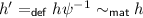
For all \(f\in {\mathsf {Hom}}(\mathcal {G})\), for all \(g,h\in {\mathsf {Hom}}(\mathcal {G})\), we say that g is extended by f into h, whenever \(g=hf\). We say that the extension is trivial when f is an iso.

An extension basis (thick arrows) describing how to “discover” \(G_1\) and \(G_2\) starting from \(G_0\). The colored A node helps tracking the identity of A through the basis: note here that the basis has two distinct ways of discovering \(G_1\) from \(G_0\), each of which has its own extension into \(G_2\). Given an initial match \(g_0\) into K, one may extend \(g_0\) into \(g_1\) through f, and then \(g_1\) into \(g_2\) through the extension h. Note that \(f'\) fails to extend \(g_0\) in K.

Two morphisms f and g that belong to the same extension class (since \(f=\phi g\)) but define two distinct matchings of G in H (there is no iso \(\psi \) such that \(f=g\psi \)).
Importantly, two maps \(g:G\rightarrow K\) and \(g':G\rightarrow K\) denoting the same match can be respectively extended by a map \(f:G\rightarrow H\) into distinct matches of H into K (Fig. 6, left diagram). Similarly, two distinct matches \(g:G\rightarrow K\) and \(g':G\rightarrow K\) might be extended by \(f:G\rightarrow H\) into maps that denote the same match (Fig. 6, right diagram).
Definition 7
(Extension step). Let \(\varGamma \subseteq {\mathsf {Hom}}(G,K)\) and \(\varGamma '\subseteq {\mathsf {Hom}}(H,K)\) for some \(G,H,K\in \mathcal {G}\). For all \(\mathcal {F}\subseteq {\mathsf {Hom}}(\mathcal {G})\), the pair \((\varGamma ,\varGamma ')\) defines an \(\mathcal {F}\)-extension step if \(\varGamma '={ Ext }_{\mathcal {F},K}(\varGamma )\) with:
For all set \(\mathcal {S}\) and \(\approx \ \subseteq \mathcal {S}\times \mathcal {S}\) an equivalence relation over elements of \(\mathcal {S}\), we define:
Definition 8
(Extension basis). Consider a set of morphisms \(\mathcal {F}\subseteq {\mathsf {Hom}}(\mathcal {G})\). We say that \(\mathcal {F}\) is an extension basis if it satisfies \([\mathcal {F}]_{{{\mathsf {ext}}}}=\{\mathcal {F}\}\).
In Definition 7, \({ Ext }_{\mathcal {F},K}(\varGamma )\) extends an arbitrary set of maps \(\varGamma \) into all possible extensions of \(g\in \varGamma \) by a map in \(\mathcal {F}\). This raises two issues: first, we wish to build extension steps between sets of matches into K and not all equivalent ways of denoting the same match. So one may wonder what one obtains if, instead of computing \({ Ext }_{\mathcal {F},K}(\varGamma )\), one were to compute \({ Ext }_{\mathcal {F},K}(\varGamma ')\) for some \(\varGamma '\in [\varGamma ]_{{{\mathsf {mat}}}}\). Second, the set \(\mathcal {F}\) might be arbitrarily large, and we wish to compute the same extension step with a smaller set of maps.

Left diagram (loosing symmetry): two equivalent matches g and \(g'\) can be extended by f into two distinct matches. Right diagram (gaining symmetry): two distinct matches g and \(g'\) can be extended by f into the same match.
The Extension theorem below provides an answer to these two issues: computing \({ Ext }_{\mathcal {F},K}(\varGamma )\) is essentially equivalent to computing \({ Ext }_{\mathcal {F}',K}(\varGamma ')\) if one picks \(\mathcal {F}'\in [\mathcal {F}]_{{{\mathsf {ext}}}}\) and \(\varGamma '\in [\varGamma ]_{{{\mathsf {mat}}}}\).
Theorem 2
(Extension). Let \(\mathcal {F}\subseteq {\mathsf {Hom}}(G,H)\), and \(\varGamma \subseteq {\mathsf {Hom}}(G,K)\). For all \(\varGamma '\in [\varGamma ]_{{{\mathsf {mat}}}}\), for all extension basis \(\mathcal {F}'\in [\mathcal {F}]_{{{\mathsf {ext}}}}\), we have:
Importantly, replacing \(\mathcal {F}\) by an arbitrary extension basis and \(\varGamma \) by an arbitrary member of \([\varGamma ]_{{{\mathsf {mat}}}}\) is not a neutral operation with respect to extension step. However the resulting set of maps is indistinguishable from \({ Ext }_{\mathcal {F},K} (\varGamma )\) if one equates matching equivalent maps.
Notice also that although \([\varGamma ']_{{{\mathsf {mat}}}}=\{\varGamma '\}\) (\(\varGamma '\) is already stripped of any redundant map), in general \([{ Ext }_{\mathcal {F}',K} (\varGamma ')]_{{{\mathsf {mat}}}}\ne \{{ Ext }_{\mathcal {F}',K} (\varGamma ')\}\) because one extension step, even using purely non equivalent extensions, may produce matching-equivalent maps (see Fig. 6, right example). However we can prove that it is not possible to extend the same map g into two matching-equivalent h and \(h'\) unless one has used extension-equivalent maps to do so:

Proof
By hypothesis we have \(hf=h'f'\). Suppose we have \(h=h'\phi \) for some iso \(\phi \). So we have \(h'\phi f=h'f'\) by substituting h in the hypothesis. Since \(h'\) is injective, we deduce \(\phi f=f'\) and  follows by Definition 5. \(\square \)
In combination with the example of Fig. 6 (right diagram), this proposition essentially guarantees that, when using an extension basis, the only way to produce matching-equivalent extensions is to start from two maps that were not matching equivalent. This remark will become handy when we describe our update algorithm in Sect. 5.
4.3 Proof of the Extension Theorem
We begin by a lemma that shows one cannot lose any match into K after the extension step if one disregards extension-equivalent maps in \(\mathcal {F}\):

Eventually we need a Lemma that shows it is also not possible to lose a match into K after the extension step, if one disregards matching-equivalent maps in \(\varGamma \).
Lemma 3
Let \(g:G\rightarrow K\), \(f:G\rightarrow H\) and \(h:H\rightarrow K\) an f-extension of g. The following proposition holds:

We are now in position to prove the Extension Theorem.
Proof
(Theorem 2). We first prove Eq. (7).
-
Suppose \({ Ext }_{\mathcal {F}',K}(\varGamma ')=\emptyset \), by definition this implies:
$$ \{h\mid \exists f\in \mathcal {F}': hf\in \varGamma '\}=\emptyset $$This can be either true because \(\varGamma '=\emptyset \) (point 1) or because no f in \(\mathcal {F}'\) satisfies \(hf\in \varGamma '\) for some h (point 2).
-
1.
Since \(\varGamma '=\emptyset \) and \(\varGamma '\in [\varGamma ]_{{{\mathsf {mat}}}}\), we have that \(\varGamma =\emptyset \). In turn, this entails that \({ Ext }_{\mathcal {F},K}(\varGamma )=\emptyset \).
-
2.
Looking for a contradiction, suppose that some \(f\in \mathcal {F}\) is such that \(hf\in \varGamma \) for some h. Since we supposed that no \(f\in \mathcal {F}'\) satisfies \(hf\in \varGamma '\) necessarily \(f\not \in \mathcal {F}'\). But since \(\mathcal {F}'\in [\mathcal {F}]_{{{\mathsf {ext}}}}\) there exists \(f'\in \mathcal {F}'\) such that
 . According to Lemma 2, there exists
  such that \(h'f'\in \varGamma '\) which entails a contradiction. Therefore no f in \(\mathcal {F}\) satisfies \(hf\in \varGamma \) for any h and \(\varGamma =\emptyset \).
-
1.
-
Suppose that \({ Ext }_{\mathcal {F},K}(\varGamma )=\emptyset \). Since \(\varGamma '\subseteq \varGamma \) it follows immediately that \({ Ext }_{\mathcal {F}',K}(\varGamma ')\subseteq { Ext }_{\mathcal {F}',K}(\varGamma ')\) and hence \({ Ext }_{\mathcal {F}',K}(\varGamma ')=\emptyset \). \(\square \)
 . According to Lemma 2, there exists
  such that
 We now prove Eq. (8). Note that it is equivalent to proving:

So let us suppose there is some h such that \(h\in { Ext }_{\mathcal {F},K}(\varGamma )\) and \(h\not \in { Ext }_{\mathcal {F}',K}(\varGamma ')\). Recall that \(h\in { Ext }_{\mathcal {F},K}(\varGamma )\) implies that \(hf\in \varGamma \) for some \(f\in \mathcal {F}\). In addition, \(h\not \in { Ext }_{\mathcal {F}',K}(\varGamma ')\) implies that for all \(f'\in \mathcal {F}'\), \(hf'\not \in \varGamma '\). Now there are several cases to consider:
-
\(f\in \mathcal {F}'\) and \(hf\in \varGamma '\). This would imply that \(h\in { Ext }_{\mathcal {F}',K}(\varGamma ')\) which would contradict our hypothesis.
-
\(f\in \mathcal {F}'\) and \(hf\not \in \varGamma '\). Since \(\varGamma '\in [\varGamma ]_{{{\mathsf {mat}}}}\) we know there exists \(g\in \varGamma '\) such that
 . We apply Lemma 3 to deduce that there exists
  and \(f'\) such that \(h'f'=g\). Still according to Lemma 3, either \(f'=f\) (point 1) or
  (point 2).
-
1.
Since \(f\in \mathcal {F}'\) we have that \(h'\in { Ext }_{\mathcal {F}',K}(\varGamma ')\).
-
2.
Since \(\mathcal {F}'\in [\mathcal {F}]_{{{\mathsf {ext}}}}\),
 implies there is
  such that \(f''\in \mathcal {F}'\). We apply Lemma 2 to deduce that there exists
  such that \(f''h''\in \varGamma '\). By transitivity of
  we have
  and we do have \(h''\in { Ext }_{\mathcal {F}',K}(\varGamma ')\).
-
1.
-
\(f\not \in \mathcal {F}'\) and \(hf\in \varGamma '\). Since \(\mathcal {F}'\in [\mathcal {F}]_{{{\mathsf {ext}}}}\) we know there exists \(f'\in \mathcal {F}'\) that satisfies
 . We apply Lemma 2 to deduce that there is
  such that \(h'f'\in \varGamma '\). It entails that \(h'\in { Ext }_{\mathcal {F}',K}(\varGamma ')\).
 -
\(f\not \in \mathcal {F}'\) and \(hf\not \in \varGamma '\) and we proceed by combining the arguments of the two previous points. \(\square \)
 . We apply Lemma
  and
and  (point 2).
 implies there is
  such that
  such that
  we have
  and we do have
  . We apply Lemma 2 to deduce that there is
  such that
 5 The Update Algorithm
In this section we show how to utilize extension bases and extension steps to implement the incremental update function specified in Sect. 3. We describe Fig. 7 the interplay of extension steps and exploration of the concrete domain.

Extension steps and domain exploration. The occurrence of \(\eta \) on K provides a map \(g:G_0\rightarrow K\) and the concrete identity of \(G_0\) in K. The algorithm looks for all possible extension steps above \(G_0\) in the statically computed basis. The extensions that succeed are represented with plain line arrows. Those that fail are represented with dotted line arrows. For instance no extension step is able to provide a match for \(G_4\) in K.
5.1 Abstract Effects
Graph rewriting systems are given as a set of rewriting rules of the form
where \({{\varvec{r}}}\) is a partial map between \(L\in \mathcal {G}\) and \(R\in \mathcal {G}\). Formally such a partial map is given as a span \({{\varvec{r}}}=\langle {{\mathsf {lhs}}:D\rightarrow L,{\mathsf {rhs}}:D\rightarrow R}\rangle \) where \(D\in \mathcal {G}\) is the domain of definition of \({{\varvec{r}}}\) and \({\mathsf {lhs}}\) (resp. \({\mathsf {rhs}}\)) stands for the left hand side map of \({{\varvec{r}}}\) (resp. right hand side). For all such span \({{\varvec{r}}}\), we define:
Definition 9
(abstract effect). Let \({{\varvec{r}}}\) be a rule. The abstract effect of \({{\varvec{r}}}\), written \({\eta }^\sharp _{{{\varvec{r}}}}\), is the pair of maps:
where \(f^\varepsilon _{{{\varvec{r}}}}\) is the identity on its domain.
We give Fig. 8 an example of the derivation of an abstract effect from a Kappa rule.

Deriving an abstract effect from a Kappa rule. The Kappa rule is given as a partial map \({{\varvec{r}}}:L\rightharpoonup R\) (upper part). The corresponding abstract effect is a pair of maps \((f_{{{\varvec{r}}}}^-,f_{{{\varvec{r}}}}^+)\) describing respectively the edges that are removed and added by the rule.
Definition 10
(K-occurrence). Consider an abstract effect
For all concrete state K, a K-occurrence \(m_{K,{{\varvec{r}}}}\) of \({\eta }^\sharp _{{{\varvec{r}}}}\) is a pair of maps:
and we write \(m_{K,{{\varvec{r}}}}({\eta }^\sharp _{{{\varvec{r}}}})=\eta \) whenever:
5.2 Extension Basis Synthesis
Recall from Sect. 2.3 that we consider a set \(\mathcal {O}\subseteq \mathcal {G}\) of observable graphs. Since the observables (including any match of the left hand sides of a rule) are intentionally given as a finite set of abstract graphs (see Sect. 2), we may assume that every elements of \([\mathcal {O}]_\mathsf {iso}\) is finite, where \(\sim _\mathsf {iso}\) is the graph isomorphism equivalence relation. Let us thus consider an arbitrary \(\hat{\mathcal {O}}\subseteq \mathcal {G}\) such that \(\hat{\mathcal {O}}\in [\mathcal {O}]_\mathsf {iso}\).
For all rule \({{\varvec{r}}}\), we define now the procedure to build a negative and positive \({{\varvec{r}}}\)-extension basis, respectively \(\mathfrak {B}_{{{\varvec{r}}}}^+\subseteq {\mathsf {Hom}}(\mathcal {G})\) and \(\mathfrak {B}_{{{\varvec{r}}}}^-\subseteq {\mathsf {Hom}}(\mathcal {G})\).
Similarly to Sect. 3 we adopt the following naming convention: for all \(r:L\rightharpoonup R\) we write \(\pi ^+_{{{\varvec{r}}}}=_{{{\mathsf {def}}}}R\) and \(\pi ^-_{{{\varvec{r}}}}=_{{{\mathsf {def}}}}L\) and the superscript \(\_^\varepsilon \) should be globally replaced by either \(\_^+\) or \(\_^-\) to specialize a definition to the positive or negative update.
Procedure 1:
“Backbone” extension basis synthesis (see Sect. 4.1 for the categorical constructions used in the procedure).
Input: a rule \({{\varvec{r}}}\) and the set of (abstract) observables \(\hat{\mathcal {O}}\).
-
1.
Compute the abstract effect \({\eta }^\sharp _{{{\varvec{r}}}}=\langle {f_{{{\varvec{r}}}}^-:H_{{{\varvec{r}}}}^-\rightarrow \pi _{{{\varvec{r}}}}^-,f_{{{\varvec{r}}}}^+:H_{{{\varvec{r}}}}^+\rightarrow \pi _{{{\varvec{r}}}}^+}\rangle \)
-
2.
For all \(O\in \hat{\mathcal {O}}\), build \(\varLambda _{O}^\varepsilon \in [{\mathsf {Gluings}}(H^\varepsilon _{{{\varvec{r}}}},O)]_{{{\mathsf {ext}}}}\)
-
3.
For all \(\langle {f:O\rightarrow G,h:H^\varepsilon _{{{\varvec{r}}}}\rightarrow G}\rangle \in \varLambda _{O}^\varepsilon \), build \(\varLambda ^\varepsilon _{O,h}\in [{\mathsf {Mpo}}(h,f_{{{\varvec{r}}}}^\varepsilon )]_{{{\mathsf {ext}}}}\)
-
4.
\(\mathfrak {B}^\varepsilon _{{{\varvec{r}}}} =_{{{\mathsf {def}}}}\{f\mid \exists O,\exists h,\exists g \hbox { s.t } \langle {g,f}\rangle \in \varLambda ^\varepsilon _{O,h}\}\)
-
5.
return \(\mathfrak {B}^\varepsilon _{{{\varvec{r}}}}\)
An important point with respect to combinatorial explosion is the following:
Proposition 6
At step 3 and for all h, \(\varLambda _{O,h}^\varepsilon \) contains at most one element.
In a nutshell, at step 2 one computes all possible gluings of \(H^\varepsilon _{{{\varvec{r}}}}\) with some observable O. At step 3 we build abstract witnesses by means of multi-pushout construction. Finally step 4 assembles into \(\mathfrak {B}^\varepsilon _{{{\varvec{r}}}}\) all extensions \(f:\pi _{{{\varvec{r}}}}^\varepsilon \rightarrow W\) that are the left component of an idem-pushout built in the previous step. We provide and example, Fig. 9, of the construction of the “backbone” extension basis in the context of Kappa.

Construction of the “backbone” extension basis \(\mathfrak {B}_{{{\varvec{r}}}}^\varepsilon = \{f_1\}\). Grey coloring of nodes helps tracking nodes of \(H_{{{\varvec{r}}}}^\varepsilon \) through the morphisms (all closed diagrams are commuting). In dotted line, the maps that are used for the construction of the basis but that are not morphisms of \(\mathfrak {B}_{{{\varvec{r}}}}^\varepsilon \). Consistently with Proposition 6, the multi-pushouts in the upper part of the diagram have at most one element (\(\varLambda _{O,h_1}^\varepsilon =\{W_1\}\), the other gluings are incompatible with \(\pi _{{{\varvec{r}}}}^\varepsilon \)).
We call this extension basis a “backbone” because it only contains direct extensions from \(\pi _{{{\varvec{r}}}}^\varepsilon \) to some witness. We will see shortly how to enrich this backbone basis into a new basis that takes into account sharing between witnesses.
In the meantime, we may readily state a lemma that guarantees that extensions steps along \(\mathfrak {B}^\varepsilon _{{{\varvec{r}}}}\) produce concrete witnesses. Consider a basis \(\mathfrak {B}_{{{\varvec{r}}}}^\varepsilon \) build from a rule \({{\varvec{r}}}\) and a set of abstract observables following Procedure 1. Recall that any K-occurrence of \({\eta }^\sharp _{{{\varvec{r}}}}\) is a pair of maps \((g_0^-,g_0^+)\) that identify the edges that are respectively removed and added in K. Whenever the \(\mathfrak {B}^\varepsilon _{{{\varvec{r}}}}\)-extension of \(\{g_0^\varepsilon \}\) (see Definition 7) builds a non empty set \(\varGamma \) of witness matches into K, then those matches indeed provide \(\eta \)-witnesses (see Sect. 3.1) that are also below \(K^\varepsilon \).
Lemma 4
(Soundness). Let \({{\varvec{r}}}\) be a rule with an abstract effect \({\eta }^\sharp _{{{\varvec{r}}}}\). Let also \(m_{K,r}=_{{{\mathsf {def}}}}(g_0^-,g_0^+)\) be a K-occurrence of \({{\varvec{r}}}\) with \(\eta =m_{K,r}({\eta }^\sharp _{{{\varvec{r}}}})\) a concrete effect. For all \((h:W\rightarrow K)\in { Ext }_{\mathfrak {B}^\varepsilon _{{{\varvec{r}}}},K^\varepsilon }(\{g_0^\varepsilon \})\), there exists \(f_K:O\rightarrow K\) such that:
A simple saturation procedure enables one to add sharing between graphs of the “backbone” extension basis we have constructed so far:
Procedure 2:
Add sharing to an extension basis.
Input: an extension basis \(\mathfrak {B}\).
-
1.
if there exists \(f,f'\in \mathfrak {B}\) and \(g,h,h'\not \in \mathfrak {B}\) such that \(f=hg\) and \(f'=h'g\) then
\(\mathfrak {B}=\mathfrak {B}\cup \{g,h,h'\}\) and go to 1.
-
2.
else return \(\mathfrak {B}\).
We write \(G<_{\mathfrak {B}}^1 H\) if there exists \(f\in \mathfrak {B}\) such that \(f:G\rightarrow H\). The relation \(\le _\mathfrak {B}\) is the transitive and reflexive closure of \(<_{\mathfrak {B}}^1\) and denotes a partial order.
5.3 Implementing the Incremental Update Function
This section is dedicated to the implementation of the incremental update function, according to the specification that was given Sect. 3.3. The algorithm relies on a pre-computation of the \({{\varvec{r}}}\)-extension bases (with sharing) of all rule \({{\varvec{r}}}\) contained in the rule set:
Procedure 3:
Compute the extension bases.
Input: a finite rule set \(\mathcal {R}\).
-
1.
For all \(r\in \mathcal {R}\), build \(\mathfrak {B}_{{{\varvec{r}}}}^\varepsilon \) following Procedure 1.
-
2.
For all \(\mathfrak {B}_{{{\varvec{r}}}}^\varepsilon \), add sharing following Procedure 2.
-
3.
return \(\bigcup _{{{\varvec{r}}}} \{\mathfrak {B}_{{{\varvec{r}}}}^\varepsilon \}\).
Each time a rule \({{\varvec{r}}}\) is applied to a graph K, one obtains the corresponding K-occurrence \(m_{K,{{\varvec{r}}}}=(g_0^+:\pi _{{{\varvec{r}}}}^+\rightarrow K,g_0^+:\pi _{{{\varvec{r}}}}^+\rightarrow K)\). We use \(g_0^\varepsilon \) as an input to the update procedure, which is a breadth-first traversal of the extension basis \(\mathfrak {B}_{{{\varvec{r}}}}^\varepsilon \):
Procedure 4:
Incremental update.
Input: a basis \(\mathfrak {B}_{{{\varvec{r}}}}^\varepsilon \), a K-occurrence \(g_0^\varepsilon :\pi _{{{\varvec{r}}}}^\varepsilon \rightarrow K\) of \({\eta }^\sharp _{{{\varvec{r}}}}\), and a predicate \(w:\mathcal {G}\rightarrow 2\) such that w(G) holds if G is an abstract witness of \(\mathfrak {B}_{{{\varvec{r}}}}^\varepsilon \). For all set of morphisms \(\mathcal {F}\subseteq \mathfrak {B}_{{{\varvec{r}}}}^\varepsilon \) we define:
-
1.
Initialize \(\gamma :\mathcal {G}\rightarrow \mathcal {P}({\mathsf {Hom}}(\mathcal {G}))\) as \(\gamma (G):=\emptyset \) for all \(G\ne \pi _{{{\varvec{r}}}}^\varepsilon \) and \(\gamma (\pi _{{{\varvec{r}}}}^\varepsilon ):=\{g_0\}\)
-
2.
\(\mathcal {F}:=\emptyset \) (for the extensions yet to explore), \(x:=\pi _{{{\varvec{r}}}}^\varepsilon \) (for the current point in the basis) and \(\mathcal {W}:=\emptyset \) (for the reached witnesses).
-
3.
if w(x) then \(\mathcal {W} := \mathcal {W}\cup \{x\}\)
-
4.
for all \((f:x\rightarrow G)\in \mathfrak {B}_{{{\varvec{r}}}}^\varepsilon \) do \(\mathcal {F} := \mathcal {F}\cup \{f\}\)
-
5.
if \(\mathcal {F}\ne \emptyset \) then
-
6.
choose \((f:G\rightarrow H)\in \min (\mathcal {F})\)
-
7.
\(\gamma (H):= [\gamma (H)\cup { Ext }_{\{f\},K^\varepsilon }(\gamma (G))]_{{{\mathsf {mat}}}}\)
-
8.
\(\mathcal {F}:=\mathcal {F}\backslash \{f\}\) and \(x:=H\)
-
9.
go to step 3.
-
10.
else return \(\mathcal {W}_{\eta ,K}^\varepsilon \) where:
$$ \mathcal {W}_{\eta ,K}^\varepsilon := \bigcup \{W\mid \exists G\in \mathcal {W},\exists g\in \gamma (G): g(G)=W\}. $$
The procedure builds the function \(\gamma \) that maps the graphs of the basis to the matches they have in K. Initially only \(\pi _{{{\varvec{r}}}}^\varepsilon \) has a match given by \(g_0^\varepsilon \) and \(\gamma \) is updated at step 7 each time an extension step is performed. We give Fig. 10 an example of the construction of the map \(\gamma \) for a specific extension basis.

An extension basis (left) for the observables \(O_1\) (line), \(O_2\) (square), \(O_3\) (triangle) and \(O_4\) (house) and \(\pi _{{{\varvec{r}}}}^\varepsilon =H^\varepsilon =G_0\) (creation or deletion of a single edge). A concrete graph state \(K^\varepsilon \) (middle) and a representation of the final \(\gamma \) map (right). The concretization is performed using the initial match \(G_0\mapsto \{u,z\}\) (the edge \(\{u,z\}\) of \(K^\varepsilon \) has been created or deleted by the effect occurrence). Colored nodes help tracking the identity of the nodes of \(G_0\) (all closed diagrams are commuting). Overall 5 new instances of \(O_1\) were found, 1 instance of \(O_2\), 2 instances of \(O_3\) and 3 instances of \(O_4\).
We conclude this section by proving that the above procedure complies with the specification of the incremental update function given Sect. 3.3.
5.4 Correctness Proof
We essentially need to follow the guidelines of Sect. 3.3. Let:
and
We write \(\mathsf {inc}^{\varepsilon }_{\eta ,K}(X_0,\mathcal {R}_0)=(X_1,\mathcal {R}_1)\) if at step 3 we have \(X(\gamma )=X_0\) and \(\mathcal {R}(\gamma ,\mathcal {W})=\mathcal {R}_0\) and the next values of \(X(\gamma )\) and \(\mathcal {R}(\gamma ,\mathcal {W})\) are respectively \(X_1\) and \(\mathcal {R}_1\).
We begin by proving that \(\mathsf {inc}^{\varepsilon }_{\eta ,K}(X_0,\mathcal {R}_0)=(X_1,\mathcal {R}_1)\) satisfies the requirements for \(X_i\). After one loop of the procedure we have two cases:
-
if Step 5 was satisfied, then at step 7, \(X_1=X_0\cup X\) where:
$$ X=\bigcup \{G'\subseteq K^\varepsilon \mid \exists g\in \gamma (H): G' = g(H)\} $$by construction \(X\subseteq K^\varepsilon \) and \(X\cap X_0\ne \emptyset \) since a new extension step has been performed. Furthermore \(X\in \mathcal {D}^{\varepsilon }(\eta )\) by construction of the basis: it is either itself an abstract witness or it is below some other witnesses. Therefore we satisfy Eq. (5) (Sect. 3.3).
-
if Step 10 was satisfied then \(X_0=X_1\) since \(\gamma \) is not modified.
We need to prove now that \(\mathsf {inc}^{\varepsilon }_{\eta ,K}(X_0,\mathcal {R}_0)=(X_1,\mathcal {R}_1)\) satisfies the requirements for \(\mathcal {R}_i\). The only step where \(\mathcal {W}\) is modified is at step 3. Using Lemma 4 we know that for all \(G\in \mathcal {W}\), we have:
for some concrete observable \(O\subseteq K^\varepsilon \). Thus we have either \(\mathcal {R}_0=\mathcal {R}_1\) or:
and therefore the Eq. (6) is also satisfied. \(\square \)
6 Conclusion
We have investigated in this paper the problem of efficiently updating observable counts in a graph after a rewrite step has occurred. We believe our approach has several merits.

A comparison between the average time of KaSim 3 runs (in red) vs. KaSim 4 runs (in blue) on successive variants of the “ring assembly” model. KaSim 4. Scales linearly with the maximal size of the largest observable (the left hand side of the largest rule), while KaSim 3. Scales with the total number of rules in each model. (Color figure online)
The first one is of methodological nature: to our knowledge it is the first attempt to describe a problem that is usually treated in a purely algorithmic fashion [14], using domain theoretic arguments for proofs and categorical constructions for the implementation. In particular algorithmic approaches tend to consider quite concrete graphs, represented by their adjacency matrices, while graph rewriting literature uses morphisms to track node identity. We have seen here that it is possible to conciliate both worlds through the interplay between extension maps and matchings.
The second merit is of qualitative nature. The incremental update procedure that is described in this paper has been implemented in the version 4.x of KaSim, a stochastic simulator for the rewriting of Kappa models. We show Fig. 11 a comparison between runs of KaSim 3 vs. 4. On variations of the “ring assembly model” that is designed to highlight the benefits of sub-graph sharing: the number of rules each variants of the model has, grows exponentially with the size of their largest left hand side: each variant of the model is characterized by the length of a ring-like graph it is trying to form. The first variant is forming all rings up-to length 10, while the last variant is forming all rings up-to length 36. Forming all possible rings up-to length n requires !n rules, and the largest left hand side of these rules has length n.
As usual there are multiple continuations of this work one may envision. Just to mention a promising one, it would be interesting to see what happens if instead of incrementally maintaining \(\mathcal {O}_K\) (the observable that are present in state K) one were to maintain \(\mathop {\downarrow \!\!\mathcal {O}_K}\). In theory one could benefit from having partial observables already explored in order to minimize what remains to be discovered after an effect has occurred. From an implementation point of view this may lead to potentially memory intensive data structures but to very minimalist update phases.
Notes
- 1.
More than 18,000 papers mentioning the protein EGFR, a major signaling protein, either in their title or abstract have been published since 2012. For the year 2015 only there are nearly 5,000 papers for EGFR (source pubmed).
- 2.
To fix the intuition, let us say that a realistic model of cell signaling would have a few million agents of about a hundred protein types, and several hundreds of rewrite rules, possibly thousands when refinements are automatically generated.
- 3.
All rewriting techniques satisfy these properties, although only double pushout guarantees the absence of side effect.
References
Rowland, M.A., Deeds, E.J.: Crosstalk and the evolution of specificity in two-component signaling. PNAS 111(25), 9325 (2014)
Danos, V., Feret, J., Fontana, W., Harmer, R., Krivine, J.: Rule-based modelling of cellular signalling. In: Caires, L., Vasconcelos, V.T. (eds.) CONCUR 2007. LNCS, vol. 4703, pp. 17–41. Springer, Heidelberg (2007). doi:10.1007/978-3-540-74407-8_3
Faeder, J.R., Blinov, M.L., Hlavacek, W.S.: Rule-based modeling of biochemical systems with bionetgen. Methods Mol. Biol. 500, 113–167 (2009)
Danos, V., Feret, J., Fontana, W., Krivine, J.: Scalable simulation of cellular signaling networks. In: Shao, Z. (ed.) APLAS 2007. LNCS, vol. 4807, pp. 139–157. Springer, Heidelberg (2007). doi:10.1007/978-3-540-76637-7_10
Boutillier, P., Feret, J., Krivine, J. (2008). https://github.com/kappa-dev/kasim
Sneddon, M.W., Faeder, J.R., Emonet, T.: Efficient modeling, simulation and coarse-graining of biological complexity with NFsim. Nat. Methods 8, 177–183 (2011)
Danos, V., Heckel, R., Sobocinski, P.: Transformation and refinement of rigid structures. In: Giese, H., König, B. (eds.) ICGT 2014. LNCS, vol. 8571, pp. 146–160. Springer, Heidelberg (2014). doi:10.1007/978-3-319-09108-2_10
Girard, J.-Y.: The system F of variable types fifteen years after. Theor. Comput. Sci. 45, 159–192 (1986)
Ehrig, H., Pfender, M., Schneider, H.J.: Graph grammars: an algebraic approach. In: Proceedings of IEEE Conference on Automata and Switching Theory, pp. 167–180 (1973)
Raoult, J.C.: On graph rewriting. TCS 32, 1–24 (1984)
Corradini, A., Heindel, T., Hermann, F., König, B.: Sesqui-pushout rewriting. In: Corradini, A., Ehrig, H., Montanari, U., Ribeiro, L., Rozenberg, G. (eds.) Proceedings of ICGT 2006, pp. 30–45 (2006)
Milner, R.: The Space and Motion of Communicating Agents. Cambridge University Press, Cambridge (2009)
Feret, J., Danos, V., Fontana, W., Harmer, R., Krivine, J.: Internal coarse-graining of molecular systems. PNAS 106, 6453–6458 (2009)
Varró, G., Varró, D.: Graph transformation with incremental updates. ENTCS 109, 71–83 (2004). Proceedings of the Workshop on Graph Transformation and Visual Modelling Techniques (GT-VMT 2004)
Acknowledgments
This work was supported by the ANR grant ICEBERG (ANR-10-BINF-0006) and is partially sponsored by the Defense Advanced Research Projects Agency (DARPA) and the U.S. Army Research Office under grant number W911NF-14-1-0367. The views, opinions, and/or findings contained in this paper are those of the authors and should not be interpreted as representing the official views or policies, either expressed or implied, of the Defense Advanced Research Projects Agency or the Department of Defense.
Author information
Authors and Affiliations
Corresponding author
Editor information
Editors and Affiliations
Appendix
Appendix
Proofs Omitted in Section 3
Proof
(Proposition 1). We first prove Eq. (2), \(\Rightarrow \). By unfolding the def. of \(W\rhd _{\eta }^{-} O\) and by \(W\subseteq K\) we have \(O\cup {\mathsf {pre}}(\eta )\subseteq K\). As a consequence, \(O\subseteq K\) and by def. of \({{\mathsf {Obs}}}\) (Sect. 3) we have \(O\in ({{\mathsf {Obs}}}\ K)\). Still by definition of \(W\rhd _{\eta }^{-} O\) we have \(O\cap H_\eta ^-\ne \emptyset \) (i). By def. of \(\eta \mathop {\cdot }K\) (Sect. 2.2) we have \(O\backslash H_\eta ^-\cup H_\eta ^+\subseteq \eta \mathop {\cdot }K\) (ii). In addition \(H_\eta ^-\cap H_\eta ^+=\emptyset \). By (i) and (ii) we have \(O\not \subseteq \eta \mathop {\cdot }K\) and consequently \(O\not \in ({{\mathsf {Obs}}}\ \eta \mathop {\cdot }K)\).
We now prove Eq. (2), \(\Leftarrow \). By def. \(W=O\cup {\mathsf {pre}}(\eta )\) (i), and by hyp. we have \(O\in ({{\mathsf {Obs}}}\ K)\) implies \(O\subseteq K\) (ii). Moreover since \(\eta \mathop {\cdot }K\) is defined we have \({\mathsf {pre}}(\eta )\subseteq K\) (iii). From (i)–(iii) we get \(O\cup {\mathsf {pre}}(\eta )\subseteq K\). In order to conclude that \(W=O\cup {\mathsf {pre}}(\eta )\in \mathcal {W}_\eta ^-\) we need to additionally show that \(O\cap H_\eta ^-\ne \emptyset \). Since \(O\not \in ({{\mathsf {Obs}}}\ \eta \mathop {\cdot }K)\) and \(O\in ({{\mathsf {Obs}}}\ K)\) we have \(O\not \subseteq (O\backslash H_\eta ^-\cup H^+_\eta )\) (iv). Since \(H_\eta ^-\cap H_\eta ^+=\emptyset \) by def. of \(\eta \), the only possibility to satisfy (iv) is \(O\cap H_\eta ^-\ne \emptyset \). \(\square \)
Proofs Omitted in Section 4
Proof
(Lemma 2). It suffices to take \(h''=h'\phi \) which, by Definition 6 implies that  . By hypothesis we have \(g=h'f'\) and \(f'=\phi f\). From these equalities we get \(g=h'\phi f\). By substituting \(h'\phi \) by \(h''\) we obtain \(g=h'' f\). \(\square \)
Proofs Omitted in Section 5
Proof
(Lemma 3). By hypothesis we start from the following commuting diagram:
Since  , by Definition 6, we have \(g=g'\phi \) for some iso \(\phi \). We have two cases:

-
either f is \(\phi \)-preserving and there exists an iso \(\psi \) such that \(f\phi =\psi f\). Then by construction \(h\psi ^{-1}f=g'\) and we can conclude by noticing that
 (by Definition 6).
 -
or f is not \(\phi \)-preserving and there is no iso \(\psi \) such that \(f\phi =\psi f\). It entails that
 (by Definition 5) and (by symmetry)
 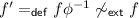 . Now we can conclude, since by construction \(hf'=g'\). \(\square \)
 (by Definition 6).
 (by Definition 5) and (by symmetry)
  . Now we can conclude, since by construction
 Proof
(Proposition 6). We have the following diagram:

where \({\varvec{h}}=\langle {h',h}\rangle \) is a gluing of O and \(H_r^\varepsilon \). Now the procedure attempts to build the multi-pushout of the span \({\varvec{f}}=\langle {h,f_r^\varepsilon }\rangle \). Suppose it has at least two elements, we have the following diagram:

where \(\langle {ih',kf_r^\varepsilon }\rangle \) and \(\langle {jh',lf_r^\varepsilon }\rangle \) are bounds for \({\varvec{h}}=\langle {h,h'}\rangle \). By construction \({\varvec{h}}\) is a relative pushout, therefore, by Proposition 4, there exists an iso \(\phi :U\rightarrow U'\) that equates the bounds \(\langle {i,k}\rangle \) and \(\langle {j,l}\rangle \). This would entail  which contradicts the hypothesis. \(\square \)
Proof
(Lemma 4). Recall from Sect. 3.1 that a (concrete) \(\eta \)-witness W for a (concrete) observable O must satisfy:
By construction of the basis, and using the hypothesis of the lemma we have the following diagram:

We take \(f_K=_{{{\mathsf {def}}}}hf_2f_1\), \(g^\varepsilon =g_0^\varepsilon f_r^\varepsilon \), and we have:
and
which verifies Eq. (10). \(\square \)
Rights and permissions
Copyright information
© 2017 Springer-Verlag GmbH Germany
About this paper
Cite this paper
Boutillier, P., Ehrhard, T., Krivine, J. (2017). Incremental Update for Graph Rewriting. In: Yang, H. (eds) Programming Languages and Systems. ESOP 2017. Lecture Notes in Computer Science(), vol 10201. Springer, Berlin, Heidelberg. https://doi.org/10.1007/978-3-662-54434-1_8
Download citation
DOI: https://doi.org/10.1007/978-3-662-54434-1_8
Published:
Publisher Name: Springer, Berlin, Heidelberg
Print ISBN: 978-3-662-54433-4
Online ISBN: 978-3-662-54434-1
eBook Packages: Computer ScienceComputer Science (R0)
