Consolidating Inner Product Masking

Abstract

Masking schemes are a prominent countermeasure to defeat power analysis attacks. One of their core ingredients is the encoding function. Due to its simplicity and comparably low complexity overheads, many masking schemes are based on a Boolean encoding. Yet, several recent works have proposed masking schemes that are based on alternative encoding functions. One such example is the inner product masking scheme that has been brought towards practice by recent research. In this work, we improve the practicality of the inner product masking scheme on multiple frontiers. On the conceptual level, we propose new algorithms that are significantly more efficient and have reduced randomness requirements, but remain secure in the t-probing model of Ishai, Sahai and Wagner (CRYPTO 2003). On the practical level, we provide new implementation results. By exploiting several engineering tricks and combining them with our more efficient algorithms, we are able to reduce execution time by nearly 60% compared to earlier works. We complete our study by providing novel insights into the strength of the inner product masking using both the information theoretic evaluation framework of Standaert, Malkin and Yung (EUROCRYPT 2009) and experimental analyses with an ARM microcontroller.

These keywords were added by machine and not by the authors. This process is experimental and the keywords may be updated as the learning algorithm improves.

1 Introduction

Physical side-channel attacks where the adversary exploits, e.g., the power consumption [34] or the running time [33] of a cryptographic device are one of the most powerful cyberattacks. Researchers have shown that they can extract secret keys from small embedded devices such as smart cards [22, 34], and recent reports illustrate that also larger devices such as smart phones and computers can be attacked [4, 24]. Given the great threat potential of side-channel attacks there has naturally been a large body of work proposing countermeasures to defeat them [35]. One of the most well-studied countermeasures against side-channel attacks – and in particular, against power analysis – are masking schemes [12, 29]. The basic idea of a masking scheme is simple. Since side-channel attacks attempt to learn information about the intermediate values that are produced by a cryptographic algorithm during its evaluation, a masking scheme conceals these values by hiding them with randomness.

Masking schemes have two important ingredients: a randomized encoding function and a method to securely compute with these encodings without revealing sensitive information. The most common masking scheme is Boolean masking [12, 32], which uses a very simple additive n-out-of-n secret sharing as its encoding function. More concretely, to encode a bit b we sample uniformly at random bits $(b_1, \ldots , b_n)$ such that $\sum _i b_i = b$ (where the sum is in the binary field). The basic security property that is guaranteed by the encoding function is that if the adversary only learns up to $n-1$ of the shares then nothing is revealed about the secret b. The main challenge in developing secure masking schemes has been in lifting the security properties guaranteed by the encoding function to the level of the entire masked computation. To this end, we usually define masked operations for field addition and field multiplication, and show ways to compose them securely.

The most standard security property that we want from a masking scheme is to resist t-probing attacks. To analyze whether a masking scheme is secure against t-probing attacks we can carry out a security analysis in the so-called t-probing model – introduced in the seminal work of Ishai et al. [32]. In the t-probing model the adversary is allowed to learn up to t intermediate values of the computation, which shall not reveal anything about the sensitive information, and in particular nothing about the secret key used by a masked cryptographic algorithm. In the last years, there has been a flourishing literature surrounding the topic of designing better masking schemes, including many exciting works on efficiency improvements [11, 14, 16, 37, 42], stronger security guarantees [18, 21, 39, 41] and even fully automated verification of masking schemes [5, 6] – to just name a few.

As mentioned previously, the core ingredient of any masking scheme is its encoding function. We can only hope to design secure masking schemes if we start with a strong encoding function at first place. Hence, it is natural to ask what security guarantees can be offered by our encoding functions and to what extent these security properties can be lifted to the level of the masked computation. Besides the Boolean masking which is secure in the t-probing model, several other encoding functions which can be used for masking schemes have been introduced in the past. This includes the affine masking [23], the polynomial masking [28, 40] and the inner product masking [1, 2, 20]. Each of these masking functions offers different trade-offs in terms of efficiency and what security guarantees it can offer.

The goal of this work, is to provide novel insights into the inner product masking scheme originally introduced by Dziembowski and Faust [20] and Goldwasser and Rothblum [25], and later studied in practice by Balasch et al. [1, 2]. Our main contribution is to consolidate the work on inner product masking thereby improving the existing works of Balasch et al. [1, 2] on multiple frontiers and providing several novel insights. Our contributions can be summarized as follows.

New algorithms with $t\textendash \mathsf {SNI}$ security property. On a conceptual level we propose simplified algorithms for the multiplication operation protected with inner product masking. In contrast to the schemes from [1, 2] they are resembling the schemes originally proposed by Ishai et al. [32] (and hence more efficient and easier to implement than the schemes in [1]), but work with the inner product encoding function. We prove that our new algorithms satisfy the property of t-strong non-interference ($t\textendash \mathsf {SNI}$) introduced by Barthe et al. [5, 6], and hence can safely be used for larger composed computation. An additional contribution is that we provide a new secure multiplication algorithm – we call it $\mathtt {IPMult}^{(2)}_{{\varvec{L}}}$ shown in Algorithm 7 – that can result in better efficiency when composed with certain other masked operations. Concretely, when we want to compose a linear function g() with a multiplication, then either we can use $\mathtt {IPMult}^{(1)}_{{\varvec{L}}}$ and require an additional refreshing operation at the output of g(), or we use our new algorithm $\mathtt {IPMult}^{(2)}_{{\varvec{L}}}$ that eliminates the need for the additional refreshing. This can save at least $\mathcal {O}(n^2)$ in randomness.

New implementation results. We leverage on the proposed algorithms for the multiplication operation to build new software implementations of AES-128 for embedded AVR architectures. Compared to earlier works [1], we are able to reduce the execution times by nearly a factor 60% (for 2 shares) and 55% (for 3 shares). The improvements stem not only from a decrease in complexity of the new algorithms, but also from an observation that enables the tabulation of the AES affine transformation. We additionally provide various flavors of AES-128 implementations protected with Boolean masking, using different addition chains that have been proposed to compute the field inversion. Our performance evaluation allow us to quantify the current gap between Boolean and IP masking schemes in terms of execution time as well as non-volatile storage.

Information theoretic evaluation. We continue our investigations with a comprehensive information theoretic evaluation of the inner product encoding. Compared to the previous works of Balasch et al., we consider the mutual information between a sensitive variable and the leakage of its inner product shares for an extended range of noises, for linear and non-linear leakage functions and for different values of the public vector of the encoding. Thanks to these evaluations, we refine the understanding of the theoretical pros and cons of such masking schemes compared to the mainstream Boolean masking. In particular, we put forward interesting properties of inner product masking regarding “security order amplification” in the spirit of [9, 10, 31] and security against transition-based leakages [3, 15]. We also highlight that these interesting properties are quite highly implementation-dependent.

Experimental evaluation. Eventually, we confront our new algorithms and their theoretical analyses with practice. In particular, we apply leakage detection techniques on measurements collected from protected AES-128 routines running on an ARM Cortex-M4 processor. Our results reveal the unequivocal presence of leakage (univariate, first-order) in the first-order Boolean masked implementation. In contrast the first-order inner product masked implementation shows significantly less evidence of leakage (with the same number of measurements). Combined with the previous proofs and performance evaluations, these results therefore establish inner product masking as an interesting alternative to Boolean masking, with good properties for composability, slight performance overheads and significantly less evidence of leakage.

2 Notation

In the following we denote by $\mathcal {K}$ a field of characteristic 2. We denote with upper-case letters the elements of the field $\mathcal {K}$ and with bold notation that one in the $\mathcal {K}$-vector spaces. The field multiplication is represented by the dot $\cdot$ while the standard inner product over $\mathcal {K}$ is denoted as $\langle \varvec{X}, \varvec{Y} \rangle =\sum _iX_i \cdot Y_i$, where $X_i$ and $Y_i$ are the components of the vectors $\varvec{X}$ and $\varvec{Y}$.

The symbol $\delta _{ij}$ corresponds to the element 0 when $i=j$ and 1 otherwise.

3 New Algorithm

Our new multiplication scheme is based on the inner product construction of Dziembowski and Faust [20] and constitutes an improvement to the works [1, 2]. The encoding of a variable $S \in \mathcal {K}$ consists of a vector $\varvec{S} \in \mathcal {K}^n$ such that $S=\langle {\varvec{L}}, \varvec{S} \rangle$, where ${\varvec{L}}$ is a freely chosen, public non-zero parameter with first component $L_1=1$.

The algorithms for initialization and masking are depicted in the $\mathtt {IPSetup}$ and $\mathtt {IPMask}$ procedures. The subroutine $\mathtt {rand}(\mathcal {K})$ samples an element uniformly at random from the field $\mathcal {K}$.

The algorithms for addition and refreshing are kept the same as in [1], while a new multiplication scheme $\mathtt {IPMult}^{(1)}$ is proposed in Algorithm 3. The schemes achieves security order $t=n-1$ in the t-probing model.

Our starting point for the Algorithm 3 is the multiplication scheme from [32]. We reuse the idea of summing the matrix of the inner products of the inputs with a symmetric matrix of random elements, in order to compute the shares of the output in a secure way. In particular we design these two matrices ($\varvec{T}$ and $\varvec{U}'$ in the algorithm) to be consistent with our different masking model.

The correctness of the scheme is proved in the following lemma.

Lemma 1

For any ${\varvec{L}},\varvec{A},\varvec{B}\in \mathcal {K}^n$ and $\varvec{C}= \mathtt {IPMult}^{(1)}_{\varvec{L}}(\varvec{A},\varvec{B})$, we have

$$\langle {\varvec{L}}, \varvec{C} \rangle = \langle {\varvec{L}}, \varvec{A} \rangle \cdot \langle {\varvec{L}}, \varvec{B} \rangle .$$

Proof

For all $i\ne j$ it holds:

$$\begin{aligned} \langle {\varvec{L}}, \varvec{C} \rangle&= \sum _i L_i \cdot C_i = \sum _i L_i\sum _j V_{i,j}=\sum _iL_i\sum _j(T_{ij}+U_{ij}) \\ {}&=\sum _iL_i\sum _j(A_iB_jL_j+U'_{ij}L_i^{-1})=\sum _iL_i\sum _jA_iB_jL_j+\sum _{ij}U'_{ij}\\&=\sum _iL_iA_i\sum _jB_jL_j=\langle {\varvec{L}}, \varvec{A} \rangle \langle {\varvec{L}}, \varvec{B} \rangle \end{aligned}$$

   $\square$

3.1 Security Proof

We analyze the security of our new multiplication scheme in the t-probing model, introduced in the seminal work of Ishai et al. [32], in which the adversary is allowed to learn up to t intermediate values that are produced during the computation. In particular we prove our algorithm to be secure also when composed with other gadgets in more complex circuits, by proving the stronger property of $t-$ Strong Non-Interference ($t\textendash \mathsf {SNI}$) defined by Barthe et al. in [5] and recalled in the following.

Definition 1

( $t-$ Strong Non-Interferent). An algorithm $\mathcal {A}$ is $t-$ Strong Non-Interferent ($t\textendash \mathsf {SNI}$) if and only if for any set of $t_1$ probes on intermediate variables and every set of $t_2$ probes on output shares such that $t_1+t_2\le t$, the totality of the probes can be simulated by only $t_1$ shares of each input.

In a few words the property requires not only that an adversary can simulate $d< t$ probes with d inputs, like in the classical t-probing model, but also that the number of input shares needed in the simulation are independent from the number of probes on the output shares.

The following lemma shows the $t\textendash \mathsf {SNI}$ security of $\mathtt {IPMult}_{{\varvec{L}}}^{(1)}$.

Lemma 2

The algorithm $\mathtt {IPMult}_{{\varvec{L}}}^{(1)}$ is $t\textendash \mathsf {SNI}$ with $t=n-1$.

Proof

Let $\varOmega =(\mathcal {I},\mathcal {O})$ be a set of t observations respectively on the internal and on the output wires, where $|\mathcal {I}|=t_1$ and in particular $t_1+|\mathcal {O}|\le t$. We construct a perfect simulator of the adversary’s probes, which makes use of at most $t_1$ shares of the secrets $\varvec{A}$ and $\varvec{B}$.

Let $w_1, \dots , w_t$ be the probed wires. We classify the internal wires in the following groups:

• (1) $A_i,B_i$,

• (2) $U_{i,j}, U'_{i,j}$,

• (3) $A_i\cdot B_j, T_{i,j}, V_{i,j}$,

• (4) $C_{i,j}$, which represents the value of $C_i$ at iteration i, j of the last for loop.

We define two sets of indices I and J such that $|I|\le t_1$, $|J|\le t_1$ and the values of the wires $w_h$ with $h=1,\dots , t$ can be perfectly simulated given only the knowledge of $(A_i)_{i \in I} \text { and } (B_i)_{i \in J}$. The sets are constructed as follows.

• Initially I and J are empty.

• For every wire as in the groups (1), (2) and (4), add $i \text { to } I$ and to J.

• For every wire as in the group (3) if $i\notin I$ add $i \text { to } I$ and if $j \notin J$ add $j \text { to } J$.

Since the adversary is allowed to make at most $t_1$ internal probes, we have $|I|\le t_1$ and $|J|\le t_1$.

We now show how the simulator behaves, by starting to consider the internal observed wires.

• 1. For each observation as in the group (1), by definition of I and J the simulator has access to $A_i,B_i$ and then the values are perfectly simulated.

• 2. For each observation as in the group (2), we distinguish two possible cases:

  • If $i\in I,J$ and $j\notin J$, the simulator assigns a random and independent value to $U'_{i,j}$: if $i<j$ this is what would happen in the real algorithm, otherwise since $j \notin J$ the element $U'_{ij}$ will never enter into the computation of any $w_h$ (otherwise j would be in J).

  • If $i\in I,J$ and $j\in J$, the values $U'_{i,j}$ and $U'_{j,i}$ can be computed as in the actual circuit: one of them (say $U'_{j,i}$) is assigned to a random and independent value and the other $U'_{i,j}$ to $-U'_{i,j}$.

  The value $U_{i,j}$ is computed using the simulated $U'_{i,j}$ and the public value $L_i$.

• 3. For each observation as in the group (3), by definition of the sets I and J and for the previous points, the simulator has access to $A_i, A_j, B_i, B_j$, to the public value $L_j$ and $U_{i,j}, U'_{i,j}$ can be simulated. Therefore $A_i \cdot B_j, T_{i,j}$ and $V_{i,j}$ can be computed as in the real algorithm.

• 4. For each observation as in the group (4), by definition $i\in I,J$. At first we assign a random value to every summand $V_{ik}$, with $k\le j$ and $k\notin J$, entering in the computation of any observed $C_{ij}$. Then if one of the addends $V_{ik}$ with $k\le j$ composing $C_{ij}$ has been probed, since by definition $k\in J$, we can simulate it as in Step 3. Otherwise $V_{ik}$ has been previously assigned at the beginning of the current Step 4.

We now simulate the output wires $C_i$. We have to take into account the following cases.

• 1. If the attacker has already observed some intermediate values of the output share $C_i$, we note that each $C_i$ depends on the random values in the i ^th row of the matrix $\varvec{U'}$, i.e. $U'_{il}$ for $l<i$ and $U'_{li}$ for $l>i$. In particular each of the $U'_{il}$ appears a second time in one of the remaining $C_1, \cdots , C_{i-1}, C_{i+1}, \cdots , C_n$, as shown in the following matrix.

  

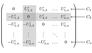
  Since each $C_i$ depends on $n-1$ random values and the adversary may have probed at most $n-2$ of that, then independently of the intermediate elements probed, at least one of the $U'_{il}$ doesn’t enter into the computation of $C_{i,j}$ and so $C_i$ can be simulated as a random value.

• 2. If all the partial sums have been observed, we can use the values previously simulated and add them according to the algorithm. Finally it remains to simulate a $C_i$ when no partial sum $C_{ij}$ has been observed. By definition, at least one of the $U'_{il}$ involved in the computation of $C_i$ is not used in any other observed wire. Therefore we can assign a random value to $C_i$.

   $\square$

4 Application to AES Sbox

Since $\mathtt {IPMult}^{(1)}_{{\varvec{L}}}$ is proved to be $t\textendash \mathsf {SNI}$, it can be securely composed with other $t\textendash \mathsf {SNI}$ or affine gadgets. In the following we analyze more in detail the algorithm for the exponentiation to the power 254 in $\mathrm {GF}(2^8)$, which constitutes the non-linear part of the AES Sbox. We consider Rivain and Prouff’s algorithm from [17, 42]. We recall the squaring routine $\mathtt {IPSquare}_{{\varvec{L}}}$ and the refreshing scheme from [1]. We give in particular a $t\textendash \mathsf {SNI}$ refreshing $\mathtt {SecIPRefresh}_{{\varvec{L}}}$, which essentially consists in the execution of $\mathtt {IPRefresh}_{{\varvec{L}}}$ n times. In [1] the authors already remarked that such a scheme ensures security even if composed with other gadgets, but no formal proof was provided. In the following we formally analyze the security of the algorithm, by giving the proof of $t\textendash \mathsf {SNI}$.

Lemma 3

The algorithm $\mathtt {SecIPRefresh}_{{\varvec{L}}}$ is $t\textendash \mathsf {SNI}$ with $t=n-1$.

Proof

Let $\varOmega =(\mathcal {I},\mathcal {O})$ be a set of t observations respectively on the internal and on the output wires, where $|\mathcal {I}|=t_1$ and in particular $t_1+|\mathcal {O}|\le t$. We point out the existence of a perfect simulator of the adversary’s probes, which makes use of at most $t_1$ shares of the secret $\varvec{X}$.

The internal wires $w_h$ are classified as follows:

• (1) $X_i$

• (2) $A_{i,j}$, which is the component i of the vector $\varvec{A}$ in the j ^th $\mathtt {IPRefresh}_{{\varvec{L}}}$

• (3) $Y_{i,j}=X_i+\sum _{k=1}^{j}A_{i,k}$, which is the component i of $\varvec{Y}$ in the j ^th $\mathtt {IPRefresh}_{{\varvec{L}}}$

We define a set of indices I such that $|I|\le t_1$ as follows: for every observation as in the group (1), (2) or (3) add i to I.

Now we construct a simulator that makes use only of $(X_i)_{i\in I}$.

• For each observation as in the group (1), $i\in I$ and then by definition of I the simulator has access to the value of $X_i$.

• For each observation as in the group (2), $A_{i,j}$ can be sample uniformly at random. Indeed, this is what happens in the real execution of the algorithm for the shares $A_{i,j}$ with $i=2, \dots , n$. Otherwise, since we have at most $n-1$ probes, the adversary’s view of $A_{1,j}$ is also uniformly random.

• For each observation as in the group (3), $X_i$ can be perfectly simulated, $A_{i,j}$ can be sampled as in the real execution of the algorithm, and then all the partial sums $Y_{i,j}$ can be computed.

As for the output wires, we distinguish two cases. If some partial sum has already been observed, we remark that each output share $Y_{i,n}$ involves the computation of $n-1$ random bits $A_{i,1}, \dots , A_{i,n-1}$. The situation can be better understood from the following matrix, which shows the use of the random bits for each output share.

Now, since the adversary can have just other $n-2$ observations, there exists at least one non-observed random bit and we can simulate $Y_{i,n}$ as a uniform and independent random value. Moreover, if all the partial sums have been observed, we can use the values previously simulated and add them according to the algorithm. Otherwise, if no partial sum has been probed, since the random values involved in the computation of $Y_{1,n}, \dots , Y_{i-1,n}, Y_{i+1,n}, \dots , Y_{n,n}$ are picked at random independently from that one of $Y_{i,n}$, we can again simulate $Y_{i,n}$ as a uniform and independent random value, completing the proof.    $\square$

Now, considering that the multiplication gadget $\mathtt {IPMult}^{(1)}_{{\varvec{L}}}$ and the refreshing $\mathtt {SecIPRefresh}_{{\varvec{L}}}$ are both $t\textendash \mathsf {SNI}$ and since the exponentiations $.^2, .^4$ and $.^{16}$ are linear functions in $\mathrm {GF}(2^8)$, we can claim that the entire algorithm for the computation of $.^{254}$ is $t\textendash \mathsf {SNI}$, according to the arguments in [5].

4.1 A More Efficient Scheme

We underline that for achieving $(n-1)$ ^th-order security the masked inputs $\varvec{A}$ and $\varvec{B}$ of $\mathtt {IPMult}^{(1)}_{{\varvec{L}}}$ must be mutually independent. If this is not the case, a refreshing of one of the factors is needed before processing the multiplication.

In this section we present an extended multiplication scheme $\mathtt {IPMult}^{(2)}_{{\varvec{L}}}$, illustrated in Algorithm 7, which can securely receive in input two values of the form $\varvec{A}$ and $g(\varvec{A})$, where g is a linear function. Thanks to this property, in case of mutual dependence of the inputs the refreshing is no longer needed and we can save on the number of random bits. The main idea of the new algorithm is to introduce a vector $\varvec{u}$ sampled at random at the beginning of the execution and used to internally refresh the shares of the secrets.

The correctness of $\mathtt {IPMult}^{(2)}_{{\varvec{L}}}$ is again quite simple and we leave it to the reader.

Lemma 4

For any ${\varvec{L}},\varvec{A}\in \mathcal {K}^n$ and $\varvec{C}= \mathtt {IPMult}^{(2)}_{{\varvec{L}}}(\varvec{A},g(\varvec{A}))$, we have

$$\langle {\varvec{L}}, \varvec{C} \rangle = \langle {\varvec{L}}, \varvec{A} \rangle \cdot \langle {\varvec{L}}, g(\varvec{A}) \rangle .$$

Lemma 5 provides the security analysis of $\mathtt {IPMult}^{(2)}_{{\varvec{L}}}$.

Lemma 5

Let g be a linear function over $\mathcal {K}$. The algorithm $\mathtt {IPMult}^{(2)}_{{\varvec{L}}}(\varvec{A},g(\varvec{A}))$ is $t\textendash \mathsf {SNI}$, with $t=n-1$.

Proof

Let $\varOmega =(\mathcal {I},\mathcal {O})$ be a set of t observations respectively on the internal and on the output wires, where $|\mathcal {I}|=t_1$ and in particular $t_1+|\mathcal {O}|\le t$. We point out the existence of a perfect simulator of the adversary’s probes, which makes use of at most $t_1$ shares of the secret $\varvec{A}$.

Let $w_1, \dots , w_t$ be the probed wires. We classify the internal wires in the following groups:

• (1) $A_i, g(A_i), g(A_i)\cdot u_i, B_i', u_i$

• (2) $U_{i,j}, U'_{i,j}$

• (3) $A_{i,j}', A_{i,j}'\cdot g(A_j), T_{i,j}, T_{i,j}+U_{i,j}, V_{i,j}$

• (4) $C_{i,j}$, which represents the value of $C_i$ at iteration i, j of the last for

We now define the set of indices I with $|I|\le t_1$ such that the wires $w_h$ can be perfectly simulated given only the knowledge of $(A_i)_{i \in I}$. The procedure for constructing the set is the following:

• Initially I is empty.

• For every wire as in the groups (1), (2) and (4), add $i \text { to } I$.

• For every wire as in the group (3), if $i\notin I$ add $i \text { to } I$ and if $i \in I$ add $j \text { to } I$.

Since the adversary is allowed to make at most $t_1$ internal probes, we have that $|I|\le t_1$.

In the simulation phase, at first we assign a random value to every $u_i$ entering in the computation of any observed $w_h$. Then the simulation for any internal wires $w_h$ proceeds as follows.

• 1. For each observation in category (1), then $i\in I$ and by definition we can directly compute from $A_i, u_i$ and the public value $L_i$.

• 2. For each observation in category (2), then $i\in I$ and we distinguish two possible cases:

  • If $j\notin I$, then we can assign a random and independent value to $U'_{i,j}$. Indeed if $i<j$ this is what would happen in the real execution of the algorithm and if $i>j$, since $j\notin I$, $U'_{i,j}$ will never be used in the computation of other observed values. We compute $U_{i,j}$ using $U'_{i,j}$ and the public value $L_i$.

  • If $j\in I$, the values $U'_{i,j}$ and $U'_{j,i}$ can be computed as in the actual circuit: we assign one of them (say $U'_{j,i}$) to a random and independent value and the other $U'_{i,j}$ to $-U'_{i,j}$. We compute $U_{i,j}$ using $U'_{i,j}$ and the public value $L_i$.

• 3. For each observation in category (3), then $i\in I$ and we distinguish two possible cases:

  • If $j\notin I$, then we can assign a random and independent value to $w_h$. Indeed, since $j\notin I$, one of the values composing $w_h$ has not been observed (otherwise by construction j would be in I) and for the same reason also any of the $w_h$ does not enter in the expression of any other observed wire.

  • If $j\in I$, the value $w_h$ can be perfectly simulated by using the accessible values $A_i, g(A_j), u_i, u_j, L_i, L_j$ and the values $U_{i,j}, U'_{i,j}$ assigned in Step 2.

• 4. For each observation as in the group (4), by definition $i\in I$. At first we assign a random value to every summand $V_{ik}$, with $k\le j$ and $k\notin I$, entering in the computation of any observed $C_{ij}$. Then if one of the addends $V_{ik}$ with $k\le j$ composing $C_{ij}$ has been probed, since by definition $k\in I$, we can simulate it as in Step 3. Otherwise $V_{ik}$ has been previously assigned at the beginning of the current Step 4.

As for the probed output wires, we distinguish the following cases.

• 1. If the attacker has already observed some intermediate values of $C_i$, using a similar argument to the one in the proof of Lemma 2, we point out that $C_i$ can be simulated as a random value.

• 2. If all the partial sums have been observed, we can use the values previously simulated and add them according to the algorithm. Finally, when no partial sum $C_{ij}$ has been observed, again as before, by definition at least one of the $U'_{il}$ involved in the computation of $C_i$ is not used in any other observed wire and then we can assign to $C_i$ a random value.

   $\square$

We can now exploit this new scheme in the $.^{254}$ algorithm, by eliminating the first two refreshing and substituting the first two multiplications with our $\mathtt {IPMult}^{(2)}_{{\varvec{L}}}(\cdot , \cdot ^2)$ and $\mathtt {IPMult}^{(2)}_{{\varvec{L}}}(\cdot , \cdot ^4)$, while using in the rest the $\mathtt {IPMult}^{(1)}_{{\varvec{L}}}$. In particular, according to the squaring routine in Algorithm 4, we point out that in $\mathtt {IPMult}^{(2)}_{{\varvec{L}}}(\cdot , \cdot ^2)$ the shares $g(A_i)$ correspond to the products $A_i^2\cdot L_i$ and in $\mathtt {IPMult}^{(2)}_{{\varvec{L}}}(\cdot ,\cdot ^4)$ the shares $g(A_i)$ correspond to the products $A_i^4\cdot L_i\cdot L_i\cdot L_i$. The implementation of the gadget $.^{254}$ is depicted in Fig. 1 and in Lemma 6 we prove that it is $t\textendash \mathsf {SNI}$, using the techniques presented in [5].

Fig. 1.

Gadget $.^{254}$ which makes use of $\mathtt {IPMult}^{(1)}_{{\varvec{L}}}$ and $\mathtt {IPMult}^{(2)}_{{\varvec{L}}}$

Lemma 6

Gadget $.^{254}$, shown in Fig. 1, is $t\textendash \mathsf {SNI}$.

Proof

Let $\varOmega =(\bigcup _{i=1}^7\mathcal {I}^i, \mathcal {O})$ a set of t observations respectively on the internal and output wires. In particular $\mathcal {I}^i$ are the observations on the gadget $G^i$ and $\sum _{i=1}^7|\mathcal {I}^i|+|\mathcal {O}|\le t$. In the following we construct a simulator which makes use of at most $\sum _{i=1}^7|\mathcal {I}^i|$ shares of the secret, by simulating each gadget in turn.

Gadget $G^1$ Since $\mathtt {IPMult}^{(1)}_{{\varvec{L}}}$ is $t\textendash \mathsf {SNI}$ and $|\mathcal {I}^1\cup \mathcal {O}| \le t$, then there exist two sets of indices $\mathcal {S}_1^1, \mathcal {S}_2^1$ such that $|\mathcal {S}_1^1| \le |\mathcal {I}^1|$, $|\mathcal {S}_2^1| \le |\mathcal {I}^1|$ and the gadget can be perfectly simulated from its input shares corresponding to the indices in $\mathcal {S}_1^1$ and $\mathcal {S}_2^1$.

Gadget $G^2$ Since $\mathtt {IPMult}^{(1)}_{{\varvec{L}}}$ is $t\textendash \mathsf {SNI}$ and $|\mathcal {I}^2\cup \mathcal {S}_2^1| \le |\mathcal {I}^1| + |\mathcal {I}^2|\le t$, then there exist two sets of indices $\mathcal {S}_1^2, \mathcal {S}_2^2$ such that $|\mathcal {S}_1^2| \le |\mathcal {I}^2|$, $|\mathcal {S}_2^2| \le |\mathcal {I}^2|$ and the gadget can be perfectly simulated from its input shares corresponding to the indices in $\mathcal {S}_1^2$ and $\mathcal {S}_2^2$.

Gadget $G^3$ Since $.^{16}$ is affine, there exists a set of indices $\mathcal {S}^3$ such that $|\mathcal {S}^3| \le |\mathcal {I}^3|+|\mathcal {S}_2^2|$ and the gadget can be perfectly simulated from its input shares corresponding to the indices in $\mathcal {S}^3$.

Gadget $G^4$ Since $.^{4}$ is affine, there exists a set of indices $\mathcal {S}^4$ such that $|\mathcal {S}^4| \le |\mathcal {I}^4|+|\mathcal {S}_1^2|$ and the gadget can be perfectly simulated from its input shares corresponding to the indices in $\mathcal {S}^4$.

Gadget $G^5$ Since $\mathtt {IPMult}^{(2)}_{{\varvec{L}}}$ is $t\textendash \mathsf {SNI}$ and $|\mathcal {I}^5\cup \mathcal {S}^3| \le |\mathcal {I}^5| + |\mathcal {I}^3|+ |\mathcal {I}^2|\le t$, then there exists a set of indices $\mathcal {S}^5$ such that $|\mathcal {S}^5| \le |\mathcal {I}^5|$ and the gadget can be perfectly simulated from its input shares corresponding to the indices in $\mathcal {S}^5$.

Gadget $G^6$ Since $\mathtt {IPMult}^{(2)}_{{\varvec{L}}}$ is $t\textendash \mathsf {SNI}$ and $|\mathcal {I}^6\cup \mathcal {S}^5| \le |\mathcal {I}^6| + |\mathcal {I}^5|\le t$, then there exists a set of indices $\mathcal {S}^6$ such that $|\mathcal {S}^6| \le |\mathcal {I}^6|$ and the gadget can be perfectly simulated from its input shares corresponding to the indices in $\mathcal {S}^6$.

Gadget $G^7$ Since $.^{2}$ is affine, there exists a set of indices $\mathcal {S}^7$ such that $|\mathcal {S}^7| \le |\mathcal {I}^7|+|\mathcal {S}_1^1|\le |\mathcal {I}^7|+|\mathcal {I}^1|$ and the gadget can be perfectly simulated from its input shares corresponding to the indices in $\mathcal {S}^7$.

Each of the previous steps guarantee the existence of a simulator for the respective gadgets. The composition of them allows us to construct a simulator of the entire circuit which uses $\mathcal {S}^6 \cup \mathcal {S}^7$ shares of the input. Since $|\mathcal {S}^6 \cup \mathcal {S}^7|\le |\mathcal {I}^7|+|\mathcal {I}^1|+ |\mathcal {I}^6|\le \sum _{i=1}^7|\mathcal {I}^i|$ we can conclude that the gadget $.^{254}$ is $t\textendash \mathsf {SNI}$.    $\square$

The advantage of the use of $\mathtt {IPMult}^{(2)}_{{\varvec{L}}}$ mostly consists in amortizing the randomness complexity. Indeed the new scheme requires only n (for the vector $\varvec{u}$) plus $\frac{n(n-1)}{2}$ (for the matrix $\varvec{U}$) random bits, while the previous one uses a larger amount of randomness, corresponding to $n^2$ (for the $\mathtt {SecIPRefresh}_{{\varvec{L}}}$) plus $\frac{n(n-1)}{2}$ (for the $\mathtt {IPMult}^{(1)}_{{\varvec{L}}}$) bits. We summarize in Table 1 the complexities of the two schemes. The issue of providing a secure multiplication of two dependent operands was first addressed by Coron et al. in [17]. In their work the authors proposed a new algorithm which requires $n(n-1)$ random bits and that has later been proved to be $t\textendash \mathsf {SNI}$ in [5]. By analyzing the amount of random generations and comparing with $\mathtt {IPMult}^{(2)}_{{\varvec{L}}}$, we can see that our scheme is more efficient whenever $n>3$, while it requires the same amount of randomness for $n=3$ and more random bits for $n<3$. On the other hand, from a complexity point of view the scheme in [17] is better optimized in terms of field multiplications since it makes use of look-up tables.

Table 1. Complexity of $\mathtt {IPMult}^{(1)}_{{\varvec{L}}}$ and $\mathtt {IPMult}^{(2)}_{{\varvec{L}}}$ and comparison with the multiplication algorithms of [8, 17]

A more detailed performance analysis is provided in the next section.

5 Performance Evaluations

In this section we analyze the performance of our improved IP masking construction. Following the lines in [1, 2], we opt to protect a software implementation of AES-128 encryption for AVR architectures. We develop protected implementations using either our new multiplication algorithm $\mathtt {IPMult}^{(1)}_{{\varvec{L}}}$ alone, or in combination with $\mathtt {IPMult}^{(2)}_{{\varvec{L}}}$. In order to compare performances, we also develop protected instances of AES-128 with Boolean masking. All our implementations have a constant-flow of operations and share the same underlying blocks. In particular, we use log-alog tables for field multiplication and look-up tables to implement raisings to a power. The most challenging operation to protect is the nonlinear SubBytes transformation, which is also the bottleneck of our implementations. Similar to earlier work, we take advantage of the algebraic structure of the AES and compute SubBytes as the composition of a power function $x^{254}$ and an affine transformation. The remaining operations are straightforward to protect and are thus omitted in what follows. Our codes can be downloaded from http://homes.esat.kuleuven.be/~jbalasch.

Implementation of the power function. Rivain and Prouff proposed in [42] an algorithm to compute the inversion in $\mathbb {F}_2^8$ as $x^{254}$ using an addition chain with only 4 multiplications. We select this algorithm for our implementations protected with IP masking. Recall that to ensure $t\textendash \mathsf {SNI}$ it is necessary to execute the $\mathtt {SecIPRefresh}_{{\varvec{L}}}$ algorithm when using only $\mathtt {IPMult}^{(1)}_{{\varvec{L}}}$, but this can be omitted when using also $\mathtt {IPMult}^{(2)}_{{\varvec{L}}}$ as depicted in Fig. 1.

The same technique is used in our Boolean masking implementations, only in this case we employ the mask refreshing algorithm proposed by Duc et al. [18]. Additionally, we provide a faster implementation using the addition chain proposed by Grosso et al. [30], which leverages on the algorithm introduced by Coron et al. [17] to securely evaluate functions of the form $x \cdot g(x)$, where g is a linear function. This approach demands only 1 multiplication and 3 secure evaluations, and thus achieves significant performance gains. Note that further optimizations are possible by combining [30] with recent techniques, e.g. the common shares approach proposed by Coron et al. [16] or the multiplication gadget put forward by Belaïd et al. [8]. We expect however the gains to be relatively small (see results in [16]), and therefore have a limited impact for the purposes of comparison.

Implementation of the affine transformation. Securing the affine transformation using Boolean masking can be done in a highly efficient way by applying it to every input share separately, that is, by computing $\varvec{A}{x_1} + \ldots + \varvec{A}{x_n} + {b}$. Hence, each share $x_i$ of x is only involved in one matrix-vector multiplication, which in practice can be tabulated. Unfortunately, such an approach is not directly applicable to IP masking, since the sharing of x consists of two vectors $\varvec{L}$ and $\varvec{R}$ with each n elements in $\mathbb {F}_2^8$. The affine transformation can be computed through a polynomial evaluation over $\mathbb {F}_2^8$, which is known to perform rather poorly when compared to Boolean masking (see [1, 2]).

In this work we note that since $\varvec{L}$ is fixed it is possible to change the representation of $\varvec{A}$ depending on the values $L_i$. More precisely, we define n matrices $\varvec{A_i}$ and compute the affine transformation as $\varvec{A_1}{x_1} + \ldots + \varvec{A_n}{x_n} + {b}$. The matrices $\varvec{A_i}$ need only to be pre-computed once, at initialization time. Given $L_i \in \mathbb {F}_2^8$ we first construct an $8 \times 8$ matrix $\varvec{M_i}$ over $\mathbb {Z}_2$. Notice that $L_i$ is represented by a polynomial $a_0 + a_1 \cdot x + \ldots + a_7 \cdot x^7$, where $\{1, x, \ldots , x^7\}$ form the basis of $\mathbb {F}_2^8$. The j-th column of $\varvec{M_i}$ corresponds to the coefficients of the polynomial $L_i \times x^{j-1}$. Given the matrix $\varvec{M_i}$ as described above, we can then compute $\varvec{A_i} = \varvec{A} \times \varvec{M_i}$ by simple matrix multiplication, and take advantage of tabulation in the implementation. In contrast to Boolean masking, the memory requirements of this tabulation increase linearly with the number of shares. However, the overheads remain reasonable for practical values of n.

Implementation results. We have developed assembly implementations for $n=2,3$ shares tailored to the target AVR architecture and optimized for speed. Results are summarized in Table 2. The implementation protected by IP masking using only $\mathtt {IPMult}^{(1)}_{{\varvec{L}}}$ requires roughly 157 k cycles and 372 k cycles for security levels $n=2$ and $n=3$, respectively. This represents a significant improvement over earlier work [1] which demanded 375 k and 815 k cycles to protect instances of AES-128 for the same security levels. The implementation protected by IP masking using $\mathtt {IPMult}^{(2)}_{{\varvec{L}}}$ in conjunction with $\mathtt {IPMult}^{(1)}_{{\varvec{L}}}$ performs slightly poorer in terms of cycles but, as mentioned earlier, has the advantage of demanding less randomness. The results for Boolean masking with the same number of secret shares are 110 k and 230 k, respectively. The timing gap with respect to IP masking stems exclusively from the computation of $x^{254}$, as the rest of AES operations execute in a similar number of cycles. The reason why IP masking is slower is mainly due to the extra operations in the multiplication gadgets. Note that since $\varvec{L}$ is fixed, it is possible to tabulate the field multiplications with elements $L_i$ and $L_i^{-1}$, given that the number of shares n is small. We have performed this optimization which allows to reduce the cycle count at the cost of more non-volatile storage. Thanks to this, we are able to decrease the gap between Boolean and IP masking implementations to slightly more than a factor 2 when compared to the implementation using the addition chain from [30]. We leave as open work whether a similar algorithm as in [17] to efficiently evaluate functions of the form $x \cdot g(x)$ can be devised for IP masking.

Table 2. Performance evaluation of protected AES-128 implementations on AVR architectures (optimized in assembly code). Timings in clock cycles, memory and randomness requirements in bytes.

Fig. 2.

Performance evaluation of protected AES Sbox implementations on AVR architectures (in C code) for increasing number of shares.

Lastly, we illustrate in Fig. 2 the performance trend of our implementations for larger values of n. Cycle counts correspond in this case to a single SBox operation. Note that the results for $n=2,3$ are significantly higher than those provided in Table 2, the reason being that the implementations are now written in C language (and are thus less optimized than their assembly counterparts). Note also that the gap between Boolean and IP masking protected versions increases almost to a factor 4. This is because we do not take advantage of the tabulation of the field multiplications with elements $L_i$ and $L_i^{-1}$, since the memory requirements would grow considerably for non-small values of n. In spite of this, we observe that the performance ratio between Boolean and IP masking protected implementations remains constant as the number of shares increases.

6 Information Theoretic Evaluation

As a complement to the previous proofs and performance evaluations, we now provide results regarding the information theoretic analysis of inner product masking. As first motivated in [44], the mutual information between a secret variable and its corresponding leakages can serve as a figure of merit for side-channel security, since it is proportional to the success rate of a (worst-case) Bayesian adversary exploiting these leakages (see [19] for a recent discussion). Such a metric has been used already for the evaluation of Boolean masking [45], affine masking [23], polynomial masking [28, 40] and inner product masking [1, 2]. In this respect, and despite the encoding of our consolidated inner product masking schemes has not changed compared to the latter two references, we aim to improve their results in three important directions:

• Extended noise range. In [1, 2], the mutual information of the inner product encoding was evaluated for a Hamming weight leakage function and noise variances up to 4. While this is sufficient to discuss the positive impact of the increased algebraic complexity of inner product masking for low noise levels, it is not sufficient to exhibit the security order (which corresponds to the lowest key-dependent statistical moment of the leakage distribution minus one [7], and is reflected by the slope of the information theoretic curves for high noise levels). Therefore, we generalize the improved numerical integration techniques from [19] to inner product encodings and compute the mutual information metric for noise variances up to 1000 (which allows us to exhibit and discuss security orders).

• Other (public) L values. In [1, 2], the inner product encoding was evaluated based on a single value of the public $\varvec{L}$. However, it was recently shown in [46] that for linear leakage functions (such as the Hamming weight leakage function), an appropriate choice of $\varvec{L}$ may improve the security order of an implementation. In other words, it was shown that security in the bounded moment model (as recently formalized in [7]) can be higher than the probing security order in this case. Therefore, we evaluate the mutual information for different $\varvec{L}$ vectors for our 8-bit targets (rather than 4-bit S-boxes in [46], which is again made possible by our exploitation of improved numerical integration techniques).

• Non-linear leakage functions. Since the previous security order amplification is highly dependent on the fact that the leakage function is linear, we finally complement our results by evaluating the information leakage of the inner product encoding for non-linear leakage functions.

Building on our experimental observations, we also highlight other interesting implementation properties of the inner product encoding (regarding the risk of transition-based leakages [3, 15]) in Sect. 6.3. And we conclude the section by discussing general (theoretical) limitations of both the security order amplification and these implementation properties.

6.1 Linear (e.g., Hamming Weight) Leakages

We first analyze the information leakage of the inner product encoding of Algorithm 2 for $n=2$ shares and a Hamming weight leakage function. More precisely, we consider a target intermediate secret variable $A\in \mathrm {GF}(2^8)$ that is encoded as $A=A_1+L_2\cdot A_2$ such that $\varvec{A}=[A_1,A_2]$. The adversary is given the leakage (next denoted with the variable $\varvec{O}$ for observation, to avoid confusion with the L values) corresponding to these two shares. That is, $\varvec{O}=[O_1,O_2]$ with $O_1=\mathsf {HW}(A_1)\boxplus N_1$, $O_2=\mathsf {HW}(A_2) \boxplus N_2$, $\mathsf {HW}$ the Hamming weight function, $N_1$, $N_2$ two normally distributed (independent) noise random variables and $\boxplus$ the addition in the reals (in contrast with the group addition $+$). The mutual information between A and the observation $\varvec{O}$ is expressed as:

$$\begin{aligned} \mathrm {MI}(A;\varvec{O})=\mathrm {H}[A]\boxplus \sum _{a\in \mathcal {A}}\Pr [a]\times \sum _{a_2\in \mathcal {A}}\Pr [a_2]\times \sum _{\varvec{o}\in \mathcal {O}^2}\mathsf {f}[\varvec{o}|a]\times \log _2\Pr [a|\varvec{o}], \end{aligned}$$

(1)

where $\mathsf {f}[\varvec{o}|a]$ is the conditional Probability Density Function (PDF) of the observation $\varvec{o}$ given the secret a, which is computed as a sum of normal PDFs (denoted as $\mathsf {N}$) evaluated for all the (unknown) random shares: $\mathsf {f}[\varvec{o}|a]=\sum _{a_2\in \mathcal {A}}\mathsf {N}[\varvec{o}|a,a_2]\cdot \Pr [a_2]$. The conditional probability $\Pr [a|\varvec{o}]$ is obtained via Bayes’ law: $\Pr [a|\varvec{o}]=\frac{\mathsf {f}[\varvec{o}|a]}{\sum _{a^*\in \mathcal {A}} \mathsf {f}[\varvec{o}|a^*]}$ where the $a^*$ notation is used for the secret a candidates.¹

The result of our information theoretic analysis for Hamming weight leakages, for vectors $L_2=17,5,7$ and noise variances between $10^{-2}$ and $10^3$ is given in Fig. 3, where we additionally report the leakage of an unprotected A (i.e., for which the adversary can observe $O=\mathsf {HW}(A)\boxplus N$) and of a Boolan encoding (which is a special case of inner product encoding such that $L_1=L_2=1$) for illustration. For low noise levels, we reach the same conclusions as previous works [1, 2]. Namely, the increased algebraic complexity of inner product masking allows significantly lower leakages than Boolean masking. Intuitively, this is simply explained by the fact that knowing one bit of each share directly leads to one bit of secret in Boolean masking, while it only leads to a (smaller) bias on the secret variable distribution in inner product masking.

Fig. 3.

Information theoretic evaluation of an inner product encoding.

For large noise levels, and as expected, we now clearly observe the security order (in the bounded moment model) of the masking schemes based on the slope of the information theoretic curves, which moves from $-1$ for an unprotected implementation to $-2$ for Boolean masking (the latter therefore corresponds to a security order 1 in the bounded moment model). Interestingly, our results also show that by tuning the public $L_2$ value of the inner product encoding, we can reach much better results. Namely, the slope of the information theoretic curves can be reduced to $-3$ (which corresponds to a security order 2 in the bounded moment model) and even $-4$ (which corresponds to a security order 3 in the bounded moment model), despite the first-order security of this encoding in the probing model (proved in Sect. 3.1) has not changed.

The reason for this phenomenon has been given in a recent CARDIS 2016 paper [46] and is simply summarized by observing that the multiplication in $\mathrm {GF}(2^8)$ that is performed by the inner product encoding can be represented as a multiplication with an $8\times 8$ matrix in $\mathsf {GF}(2)$. Roughly, depending on the number of linearly independent lines in this matrix, and assuming that the leakage function will only mix the bits of the encoding linearly (which is the case for the Hamming weight leakage function), the multiplication will XOR more shares together, implying a higher security order in the bounded moment model. And this “security order amplification” is limited to a slope of $-4$ (which corresponds to the attack exploiting the multiplication of the squares of all the shares).

6.2 Non-linear (e.g., Random) Leakages

In view of the previous positive observations obtained for the inner product encoding in the context of linear (e.g., Hamming weight) leakages, a natural next step is to investigate the consequences of a deviation from this assumption. For this purpose, we study an alternative scenario where the Hamming weight leakages are replaced by a random leakage function $\mathsf {G}$ with similar output range $\{0,1,\ldots ,8\}$, such that the adversary now observes $O_1=\mathsf {G}(A_1)\boxplus N_1$ and $O_2=\mathsf {G}(A_2)\boxplus N_2$. Note that the choice of an output range similar to the Hamming weight function allows the two types of leakages to provide signals of similar amplitude to the adversary (which makes them directly comparable).

The result of our information theoretic analysis for random leakages, vectors $L_2=17,5,7$ and noise variances between $10^{-2}$ and $10^3$ is given in Fig. 4, where we again report the leakage of an unprotected A and a Boolean encoding. Our observations are twofold. First, for large noise levels the security order amplification vanishes and all the information theoretic curves corresponding to $d=2$ shares have slope $-2$, as predicted by the proofs in the probing model. This is expected in view of the explanation based on the $8\times 8$ matrix in $\mathsf {GF}(2)$ given in the previous section and actually corresponds to conclusions made in [31] for low entropy masking schemes. That is, because of the non-linear leakage function, the $\mathrm {GF}(2)$ shares that are mixed thanks to the inner product encoding are actually recombined which reduces the security order. So as in this previous work, the reduction of the security order actually depends on the degree of the leakage function. But in contrast with low entropy masking schemes, the security cannot collapse below what is guaranteed by the security order in the probing model.

Fig. 4.

Information theoretic evaluation of an inner product encoding.

Second and more surprisingly, we see that a non-linear leakage function also has a negative impact for the interest of the inner product encoding in the low noise region. This is explained by the fact that by making the leakage function non-linear, we compensate the low algebraic complexity of the Boolean encoding (so the distance between Boolean and inner product encodings vanishes).

From these experiments, we conclude that the security order amplification of inner product masking is highly implementation-dependent. We will further discuss the impact of this observation and the general limitations of the security order amplification in Sects. 6.4 and 7, but start by exhibiting another interesting property of the inner product encoding.

6.3 Transition-Based Leakages

In general, any masking scheme provides security guarantees under the condition that the leakages of each share are sufficiently noisy and independent. Yet, ensuring the independence condition usually turns out to be very challenging both in hardware and software implementations. In particular in the latter case, so-called transition-based leakages can be devastating. For illustration, let us consider a Boolean encoding such that $A=A_1+A_2$. In case of transition-based leakages, the adversary will not only receive noisy versions of $A_1$ and $A_2$ but also of their distance. For example, in the quite standard case of Hamming distance leakages, the adversary will receive $\mathsf {HW}([A_1]+[A_2])\boxplus N=\mathsf {HW}(A)\boxplus N$, which annihilates the impact of the secret sharing. Such transition-based leakages frequently happen in microcontrollers when the same register is used to consecutively store two shares of the same sensitive variable (which typically causes a reduction of the security order by a factor 2 [3]).

Interestingly, we can easily show that inner product masking provides improved tolerance against transition-based leakages. Taking again the example of an encoding $A=A_1+L_2\cdot A_2$, the Hamming distance between the two shares $A_1$ and $A_2$ (where $A_1=A+L_2\cdot A_2$) equals $\mathsf {HW}([A+L_2\cdot A_2]+[A_2])$. Since for uniformly distributed $A_2$ and any $L_2\ne 1$, we have that $A_2+A_2\cdot L_2$ is also uniformly distributed, this distance does not leak any information on A. Of course, and as in the previous section, this nice property only holds for certain combinations of shares (such as the group operation $+$ in our example).

6.4 Limitations: A Negative Result

The previous sections showed that the inner product encodings offer interesting features for security order amplification and security against transition-based leakages in case the physical leakages are “kind” (e.g., linear functions, transitions based on a group operation). Independent of whether this condition holds in practice, which we discuss in the next section, one may first wonder whether these properties are maintained beyond the inner product encoding. Unfortunately, we answer to this question negatively. More precisely, we show that whenever non-linear operations are performed (such as multiplications), the security order of the inner product encoding gets back to the one of Boolean masking (and therefore is also divided by two in case transitions are observed).

Concretely, and assuming we want to multiply two shared secrets $A=A_1+L_2\cdot A_2$ and $B=B_1+L_2\cdot B_2$, a minimum requirement is to compute the cross products $A_i\cdot B_j$. So for example, an adversary can observe the pair of leakages $(A_1,A_2\cdot B_2)$ which depends on A. Defining a function $\mathsf {F}_{B_2}(A_2)=A_2\cdot B_2$, and assuming a (linear) Hamming weight leakage function $\mathsf {HW}$, we see that the adversary obtains two leakage samples $O_1=\mathsf {HW}(A_1)\boxplus N_1$ and $O_2=\mathsf {HW}(\mathsf {F}_{B_2}(A_2))\boxplus N_2$. In other words, it is in fact the composition of the functions $\mathsf {F}_{B_2}$ and $\mathsf {HW}$ that is subject to noise, the latter being non-linear and informative (because of the standard “zero issue” in multiplicative masking [26]). So whenever the implementation has to perform secure multiplications with inner product masking, we are in fact in a situation similar to the non-linear leakages of Sect. 6.2. A similar observation holds for the result of Sect. 6.3 regarding transition-based leakages. Taking exactly the previous example, observing the Hamming distance between $A_1$ and $\mathsf {F}_{B_2}(A_2)$ directly halves the security order, just as for the Boolean encodings in [3].

One natural scope for further research is to look for new solutions in order to maintain the security order guarantees even for non-linear operations (e.g., thanks to a different sequence of operations or additional refreshings). Nevertheless, even with the current algorithm and non perfectly linear leakages, inner product masking should reduce the number and informativeness of the key-dependent tuples of leakage samples in a protected implementation, which is not captured by the notion of (probing or bounded moment) security order. So overall, the improved theoretical understanding allowed by our investigations calls for a the concrete evaluation of an inner product masked AES. The next section makes a step in this direction, and discusses how these potential advantages translate into practice for a 32-bit ARM microcontroller.

7 Empirical Side-Channel Leakage Evaluation

In order to further complement the analysis we provide concrete results of empirical side-channel leakage evaluations for both Boolean masking with two shares and IP masking with $n=2$ ($L_1=1,L_2=7$). Security proofs are valid only for the assumed and possibly idealized (e.g. simplified) leakage model, but real device leakage behaviour can be complex and hard to model. For instance, transition leakages are known to be difficult to deal with when moving from theory to practice. Similarly, the information theoretic analysis based on simulations is of course valid only for the simulated leakage behavior, and its results strongly vary for different leakage behaviours as we have shown, and it is limited to the encoding function.

We therefore assess and compare the leakage behavior of our implementations in practice with real measurements of our code running on a physical platform to round off our analysis. This evaluation allows us to reason about the leakage under typical conditions and without making modeling assumptions. Note also that this practical evaluation covers both the encoding as well as computation in the masked domain.

We use generic code that follows the guidelines of the masking algorithms provided in this paper but leave freedom to the compiler to perform register/memory allocations, optimizations, etc. The implementations are hence neither hand-optimized for the target platform nor adapted to its specific leakage behavior. The security of the implementations therefore depends in part on the compiler tool-chain.

Our target platform is an STM32 Nucleo board equipped with an ARM Cortex-M4 processor core. The processor runs at 168 MHz and features a built-in RNG capable of generating 32-bit random numbers every 40 clock cycles. The presence of the RNG is the main motivation for using this platform rather than an AVR. We have ported our generic (coded in C language) protected implementations of AES-128 using the addition chain from [42] to this platform using arm-none-eabi-gcc (v4.8.4) and verified that they run in constant time independent of the input values. Power measurements are obtained in a contactless fashion by placing a Langer RF-B 3-2 h-field (magnetic field) probe over a decoupling capacitor near the chip package, similar to [4]. The antenna output signal is amplified with a Langer PA-303 30 dB amplifier before we sample it with a Tektronix DPO 7254c oscilloscope and transfer it to a computer for analysis. We use a trigger signal generated from within the Nucleo board prior to each encryption routine to synchronize the power measurements.

Each power measurement comprises $500\,000$ samples that cover a time window of 4 ms. During this time the Boolean masked implementation executes slightly more than eight rounds of AES while the IP masking protected implementation executes about 2.5 rounds of AES. The timing difference of roughly a factor of four is in line with the data shown in Fig. 2. The time period covered by the measurements is a tradeoff between the amount of measurement data we need to handle on the one hand (shorter measurements give less data) and the complexity of the executed code on the other hand (we do not want to use a too simple toy example; two rounds of AES give full diffusion).

We use state-of-the-art leakage assessment techniques [13, 27, 36] to evaluate the leakage behavior of our masked implementations. Note that such an evaluation is independent of any adversarial strategy and hence it is not a security evaluation, i.e. it is not about testing resistance to certain attacks. Leakage assessment is a convenient tool to assess leakage regardless whether it is exploitable by a certain adversary.

In practice the most widely used methodology in the literature is Test Vector Leakage Assessment, first introduced in [27], and in particular the non-specific fixed versus random test. See for instance [43] for details. In brief, this particular test checks if the distribution of the measured side-channel leakage depends on the data processed by the device. If not, we can strongly ascertain that no adversary will be able to exploit the measurements to recover secret data.

To perform the test we collect two sets of measurements. For the first set we used a fixed input plaintext and we denote this set $\mathcal {S}_{fixed}$. For the second set the input plaintexts are drawn at random from uniform. We denote this set $\mathcal {S}_{random}$. Note that we obtain the measurements for both sets randomly interleaved (by flipping a coin before each measurement) to avoid time-dependent external and internal influences on the test result. The AES encryption key is fixed for all measurements.

We then compute Welch’s (two-tailed) t-test:

$$\begin{aligned} t = \frac{\mu (\mathcal {S}_{fixed}) - \mu (\mathcal {S}_{random})}{\sqrt{\frac{\sigma ^2(\mathcal {S}_{fixed})}{\#\mathcal {S}_{fixed}} + \frac{\sigma ^2(\mathcal {S}_{random})}{\#\mathcal {S}_{random}}}}, \end{aligned}$$

(2)

(where $\mu$ is the sample mean, $\sigma ^2$ is the sample variance and $\#$ denotes the sample size) to determine if the samples in both sets were drawn from the same population (or from populations with the same mean). The null hypothesis is that the samples in both sets were drawn from populations with the same mean. In our context, this means that the masking is effective. The alternative hypothesis is that the samples in both sets were drawn from populations with different means. In our context, this means that the masking is not effective. A threshold for the t-score of $\pm 4.5$ is typically applied in the literature (corresponding roughly to a 99.999% confidence) to determine if the null hypothesis is rejected and the implementation is considered to leak. However, our primary intention is a relative comparison of the leakage of the different masked implementations.

7.1 RNG Deactivated

We first evaluate both implementations with the RNG deactivated (all random numbers are zero).

Fig. 5.

t-test results for Boolean masking (top) and IP masking (bottom) with RNG deactivated; each based on $10\,000$ measurements. The red lines mark the $\pm 4.5$ threshold. (Color figure online)

In this scenario we expect both implementations to leak and we can use it to verify our measurement setup, analysis scripts, etc. We take $10\,000$ measurements from each implementation. Figure 5 shows plots of the t-scores for Boolean masking (top) and IP masking (bottom) in gray. The red lines mark the $\pm 4.5$ threshold.

As expected both implementations leak significantly. The repetitive patterns in the plots of the t-scores allow to recognize the rounds of AES as areas with high t-scores, interleaved by the key scheduling which does not leak in this test because the key is fixed. However, already in this scenario with deactivated RNG we can observe that the implementation protected with IP masking shows less evidence of leakage (lower t-scores).

7.2 RNG Activated

Next we repeat the evaluation with activated RNG.

Fig. 6.

t-test results for Boolean masking (top) and IP masking (bottom) with RNG activated; each based on 1 million measurements. The red lines mark the $\pm 4.5$ threshold. (Color figure online)

In this scenario we expect both implementations to leak less and we take more measurements (1 million from each implementation). Figure 6 shows the results for Boolean masking (top) and IP masking (bottom).

In this scenario we can observe a striking difference between the test results. The implementation protected with Boolean masking leaks. The t-scores are even higher than in the scenario with deactivated RNG, but this is due to the much larger number of measurements, which appears as sample size in the denominator of Eq. 2. The IP masking protected implementation on the other hand shows significantly less evidence of leakage than the implementation protected with Boolean masking, and is not deemed to leak for this number of measurements (a few t-scores slightly exceed the threshold but this is expected given that we have $500\,000$ t-scores and 99.999% confidence).

So based on these experiments and results, we can conclude that as expected from our theoretical investigations, IP masking allows reducing both the number of leaking samples in the implementation (which is assumably due to the better resistance to transition-based leakages) and the informativeness of these leaking samples (which is assumably due to the quite linear nature of our target leakage function). We insist that we make no claims on the fact that our IP masking implementation is first-order secure. We only conclude that it shows significantly less evidence of leakage than our Boolean masking implementation. Admittedly, first-order information could theoretically appear with larger number of measurements. For example, transition-based leakages implying a non-linear operation could lead to a flaw, which we did not observe. This could be because our specific code does not contain such a combination, or because it will only appear with more measurements. But our results anyway show that the more complex algebraic structure of the inner product encoding brings an interesting alternative (tradeoff) to Boolean masking with slight performance overheads compensated by less evidence of leakage in practice. We leave the careful investigation of the concrete leakages of the IP masking with advanced statistical tools (e.g., higher-order and multivariate attacks) as an interesting scope for further research.

8 Conclusions

Overall, the results in this paper complete the theoretical and practical understanding of inner product masking. First, we proposed new (simplified) multiplication algorithms that are conceptually close to the standard proposal of Ishai et al. [32], and have good properties for composability. Second we showed that these simplified algorithms allow better performance than reported in the previous works on inner product masking of the AES [1, 2]. Third, we extended previous information theoretic evaluations in order to discuss the pros and cons of inner product masking in idealized implementations, and confronted these evaluations with first empirical experiments.

References

Balasch, J., Faust, S., Gierlichs, B.: Inner product masking revisited. In: Oswald, E., Fischlin, M. (eds.) EUROCRYPT 2015. LNCS, vol. 9056, pp. 486–510. Springer, Heidelberg (2015). https://doi.org/10.1007/978-3-662-46800-5_19
Balasch, J., Faust, S., Gierlichs, B., Verbauwhede, I.: Theory and practice of a leakage resilient masking scheme. In: Wang, X., Sako, K. (eds.) ASIACRYPT 2012. LNCS, vol. 7658, pp. 758–775. Springer, Heidelberg (2012). https://doi.org/10.1007/978-3-642-34961-4_45
Balasch, J., Gierlichs, B., Grosso, V., Reparaz, O., Standaert, F.-X.: On the cost of lazy engineering for masked software implementations. In: Joye, M., Moradi, A. (eds.) CARDIS 2014. LNCS, vol. 8968, pp. 64–81. Springer, Cham (2015). https://doi.org/10.1007/978-3-319-16763-3_5
Balasch, J., Gierlichs, B., Reparaz, O., Verbauwhede, I.: DPA, bitslicing and masking at 1 GHz. In: Güneysu, T., Handschuh, H. (eds.) CHES 2015. LNCS, vol. 9293, pp. 599–619. Springer, Heidelberg (2015). https://doi.org/10.1007/978-3-662-48324-4_30
Barthe, G., Belaïd, S., Dupressoir, F., Fouque, P.-A., Grégoire, B.: Compositional verification of higher-order masking: application to a verifying masking compiler. IACR Cryptology ePrint Archive, 506 (2015)
Barthe, G., Belaïd, S., Dupressoir, F., Fouque, P.-A., Grégoire, B., Strub, P.-Y.: Verified proofs of higher-order masking. In: Oswald, E., Fischlin, M. (eds.) EUROCRYPT 2015. LNCS, vol. 9056, pp. 457–485. Springer, Heidelberg (2015). https://doi.org/10.1007/978-3-662-46800-5_18
Barthe, G., Dupressoir, F., Faust, S., Grégoire, B., Standaert, F.-X., Strub,P.-Y.: Parallel implementations of masking schemes and the bounded moment leakage model. Cryptology ePrint Archive, report 2016/912 (2016). http://eprint.iacr.org/2016/912
Belaïd, S., Benhamouda, F., Passelègue, A., Prouff, E., Thillard, A., Vergnaud, D.: Randomness complexity of private circuits for multiplication. In: Fischlin, M., Coron, J.-S. (eds.) EUROCRYPT 2016. LNCS, vol. 9666, pp. 616–648. Springer, Heidelberg (2016). https://doi.org/10.1007/978-3-662-49896-5_22
Carlet, C., Danger, J.-L., Guilley, S., Maghrebi, H.: Leakage squeezing of order two. In: Galbraith, S., Nandi, M. (eds.) INDOCRYPT 2012. LNCS, vol. 7668, pp. 120–139. Springer, Heidelberg (2012). https://doi.org/10.1007/978-3-642-34931-7_8
Carlet, C., Danger, J.-L., Guilley, S., Maghrebi, H.: Leakage squeezing: optimal implementation and security evaluation. J. Math. Cryptol. 8(3), 249–295 (2014)
Carlet, C., Prouff, E., Rivain, M., Roche, T.: Algebraic decomposition for probing security. In: Gennaro, R., Robshaw, M. (eds.) CRYPTO 2015. LNCS, vol. 9215, pp. 742–763. Springer, Heidelberg (2015). https://doi.org/10.1007/978-3-662-47989-6_36
Chari, S., Jutla, C.S., Rao, J.R., Rohatgi, P.: Towards sound approaches to counteract power-analysis attacks. In: Wiener, M. (ed.) CRYPTO 1999. LNCS, vol. 1666, pp. 398–412. Springer, Heidelberg (1999). https://doi.org/10.1007/3-540-48405-1_26
Cooper, J., DeMulder, E., Goodwill, G., Jaffe, J., Kenworthy, G., Rohatgi, P.: Test vector leakage assessment (TVLA) methodology in practice. In: International Cryptographic Module Conference (2013). http://icmc-2013.org/wp/wp-content/uploads/2013/09/goodwillkenworthtestvector.pdf
Coron, J.-S.: Higher order masking of look-up tables. In: Nguyen, P.Q., Oswald, E. (eds.) EUROCRYPT 2014. LNCS, vol. 8441, pp. 441–458. Springer, Heidelberg (2014). https://doi.org/10.1007/978-3-642-55220-5_25
Coron, J.-S., Giraud, C., Prouff, E., Renner, S., Rivain, M., Vadnala, P.K.: Conversion of security proofs from one leakage model to another: a new issue. In: Schindler, W., Huss, S.A. (eds.) COSADE 2012. LNCS, vol. 7275, pp. 69–81. Springer, Heidelberg (2012). https://doi.org/10.1007/978-3-642-29912-4_6
Coron, J.-S., Greuet, A., Prouff, E., Zeitoun, R.: Faster evaluation of SBoxes via common shares. In: Gierlichs, B., Poschmann, A.Y. (eds.) CHES 2016. LNCS, vol. 9813, pp. 498–514. Springer, Heidelberg (2016). https://doi.org/10.1007/978-3-662-53140-2_24
Coron, J.-S., Prouff, E., Rivain, M., Roche, T.: Higher-order side channel security and mask refreshing. In: Moriai, S. (ed.) FSE 2013. LNCS, vol. 8424, pp. 410–424. Springer, Heidelberg (2014). https://doi.org/10.1007/978-3-662-43933-3_21
Duc, A., Dziembowski, S., Faust, S.: Unifying leakage models: from probing attacks to noisy leakage. In: Nguyen, P.Q., Oswald, E. (eds.) EUROCRYPT 2014. LNCS, vol. 8441, pp. 423–440. Springer, Heidelberg (2014). https://doi.org/10.1007/978-3-642-55220-5_24
Duc, A., Faust, S., Standaert, F.-X.: Making masking security proofs concrete. In: Oswald, E., Fischlin, M. (eds.) EUROCRYPT 2015. LNCS, vol. 9056, pp. 401–429. Springer, Heidelberg (2015). https://doi.org/10.1007/978-3-662-46800-5_16
Dziembowski, S., Faust, S.: Leakage-resilient circuits without computational assumptions. In: Cramer, R. (ed.) TCC 2012. LNCS, vol. 7194, pp. 230–247. Springer, Heidelberg (2012). https://doi.org/10.1007/978-3-642-28914-9_13
Dziembowski, S., Faust, S., Skorski, M.: Noisy leakage revisited. In: Oswald, E., Fischlin, M. (eds.) EUROCRYPT 2015. LNCS, vol. 9057, pp. 159–188. Springer, Heidelberg (2015). https://doi.org/10.1007/978-3-662-46803-6_6
Eisenbarth, T., Kasper, T., Moradi, A., Paar, C., Salmasizadeh, M., Shalmani, M.T.M.: On the power of power analysis in the real world: a complete break of the KeeLoq code hopping scheme. In: Wagner, D. (ed.) CRYPTO 2008. LNCS, vol. 5157, pp. 203–220. Springer, Heidelberg (2008). https://doi.org/10.1007/978-3-540-85174-5_12
Fumaroli, G., Martinelli, A., Prouff, E., Rivain, M.: Affine masking against higher-order side channel analysis. In: Biryukov, A., Gong, G., Stinson, D.R. (eds.) SAC 2010. LNCS, vol. 6544, pp. 262–280. Springer, Heidelberg (2011). https://doi.org/10.1007/978-3-642-19574-7_18
Genkin, D., Pipman, I., Tromer, E.: Get your hands off my laptop: physical side-channel key-extraction attacks on PCs - extended version. J. Cryptograph. Eng. 5(2), 95–112 (2015)
Goldwasser, S., Rothblum, G.N.: How to compute in the presence of leakage. In: FOCS 2012, pp. 31–40 (2012)
Golić, J.D., Tymen, C.: Multiplicative masking and power analysis of AES. In: Kaliski, B.S., Koç, K., Paar, C. (eds.) CHES 2002. LNCS, vol. 2523, pp. 198–212. Springer, Heidelberg (2003). https://doi.org/10.1007/3-540-36400-5_16
Goodwill, G., Jun, B., Jaffe, J., Rohatgi, P.: A testing methodology for side channel resistance validation. In: NIST non-invasive attack testing workshop (2011). http://csrc.nist.gov/news_events/non-invasive-attack-testing-workshop/papers/08_Goodwill.pdf
Goubin,L., Martinelli, A.: Protecting AES with Shamir’s secret sharing scheme. In: Preneel and Takagi [38], pp. 79–94 (2011)
Goubin, L., Patarin, J.: DES and differential power analysis the “Duplication” method. In: Koç, Ç.K., Paar, C. (eds.) CHES 1999. LNCS, vol. 1717, pp. 158–172. Springer, Heidelberg (1999). https://doi.org/10.1007/3-540-48059-5_15
Grosso, V., Prouff, E., Standaert, F.-X.: Efficient masked S-Boxes processing – a step forward –. In: Pointcheval, D., Vergnaud, D. (eds.) AFRICACRYPT 2014. LNCS, vol. 8469, pp. 251–266. Springer, Cham (2014). https://doi.org/10.1007/978-3-319-06734-6_16
Grosso, V., Standaert, F.-X., Prouff, E.: Low entropy masking schemes, revisited. In: Francillon, A., Rohatgi, P. (eds.) CARDIS 2013. LNCS, vol. 8419, pp. 33–43. Springer, Cham (2014). https://doi.org/10.1007/978-3-319-08302-5_3
Ishai, Y., Sahai, A., Wagner, D.: Private circuits: securing hardware against probing attacks. In: Boneh, D. (ed.) CRYPTO 2003. LNCS, vol. 2729, pp. 463–481. Springer, Heidelberg (2003). https://doi.org/10.1007/978-3-540-45146-4_27
Kocher, P.C.: Timing attacks on implementations of Diffie-Hellman, RSA, DSS, and other systems. In: Koblitz, N. (ed.) CRYPTO 1996. LNCS, vol. 1109, pp. 104–113. Springer, Heidelberg (1996). https://doi.org/10.1007/3-540-68697-5_9
Kocher, P., Jaffe, J., Jun, B.: Differential power analysis. In: Wiener, M. (ed.) CRYPTO 1999. LNCS, vol. 1666, pp. 388–397. Springer, Heidelberg (1999). https://doi.org/10.1007/3-540-48405-1_25
Mangard, S., Oswald, E., Popp, T.: Power Analysis Attacks: Revealing the Secrets of Smart Cards (Advances in Information Security). Springer-Verlag, New York Inc (2007). https://doi.org/10.1007/978-0-387-38162-6
Mather, L., Oswald, E., Bandenburg, J., Wójcik, M.: Does my device leak information? an a priori statistical power analysis of leakage detection tests. In: Sako, K., Sarkar, P. (eds.) ASIACRYPT 2013. LNCS, vol. 8269, pp. 486–505. Springer, Heidelberg (2013). https://doi.org/10.1007/978-3-642-42033-7_25
Nikova, S., Rechberger, C., Rijmen, V.: Threshold implementations against side-channel attacks and glitches. In: Ning, P., Qing, S., Li, N. (eds.) ICICS 2006. LNCS, vol. 4307, pp. 529–545. Springer, Heidelberg (2006). https://doi.org/10.1007/11935308_38
Preneel, B., Takagi, T. (eds.): CHES 2011. LNCS, vol. 6917. Springer, Heidelberg (2011). https://doi.org/10.1007/978-3-642-23951-9
Prouff, E., Rivain, M.: Masking against side-channel attacks: a formal security proof. In: Johansson, T., Nguyen, P.Q. (eds.) EUROCRYPT 2013. LNCS, vol. 7881, pp. 142–159. Springer, Heidelberg (2013). https://doi.org/10.1007/978-3-642-38348-9_9
Prouff, E., Roche, T.: Higher-order glitches free implementation of the AES using secure multi-party computation protocols. In: Preneel and Takagi [38], pp. 63–78 (2011)
Reparaz, O., Bilgin, B., Nikova, S., Gierlichs, B., Verbauwhede, I.: Consolidating masking schemes. In: Gennaro, R., Robshaw, M. (eds.) CRYPTO 2015. LNCS, vol. 9215, pp. 764–783. Springer, Heidelberg (2015). https://doi.org/10.1007/978-3-662-47989-6_37
Rivain, M., Prouff, E.: Provably secure higher-order masking of AES. In: Mangard, S., Standaert, F.-X. (eds.) CHES 2010. LNCS, vol. 6225, pp. 413–427. Springer, Heidelberg (2010). https://doi.org/10.1007/978-3-642-15031-9_28
Schneider, T., Moradi, A.: Leakage assessment methodology. In: Güneysu, T., Handschuh, H. (eds.) CHES 2015. LNCS, vol. 9293, pp. 495–513. Springer, Heidelberg (2015). https://doi.org/10.1007/978-3-662-48324-4_25
Standaert, F.-X., Malkin, T.G., Yung, M.: A unified framework for the analysis of side-channel key recovery attacks. In: Joux, A. (ed.) EUROCRYPT 2009. LNCS, vol. 5479, pp. 443–461. Springer, Heidelberg (2009). https://doi.org/10.1007/978-3-642-01001-9_26
Standaert, F.-X., Veyrat-Charvillon, N., Oswald, E., Gierlichs, B., Medwed, M., Kasper, M., Mangard, S.: The world is not enough: another look on second-order DPA. In: Abe, M. (ed.) ASIACRYPT 2010. LNCS, vol. 6477, pp. 112–129. Springer, Heidelberg (2010). https://doi.org/10.1007/978-3-642-17373-8_7
Wang, W., Standaert, F.-X., Yu, Y., Pu, S., Liu, J., Guo, Z., Gu, D.: Inner product masking for bitslice ciphers and security order amplification for linear leakages. In: Lemke-Rust, K., Tunstall, M. (eds.) CARDIS 2016. LNCS, vol. 10146, pp. 174–191. Springer, Cham (2017). https://doi.org/10.1007/978-3-319-54669-8_11
Acknowledgments
Benedikt Gierlichs is a Postdoctoral Fellow of the Fund for Scientific Research - Flanders (FWO). Sebastian Faust and Clara Paglialonga are partially funded by the Emmy Noether Program FA 1320/1-1 of the German Research Foundation (DFG). Franois-Xavier Standaert is a senior research associate of the Belgian Fund for Scientific Research (FNRS-F.R.S.). This work has been funded in parts by the European Commission through the CHIST-ERA project SECODE and the ERC project 724725 (acronym SWORD) and by the Research Council KU Leuven: C16/15/058 and Cathedral ERC Advanced Grant 695305.
Author information
Authors and Affiliations
Corresponding author
Editor information
Editors and Affiliations
Rights and permissions
Copyright information
© 2017 International Association for Cryptologic Research
About this paper
Cite this paper
Balasch, J., Faust, S., Gierlichs, B., Paglialonga, C., Standaert, FX. (2017). Consolidating Inner Product Masking. In: Takagi, T., Peyrin, T. (eds) Advances in Cryptology – ASIACRYPT 2017. ASIACRYPT 2017. Lecture Notes in Computer Science(), vol 10624. Springer, Cham. https://doi.org/10.1007/978-3-319-70694-8_25
Download citation
DOI: https://doi.org/10.1007/978-3-319-70694-8_25
Published:
Publisher Name: Springer, Cham
Print ISBN: 978-3-319-70693-1
Online ISBN: 978-3-319-70694-8
eBook Packages: Computer ScienceComputer Science (R0)