Drawing from an Urn is Isometric

Abstract

Drawing (a multiset of) coloured balls from an urn is one of the most basic models in discrete probability theory. Three modes of drawing are commonly distinguished: multinomial (draw-replace), hypergeometric (draw-delete), and Pólya (draw-add). These drawing operations are represented as maps from urns to distributions over multisets of draws. The set of urns is a metric space via the Wasserstein distance. The set of distributions over draws is also a metric space, using Wasserstein-over-Wasserstein. The main result of this paper is that the three draw operations are all isometries, that is, they preserve the Wasserstein distances.

1 Introduction

We start with an illustration of the topic of this paper. We consider a situation with a set $C = \{R,G,B\}$ of three colours: red, green, blue. Assume that we have two urns $\upsilon _{1}, \upsilon _{2}$ with 10 coloured balls each. We describe these urns as multisets of the form:

$$ \begin{array}{lll} \upsilon _{1} = 8|{}G{}\rangle + 2|{}B{}\rangle & \qquad \text{ and } & \qquad \upsilon _{2} = 5|{}R{}\rangle + 4|{}G{}\rangle + 1|{}B{}\rangle . \end{array} $$

Recall that a multiset is like a set, except that elements may occur multiple times. Here we describe urns as multisets using ‘ket’ notation $|{}-{}\rangle$. It separates multiplicities of elements (before the ket) from the elements in the multiset (inside the ket). Thus, urn $\upsilon _{1}$ contains 8 green balls and 2 blue balls (and no red ones). Similarly, urn $\upsilon _2$ contains 5 red, 4 green, and 1 blue ball(s).

Below, we shall describe the Wasserstein distance between multisets (of the same size). How this works does not matter for now; we simply posit that the Wasserstein distance $d(\upsilon _{1}, \upsilon _{2})$ between these two urns is $\frac{1}{2}$ — where we assume the discrete distance on the set C of colours.

We turn to draws from these two urns, in this introductory example of size two. These draws are also described as multisets, with elements from the set $C = \{R,G,B\}$ of colours. There are six multisets (draws) of size 2, namely:

$$\begin{aligned} 2|{}R{}\rangle \quad 1|{}R{}\rangle + 1|{}G{}\rangle \quad 2|{}G{}\rangle \quad 1|{}R{}\rangle + 1|{}B{}\rangle \quad 2|{}B{}\rangle \quad 1|{}G{}\rangle + 1|{}B{}\rangle . \end{aligned}$$

(1)

As we see, there are three draws with 2 balls of the same colour, and three draws with balls of different colours.

We consider the hypergeometric probabilities associated with these draws, from the two urns. Let’s illustrate this for the draw $1|{}G{}\rangle + 1|{}B{}\rangle$ of one green ball and one blue ball from the urn $\upsilon _{1}$. The probability of drawing $1|{}G{}\rangle + 1|{}B{}\rangle$ is $\frac{16}{45}$; it is obtained as sum of:

• first drawing-and-deleting a green ball from $\upsilon _{1} = 8|{}G{}\rangle + 2|{}B{}\rangle$, with probability $\frac{8}{10}$. It leaves an urn $7|{}G{}\rangle + 2|{}B{}\rangle$, from which we can draw a blue ball with probability $\frac{2}{9}$. Thus drawing “first green then blue” happens with probability $\frac{8}{10} \cdot \frac{2}{9} = \frac{8}{45}$.

• Similarly, the probability of drawing “first blue then green” is $\frac{2}{10} \cdot \frac{8}{9} = \frac{8}{45}$.

We can similarly compute the probabilities for each of the above six draws (1) from urn $\upsilon _1$. This gives the hypergeometric distribution, which we write using kets-over-kets as:

The fraction written before a big ket is the probability of drawing the multiset (of size 2), written inside that big ket, from the urn $\upsilon _1$.

Drawing from the second urn $\upsilon _2$ gives a different distribution over these multisets (1). Since urn $\upsilon _2$ contains red balls, they additionally appear in the draws.

We can also compute the distance between these two hypergeometric distributions over multisets. It involves a Wasserstein distance, over the space of multisets (of size 2) with their own Wasserstein distance. Again, details of the calculation are skipped at this stage. The distance between the above two hypergeometric draw-distributions is:

This coincidence of distances is non-trivial. It holds, in general, for arbitrary urns (of the same size) over arbitrary metric spaces of colours, for draws of arbitrary sizes. Moreover, the same coincidence of distances holds for the multinomial and Pólya modes of drawing. These coincidences are the main result of this paper, see Theorems 1, 2, and 3 below.

In order to formulate and obtain these results, we describe multinomial, hypergeometric and Pólya distributions in the form of (Kleisli) maps:

(2)

They all produce distributions (indicated by $\mathcal {D}$), in the middle of this diagram, on multisets (draws) of size K, indicated by $\mathcal {M}[K]$, over a set X of colours. Details will be provided below. Using the maps in (2), the coincidence of distances that we saw above can be described as a preservation property, in terms of distance preserving maps — called isometries. At this stage we wish to emphasise that the representation of these different drawing operations as maps in (2) has a categorical background. It makes it possible to formulate and prove basic properties of drawing from an urn, such as naturality in the set X of colours. Also, as shown in [8] for the multinomial and hypergeometric case, drawing forms a monoidal transformation (with ‘zipping’ for multisets as coherence map). This paper demonstrates that the three draw maps (2) are even more well-behaved: they are all isometries, that is, they preserve Wasserstein distances. This is a new and amazing fact.

This paper concentrates on the mathematics behind these isometry results, and not on interpretations or applications. We do like to refer to interpretations in machine learning [14] where the distance that we consider on colours in an urn is called the ground distance. Actual distances between colours are used there, based on experiments in psychophysics, using perceived differences [16].

The Wasserstein — or Wasserstein-Kantorovich, or Monge-Kantorovich — distance is the standard distance on distributions and on multisets, going back to [12]. After some preliminaries on multisets and distributions, and on distances in general, Sections 4 and 5 of this paper recall the Wasserstein distance on distributions and on multisets, together with some basic results. The three subsequent Sections 6 – 8 demonstrate that multinomial, hypergeometric and Pólya drawing are all isometric. Distances occur on multiple levels: on colours, on urns (as multisets or distributions) and on draw-distributions. This may be confusing, but many illustrations are included.

2 Preliminaries on multisets and distributions

A multiset over a set X is a finite formal sum of the form $\sum _{i} n_{i}|{}x_i{}\rangle$, for elements $x_{i} \in X$ and natural numbers $n_{i}\in \mathbb {N}$ describing the multiplicities of these elements $x_{i}$. We shall write $\mathcal {M}(X)$ for the set of such multisets over X. A multiset $\varphi \in \mathcal {M}(X)$ may equivalently be described in functional form, as a function $\varphi :X \rightarrow \mathbb {N}$ with finite support: . Such a function $\varphi :X \rightarrow \mathbb {N}$ can be written in ket form as $\sum _{x\in X} \varphi (x)|{}x{}\rangle$. We switch back-and-forth between the ket and functional form and use the formulation that best suits a particular situation.

For a multiset $\varphi \in \mathcal {M}(X)$ we write $\Vert \varphi \Vert \in \mathbb {N}$ for the size of the multiset. It is the total number of elements, including multiplicities:

$$ \begin{array}{c} \Vert \varphi \Vert \, {:}{=}\, \displaystyle \sum _{x\in X} \varphi (x). \end{array} $$

For a number $K\in \mathbb {N}$ we write $\mathcal {M}[K](X) \subseteq \mathcal {M}(X)$ for the subset of multisets of size K. There are ‘accumulation’ maps turning lists into multisets via . For instance . A standard result (see [10]) is that for a multiset $\varphi \in \mathcal {M}[K](X)$ there are many sequences $\boldsymbol{x} \in X^{K}$ with , where .

Multisets $\varphi ,\psi \in \mathcal {M}(X)$ can be added and compared elementwise, so that $\big (\varphi + \psi \big )(x) = \varphi (x) + \psi (x)$ and $\varphi \le \psi$ means $\varphi (x) \le \psi (x)$ for all $x\in X$. In the latter case, when $\varphi \le \psi$, we can also subtract $\psi -\varphi$ elementwise.

The mapping $X \mapsto \mathcal {M}(X)$ is functorial: for a function $f:X\rightarrow Y$ we have $\mathcal {M}(f) :\mathcal {M}(X) \rightarrow \mathcal {M}(Y)$ given by $\mathcal {M}(f)(\varphi )(y) = \sum _{x\in f^{-1}(y)} \varphi (x)$. This map $\mathcal {M}(f)$ preserves sums and size.

For a multiset $\tau \in \mathcal {M}(X\times Y)$ on a product set we can take its two marginals $\mathcal {M}(\pi _{1})(\tau ) \in \mathcal {M}(X)$ and $\mathcal {M}(\pi _{2})(\tau ) \in \mathcal {M}(Y)$ via functoriality, using the two projection functions $\pi _{1}:X\times Y \rightarrow X$ and $\pi _{2} :X\times Y \rightarrow Y$. Starting from $\varphi \in \mathcal {M}(X)$ and $\psi \in \mathcal {M}(Y)$, we say that $\tau \in \mathcal {M}(X\times Y)$ is a coupling of $\varphi ,\psi$ if $\varphi$ and $\psi$ are the two marginals of $\tau$. We define the decoupling map:

(3)

The inverse image is thus the subset of couplings of $\varphi ,\psi$.

A distribution is a finite formal sum of the form $\sum _{i} r_{i}|{}x_i{}\rangle$ with multiplicities $r_{i} \in [0,1]$ satisfying $\sum _{i}r_{i} = 1$. Such a distribution can equivalently be described as a function $\omega :X \rightarrow [0,1]$ with finite support, satisfying $\sum _{x}\omega (x) = 1$. We write $\mathcal {D}(X)$ for the set of distributions on X. This $\mathcal {D}$ is functorial, in the same way as $\mathcal {M}$. Both $\mathcal {D}$ and $\mathcal {M}$ are monads on the category $\textbf{Sets}$ of sets and functions, but we only use this for $\mathcal {D}$. The unit and multiplication / flatten maps and are given by:

(4)

Kleisli maps $c :X \rightarrow \mathcal {D}(Y)$ are also called channels and written as . Kleisli extension for such a channel, is defined on $\omega \in \mathcal {D}(X)$ as:

Channels and can be composed to via . Each function $f:X \rightarrow Y$ gives rise to a deterministic channel , that is, via .

An example of a channel is arrangement . It maps a multiset $\varphi \in \mathcal {M}[K](X)$ to the uniform distribution of sequences that accumulate to $\varphi$.

(5)

One can show that . The composite in the other direction produces the uniform distribution of all permutations of a sequence:

(6)

in which $\underline{t}\big (x_{1}, \ldots , x_{K}\big ) {:}{=}(x_{t(1)}, \ldots , x_{t(K)})$. In writing $t:K {\mathop {\rightarrow }\limits ^{\cong }} K$ we implicitly identify the number K with the set $\{1,\ldots ,K\}$.

Each multiset $\varphi \in \mathcal {M}(X)$ of non-zero size can be turned into a distribution via normalisation. This operation is called frequentist learning, since it involves learning a distribution from a multiset of data, via counting. Explicitly:

For instance, if we learn from an urn with three red, two green and five blue balls, we get the probability distribution for drawing a ball of a particular colour from the urn:

This map is a natural transformation (but not a map of monads).

Given two distributions $\omega \in \mathcal {D}(X)$ and $\rho \in \mathcal {D}(Y)$, we can form their parallel product $\omega \otimes \rho \in \mathcal {D}(X\times Y)$, given in functional form as:

$$ \begin{array}{c} \big (\omega \otimes \rho \big )(x,y) \, {:}{=}\, \omega (x) \cdot \rho (y). \end{array} $$

Like for multisets, we call a joint distribution $\tau \in \mathcal {D}(X\times Y)$ a coupling of $\omega \in \mathcal {D}(X)$ and $\rho \in \mathcal {D}(Y)$ if $\omega ,\rho$ are the two marginals of $\tau$, that is if, $\mathcal {D}(\pi _{1})(\tau ) = \omega$ and $\mathcal {D}(\pi _{2}) = \rho$. We can express this also via a decouple map as in (3).

An observation on a set X is a function of the form $p:X \rightarrow \mathbb {R}$. Such a map p, together with a distribution $\omega \in \mathcal {D}(X)$, is called a random variable — but confusingly, the distribution is often left implicit. The map $p:X \rightarrow \mathbb {R}$ will be called a factor if it restricts to non-negative reals $X \rightarrow \mathbb {R}_{\ge 0}$. Each element $x\in X$ gives rise to a point observation $\textbf{1}_{x} :X \rightarrow \mathbb {R}$, with $\textbf{1}_{x}(x') = 1$ if $x = x'$ and $\textbf{1}_{x}(x') = 0$ if $x \ne x'$. For a distribution $\omega \in \mathcal {D}(X)$ and an observation $p:X \rightarrow \mathbb {R}$ on the same set X we write $\omega \models p$ for the validity (expected value) of p in $\omega$, defined as (finite) sum: $\sum _{x\in X} \omega (x) \cdot p(x)$. We shall write and for the sets of observations and factors on X.

3 Preliminaries on metric spaces

A metric space will be written as a pair $(X, d_{X})$, where X is a set and $d_{X} :X\times X \rightarrow \mathbb {R}_{\ge 0}$ is a distance function, also called metric. This metric satisfies:

• $d_{X}(x,x') = 0$ iff $x=x'$;

• symmetry: $d_{X}(x,x') = d_{X}(x',x)$;

• triangular inequality: $d_{X}(x,x'') \le d_{X}(x,x') + d_{X}(x',x'')$.

Often, we drop the subscript X in $d_X$ if it is clear from the context. We use the standard distance $d(x,y) = |x-y|$ on real and natural numbers.

Definition 1

Let $(X,d_{X})$, $(Y,d_{Y})$ be two metric spaces.

• 1. A function $f:X \rightarrow Y$ is called short (or also non-expansive) if:

  $$ \begin{array}{ll} d_{Y}\big (f(x), f(x')\big ) \le d_{X}\big (x,x'\big ), & \qquad \text {for all }x,x'\in X. \end{array} $$

  Such a map is called an isometry or an isometric embedding if the above inequality $\le$ is an actual equality $=$. This implies that the function f is injective, and thus an ‘embedding’.

  We write for the category of metric spaces with short maps between them.

• 2. A function $f:X \rightarrow Y$ is Lipschitz or M-Lipschitz, if there is a number $M\in \mathbb {R}_{>0}$ such that:

  $$ \begin{array}{ll} d_{Y}\big (f(x), f(x')\big ) \le M\cdot d_{X}\big (x,x'\big ), & \qquad \text {for all }x,x'\in X. \end{array} $$

  The number M is sometimes called the Lipschitz constant. Thus, a short function is Lipschitz, with constant 1. We write for the category of metric spaces with Lipschitz maps between them (with arbitrary Lipschitz constants).

Lemma 1

For two metric spaces $(X_{1},d_{1})$ and $(X_{2},d_{2})$ we equip the cartesian product $X_{1}\times X_{2}$ of sets with the sum of the two metrics:

$$\begin{aligned} \begin{array}{c} d\Big ((x_{1},x_{2}), (x'_{1},x'_{2})\Big ) \, {:}{=}\, d_{X_1}(x_{1},x'_{1}) + d_{X_2}(x_{2},x'_{2}). \end{array} \end{aligned}$$

(7)

With the usual projections and tuples this forms a product in the category .

The product $\times$ also exists in the category of metric spaces with short maps. There, it forms a monoidal product (a tensor $\otimes$) since there are no diagonals. In the setting of [0, 1]-bounded metrics (with short maps) one uses the maximum instead of the sum (7) in order to form products (possibly infinite). In the category the products $X_{1}\times X_{2}$ with maximum and with sum of distances are isomorphic, via the identity maps. This works since for $r,s\in \mathbb {R}_{\ge 0}$ one as $\max (r,s) \le r+s$ and $r+s \le 2\cdot \max (r,s)$.

4 The Wasserstein distance between distributions

This section introduces the Wasserstein distance between probability distributions and recalls some basic results. There are several equivalent formulations for this distance. We express it in terms of validity and couplings, see also e.g. [1, 3, 4, 6].

Definition 2

Let $(X,d_{X})$ be a metric space. The Wasserstein metric $d:\mathcal {D}(X)\times \mathcal {D}(X) \rightarrow \mathbb {R}_{\ge 0}$ is defined by any of the three equivalent formulas:

(8)

This turns $\mathcal {D}(X)$ into a metric space. The operation $\oplus$ in the second formulation is defined as $(p\oplus p')(x,x') = p(x) + p'(x')$. The set in the third formulation is the subset of short factors $X \rightarrow \mathbb {R}_{\ge 0}$. To be precise, we should write since the distance $d_X$ on X is a parameter, but we leave it implicit for convenience. The meet $\bigwedge$ and joins $\bigvee$ in (8) are actually reached, by what are called the optimal coupling and the optimal observations / factor.

In this definition it is assumed that X is a metric space. This includes the case where X is simply a set, with the discrete metric (where different elements have distance 1). The above Wasserstein distance can then be formulated as what is often called the total variation distance. For distributions $\omega ,\omega '\in \mathcal {D}(X)$ it is:

$$ \begin{array}{c} d(\omega , \omega ') = \frac{1}{2}\displaystyle \sum _{x\in X} \, \big |\,\omega (x) - \omega '(x)\,\big |. \end{array} $$

This discrete case is quite common, see e.g. [11] and the references given there.

The equivalence of the first and second formulation in (8) is an instance of strong duality in linear programming, which can be obtained via Farkas’ Lemma, see e.g. [13]. The second formulation is commonly associated with Monge. The single factor q in the third formulation can be obtained from the two observations $p,p'$ in the second formulation, and vice-versa. What we call the Wasserstein distance is also called the Monge-Kantorovich distance.

We do not prove the equivalence of the three formulations for the Wasserstein distance $d(\omega ,\omega ')$ between two distributions $\omega ,\omega '$ in (8), one with a meet $\bigwedge$ and two with a join $\bigvee$. This is standard and can be found in the literature, see e.g. [15]. These three formulations do not immediately suggest how to calculate distances. What helps is that the minimum and maxima are actually reached and can be computed. This is done via linear programming, originally introduced by Kantorovich, see [3, 13, 15]. In the sequel, we shall see several examples of distances between distributions. They are obtained via our own Python implementation of the linear optimisation, which also produces the optimal coupling, observations or factor. This implementation is used only for illustrations.

Example 1

Consider the set X containing the first eight natural numbers, so $X = \{0,1,\ldots ,7\} \subseteq \mathbb {N}$, with the usual distance, written as $d_X$, between natural numbers: $d_{X}(n,m) = |n-m|$. We look at the following two distributions on X.

$$ \begin{array}{ll} \omega = \frac{1}{2}|{}0{}\rangle + \frac{1}{2}|{}4{}\rangle & \qquad \omega ' = \frac{1}{8}|{}2{}\rangle + \frac{1}{8}|{}3{}\rangle + \frac{1}{8}|{}6{}\rangle + \frac{5}{8}|{}7{}\rangle . \end{array} $$

We claim that the Wasserstein distance $d(\omega ,\omega ')$ is $\frac{15}{4}$. This will be illustrated for each of the three formulations in Definition 2.

• The optimal coupling $\tau \in \mathcal {D}(X\times X)$ of $\omega ,\omega '$ is:

  $$ \begin{array}{c} \tau = \frac{1}{8}\big |0, 2\big \rangle + \frac{1}{8}\big |0, 3\big \rangle + \frac{1}{8}\big |0, 6\big \rangle + \frac{1}{8}\big |0, 7\big \rangle + \frac{1}{2}\big |4, 7\big \rangle . \end{array} $$

  It is not hard to see that $\tau$’s first marginal is $\omega$, and its second marginal is $\omega '$. We compute the distances as:

  

• There are the following two optimal observations $p,p' :X \rightarrow \mathbb {R}$, described as sums of weighted point predicates:

  $$ \begin{array}{l} \, p \, = -1\cdot \textbf{1}_{1} - 2\cdot \textbf{1}_{2} - 3\cdot \textbf{1}_{3} - 4\cdot \textbf{1}_{4} - 5\cdot \textbf{1}_{5} - 6\cdot \textbf{1}_{6} - 7\cdot \textbf{1}_{7} \\ p' \, = 1\cdot \textbf{1}_{1} + 2\cdot \textbf{1}_{2} + 3\cdot \textbf{1}_{3} + 4\cdot \textbf{1}_{4} + 5\cdot \textbf{1}_{5} + 6\cdot \textbf{1}_{6} + 7\cdot \textbf{1}_{7}. \end{array} $$

  It is not hard to see that $(p\oplus p')(i,j) {:}{=}p(i) + p'(j) \le d_{X}(i,j)$ holds for all $i,j\in X$. Using the second formulation in (8) we get:

  

• Finally, there is a (single) short factor $q :X \rightarrow \mathbb {R}_{\ge 0}$ given by:

  $$ \begin{array}{c} q = 7\cdot \textbf{1}_{0} + 6\cdot \textbf{1}_{1} + 5\cdot \textbf{1}_{2} + 4\cdot \textbf{1}_{3} + 3\cdot \textbf{1}_{4} + 2\cdot \textbf{1}_{5} + 1\cdot \textbf{1}_{6}. \end{array} $$

  Then:

  

From the fact that the coupling $\tau$, the two observations $p,p'$, and the single factor q produce the same distance one can deduce that they are optimal, using the formula (8).

We proceed with several standard properties of the Wasserstein distance on distributions.

Lemma 2

In the context of Definition 2, the following properties hold.

• 1. For an M-Lipschitz function $f:X \rightarrow Y$, the pushforward map $\mathcal {D}(f) :\mathcal {D}(X) \rightarrow \mathcal {D}(Y)$ is also M-Lipschitz; as a result, $\mathcal {D}$ lifts to a functor , and also to .

• 2. If $f:X \rightarrow Y$ is an isometry, then so is $\mathcal {D}(f) :\mathcal {D}(X) \rightarrow \mathcal {D}(Y)$.

• 3. For an M-Lipschitz factor $q:X \rightarrow \mathbb {R}_{\ge 0}$, the validity-of-q factor $(-)\models q :\mathcal {D}(X) \rightarrow \mathbb {R}_{\ge 0}$ is also M-Lipschitz.

• 4. For each element $x\in X$ and distribution $\omega \in \mathcal {D}(X)$ one has: $d\big (1|{}x{}\rangle , \omega \big ) \,=\, \omega \models d_{X}(x, -)$; especially, $d\big (1|{}x{}\rangle , 1|{}x'{}\rangle \big ) = d_{X}(x,x')$, making the map an isometry.

• 5. The monad multiplication is short, so that $\mathcal {D}$ lifts from a monad on $\textbf{Sets}$ to a monad on and on .

• 6. If a channel $c :X \rightarrow \mathcal {D}(Y)$ is M-Lipschitz, then so is its Kleisli extension .

• 7. If channel is M-Lipschitz and channel is K-Lipschitz, then their (channel) composite is $(M\cdot K)$-Lipschitz.

• 8. For distributions $\omega _{i},\omega '_{i} \in \mathcal {D}(X)$ and numbers $r_{i}\in [0,1]$ with $\sum _{i}r_{i} = 1$ one has:

  $$ \begin{array}{c} d\Big (\mathop {\sum }\nolimits _{i}r_{i}\cdot \omega _{i}, \, \mathop {\sum }\nolimits _{i} r_{i}\cdot \omega '_{i}\Big ) \le \mathop {\sum }\nolimits _{i}r_{i}\cdot d\big (\omega _{i}, \omega '_{i}\big ). \end{array} $$

• 9. The permutation channel from (6) is short.

Proof

We skip the first two points since they are standard.

• 3. Let $q:X \rightarrow \mathbb {R}_{\ge 0}$ be M-Lipschitz, then $\frac{1}{M}\cdot q :X \rightarrow \mathbb {R}_{\ge 0}$ is short. The function $(-) \models q :\mathcal {D}(X) \rightarrow \mathbb {R}_{\ge 0}$ is then also M-Lipschitz, since for $\omega , \omega '\in \mathcal {D}(X)$,

  

• 4. The only coupling of $1|{}x{}\rangle , \omega \in \mathcal {D}(X)$ is $1|{}x{}\rangle \otimes \omega \in \mathcal {D}(X\times X)$. Hence:

  $$ \begin{array}{c} d\big (1|{}x{}\rangle , \omega \big ) = 1|{}x{}\rangle \otimes \omega \models d_{X} = \displaystyle \sum _{x'\in X} \, \omega (x')\cdot d_{X}(x,x') = \omega \models d_{X}(x,-). \end{array} $$

• 5. We first note that for a distribution of distributions $\varOmega \in \mathcal {D}^{2}(X)$ and a short factor $p:X \rightarrow \mathbb {R}_{\ge 0}$ the validity in $\varOmega$ of the short validity factor $(-)\models p :\mathcal {D}(X) \rightarrow \mathbb {R}_{\ge 0}$ from item 3 satisfies:

  

  Thus for $\varOmega ,\varOmega '\in \mathcal {D}^{2}(X)$,

  

• 6. Directly by points (1) and (5).

• 7. The channel composite consists of a functional composite of M-Lipschitz, K-Lipschitz, and 1-Lipschitz maps, and is thus $(M\cdot K\cdot 1)$-Lipschitz. This uses items 1 and (5).

• 8. If we have couplings $\tau _{i}$ for $\omega _{i},\omega '_{i}$, then $\sum _{i}r_{i}\cdot \tau _{i}$ is a coupling of $\sum _{i}r_{i}\cdot \omega _{i}$ and $\sum _{i}r_{i}\cdot \omega '_{i}$. Moreover:

  $$ \begin{array}{c} d\Big (\mathop {\sum }\nolimits _{i}r_{i}\cdot \omega _{i}, \, \mathop {\sum }\nolimits _{i} r_{i}\cdot \omega '_{i}\Big ) \le \Big (\mathop {\sum }\nolimits _{i}r_{i}\cdot \tau _{i}\Big ) \models d_{X} = \mathop {\sum }\nolimits _{i}r_{i}\cdot \Big (\tau _{i} \models d_{X}\Big ). \end{array} $$

  Since this holds for all $\tau _{i}$, we get: $d\big (\sum _{i}r_{i}\cdot \omega _{i}, \, \sum _{i} r_{i}\cdot \omega '_{i}\big ) \le \sum _{i}r_{i}\cdot d\big (\omega _{i}, \omega '_{i}\big )$.

• 9. We unfold the definition of the map from (6) and use the previous item in the first step below. We also use that the distance between two sequences is invariant under permutation (of both).

  

  

Later on we need the following facts about tensors of distributions.

Proposition 1

Let X, Y be metric spaces, and K be a positive natural number.

• 1. The tensor map $\otimes :\mathcal {D}(X)\times \mathcal {D}(Y) \rightarrow \mathcal {D}(X\times Y)$ is an isometry.

• 2. The K-fold tensor map , given by , is K-Lipschitz. Actually, there is an equality: $d(\omega ^{K}, \rho ^{K}) = K\cdot d(\omega ,\rho )$.

Proof

• 1. Let distributions $\omega ,\omega '\in \mathcal {D}(X)$ and $\rho ,\rho '\in \mathcal {D}(Y)$ be given. For the inequality $d_{\mathcal {D}(X)\times \mathcal {D}(Y)}\big ((\omega ,\rho ), (\omega ',\rho ')\big ) \le d_{\mathcal {D}(X\times Y)}\big (\omega \otimes \rho , \omega '\otimes \rho '\big )$ one uses that a coupling $\tau \in \mathcal {D}\big ((X\times Y)\times (X\times Y)\big )$ of $\omega \otimes \rho , \omega '\otimes \rho '\in \mathcal {D}(X\times Y)$ can be turned into two couplings $\tau _{1},\tau _{2}$ of $\omega ,\omega '$ and of $\rho ,\rho '$, namely as $\tau _{i} {:}{=}\mathcal {D}\big (\pi _{i}\times \pi _{i}\big )(\tau )$. For the reverse inequality one turns two couplings $\tau _{1},\tau _{2}$ of $\omega ,\omega '$ and $\rho ,\rho '$ into a coupling $\tau$ of $\omega \otimes \rho , \omega '\otimes \rho '$ via $\tau {:}{=}\mathcal {D}\big (\langle \pi _{1}\times \pi _{1}, \pi _{2}\times \pi _{2}\rangle \big ) \big (\tau _{1}\otimes \tau _{2}\big )$.

• 2. For $\omega ,\rho \in \mathcal {D}(X)$ and $K\in \mathbb {N}$, using the previous item, we get:

  $$ \begin{array}{c} d_{\mathcal {D}(X^{K})}\big (\omega ^{K}, \rho ^{K}\big ) \,\smash {{\mathop {=}\limits ^{1}}}\, d_{\mathcal {D}(X)^{K}}\Big ((\omega ,\ldots ,\omega ), (\rho ,\ldots ,\rho )\Big ) \,\smash {{\mathop {=}\limits ^{(7)}}}\, K\cdot d_{\mathcal {D}(X)}\big (\omega ,\rho \big ). \end{array} $$
  

5 The Wasserstein distance between multisets

There is also a Wasserstein distance between multisets of the same size. This section recalls the definition and the main results.

Definition 3

Let $(X,d_{X})$ be a metric space and $K\in \mathbb {N}$ a natural number. We can turn the metric $d_{X}:X\times X \rightarrow \mathbb {R}_{\ge 0}$ into the Wasserstein metric $d:\mathcal {M}[K](X)\times \mathcal {M}[K](X) \rightarrow \mathbb {R}_{\ge 0}$ on multisets (of the same size), via:

(9)

All meets in (9) are finite and can be computed via enumeration. Alternatively, one can use linear optimisation. We give an illustration below. The equality of the first two formulations is standard, like in Definition 2, and is used here without proof. There is an alternative formulation of the above distance between multisets that uses bistochastic matrices, see e.g. [2, 6], but we do not need it here.

Example 2

Consider the following two multisets of size 4 on the set $X = \{1,2,3\} \subseteq \mathbb {N}$, with standard distance between natural numbers.

$$ \begin{array}{ll} \varphi = 3|{}1{}\rangle + 1|{}2{}\rangle & \qquad \qquad \varphi ' = 2|{}1{}\rangle + 1|{}2{}\rangle + 1|{}3{}\rangle . \end{array} $$

The optimal coupling $\tau \in \mathcal {M}[4](X\times X)$ is:

$$ \begin{array}{c} \tau = 2\big |1,1\big \rangle + 1\big |1,2\big \rangle + 1\big |2,3\big \rangle . \end{array} $$

The resulting Wasserstein distance $d(\varphi ,\varphi ')$ is:

Alternatively, we may proceed as follows. There are lists that accumulate to $\varphi$, and lists that accumulate to $\varphi '$. We can align them all and compute the minimal distance. It is achieved for instance at:

$$ \begin{array}{c} \frac{1}{4}\cdot d_{X^4}\Big ((1,1,1,2), (1,1,2,3)\Big ) \,\smash {{\mathop {=}\limits ^{(7)}}}\, \frac{1}{4}\cdot \big (0 + 0 + 1 + 1\big ) = \frac{2}{4} = \frac{1}{2}. \end{array} $$

Lemma 3

We consider the situation in Definition 3.

• 1. Frequentist learning is an isometry, for $K > 0$.

• 2. For numbers $K, n\ge 1$ the scalar multiplication function $n\cdot (-) :\mathcal {M}[K](X) \rightarrow \mathcal {M}[n\cdot K](X)$ is an isometry.

• 3. The sum of distributions $+ :\mathcal {M}[K](X) \times \mathcal {M}[L](X) \rightarrow \mathcal {M}[K+L](X)$ is short.

• 4. If $f:X \rightarrow Y$ is M-Lipschitz, then $\mathcal {M}[K](f) :\mathcal {M}[K](X) \rightarrow \mathcal {M}[K](Y)$ is M-Lipschitz too. Thus, the fixed size multiset functor $\mathcal {M}[K]$ lifts to categories of metric spaces and .

• 5. For $K > 0$ the accumulation map is $\frac{1}{K}$-Lipschitz, and thus short.

• 6. The arrangement channel is K-Lipschitz; in fact there is an equality .

Proof

• 1. Via naturality of frequentist learning: if $\tau \in \mathcal {M}[K](X\times X)$ is a coupling of $\varphi ,\varphi '\in \mathcal {M}[K](X)$, then is a coupling of . This gives . The reverse inequality is a bit more subtle. Let $\sigma \in \mathcal {D}(X\times X)$ be an optimal coupling of . Then, since any coupling $\tau \in \mathcal {M}[K](X\times X)$ of $\varphi ,\varphi '$ gives, as we have just seen, a coupling of , we obtain, by optimality:

  

  Since this holds for any coupling $\tau$, we get .

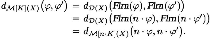
• 2. For multisets $\varphi ,\varphi '\in \mathcal {M}[K](X)$, by the previous item:

  

• 3. For multisets $\varphi ,\varphi '\in \mathcal {M}[K](X)$ and $\psi ,\psi '\in \mathcal {M}[L](X)$, using Lemma 2 (8),

  

• 4. Let $f:X \rightarrow Y$ be M-Lipschitz. We use that frequentist learning is an isometry and a natural transformation $\mathcal {M}[K] \Rightarrow \mathcal {D}$. For multisets $\varphi ,\varphi '\in \mathcal {M}[K](X)$,

  

• 5. The map is $\frac{1}{K}$-Lipschitz since for $\boldsymbol{y}, \boldsymbol{y'} \in X^{K}$,

  

• 6. For fixed $\varphi , \varphi '\in \mathcal {M}[K](X)$, take arbitrary and . Then:

  

  Since this holds for all , we get an inequaltiy , see Definition 3. This inequality is an actual equality since , and thus , is $\frac{1}{K}$-Lipschitz:

  

  

6 Multinomial drawing is isometric

Multinomial draws are of the draw-and-replace kind. This means that a drawn ball is returned to the urn, so that the urn remains unchanged. Thus we may use a distribution $\omega \in \mathcal {D}(X)$ as urn. For a draw size number $K\in \mathbb {N}$, the multinomial distribution on multisets / draws of size K can be defined via accumulated sequences of draws:

(10)

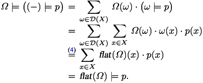
We recall that is the number of sequences that accumulate to a multiset / draw $\varphi \in \mathcal {M}[K](X)$. A basic result from [8, Prop. 3] is that applying frequentist learning to the draws yields the original urn:

(11)

We can now formulate and prove our first isometry result.

Theorem 1

Let X be an arbitrary metric space (of colours), and $K>0$ be a positive natural (draw size) number. The multinomial channel

is an isometry. This involves the Wasserstein metric (8) for distributions over X on the domain $\mathcal {D}(X)$, and the Wasserstein metric for distributions over multisets of size K, with their Wasserstein metric (9), on the codomain $\mathcal {D}\big (\mathcal {M}[K](X)\big )$.

Proof

Let distributions $\omega ,\omega '\in \mathcal {D}(X)$ be given. The map is short since:

There is also an inequality in the other direction, via:

The latter inequality follows from the fact that frequentist learning is short, see Lemma 3 (1), and that Kleisli extension is thus short too, see Lemma 2 (6).

Example 3

Consider the following two distributions $\omega ,\omega '\in \mathcal {D}(\mathbb {N})$.

$$ \begin{array}{lll} \omega = \frac{1}{3}|{}0{}\rangle + \frac{2}{3}|{}2{}\rangle & \quad \text{ and } \quad \omega ' = \frac{1}{2}|{}1{}\rangle + \frac{1}{2}|{}2{}\rangle & \quad \text{ with } \quad d(\omega ,\omega ') = \frac{1}{2}. \end{array} $$

This distance $d(\omega ,\omega ')$ involves the standard distance on $\mathbb {N}$, using the optimal coupling $\frac{1}{3}|{}0, 1{}\rangle + \frac{1}{6}|{}2, 1{}\rangle + \frac{1}{2}|{}2, 2{}\rangle \in \mathcal {D}\big (\mathbb {N}\times \mathbb {N}\big )$.

We take draws of size $K=3$. There are 10 multisets of size 3 over $\{0,1,2\}$:

$$ \begin{array}{c} \varphi _{1} = 3|{}0{}\rangle \qquad \varphi _{2} = 2|{}0{}\rangle + 1|{}1{}\rangle \qquad \varphi _{3} = 1|{}0{}\rangle + 2|{}1{}\rangle \qquad \varphi _{4} = 3|{}1{}\rangle \\ \varphi _{5} = 2|{}0{}\rangle + 1|{}2{}\rangle \qquad \varphi _{6} = 1|{}0{}\rangle + 1|{}1{}\rangle + 1|{}2{}\rangle \qquad \varphi _{7} = 2|{}1{}\rangle + 1|{}2{}\rangle \\ \varphi _{8} = 1|{}0{}\rangle + 2|{}2{}\rangle \qquad \varphi _{9} = 1|{}1{}\rangle + 2|{}2{}\rangle \qquad \varphi _{10} = 3|{}2{}\rangle . \end{array} $$

These multisets occur in the following multinomial distributions of draws of size 3.

The optimal coupling $\tau \in \mathcal {D}\big (\mathcal {M}[3](\mathbb {N}) \times \mathcal {M}[3](\mathbb {N})\big )$ between these two multinomial distributions is:

We compute the distance between the multinomial distributions, using $d_{\mathcal {M}} = d_{\mathcal {M}[3](\mathbb {N})}$.

As predicted in Theorem 1, this distance coincides with the distance $d(\omega ,\omega ') = \frac{1}{2}$ between the original urn distributions. One sees that the computation of the distance between the draw distributions is more complex, involving ‘Wasserstein over Wasserstein’.

7 Hypergeometric drawing is isometric

We start with some preparatory observations on probabilistic projection and drawing.

Lemma 4

For a metric space X and a number K, consider the probabilistic projection-delete and probabilistic draw-delete channels.

They are defined via deletion of elements from sequences and from multisets:

Then:

• 1. ;

• 2.   ;

• 3.   is $\frac{K}{K+1}$-Lipschitz, and thus short;

• 4.   is an isometry.

Proof

The first point is easy and the second one is [8, Lem. 5 (ii)].

• 3. For $\boldsymbol{x}, \boldsymbol{y} \in X^{K+1}$, via Lemma 2 (8) and (4),

  

• 4. Via item 1 we get:

  

  Now we can show that is short: for $\psi ,\psi '\in \mathcal {M}[K+1](X)$

  

  For the reverse inequality we use item 2 and the fact that is a short:

  

  

The hypergeometric channel , for urn size $L \ge K$, where K is the draw size, is an iteration of draw-delete’s, see [8, Thm. 6]:

(12)

where $\left( {\begin{array}{c}\upsilon \\ \varphi \end{array}}\right) {:}{=}\prod _{x\in X} \left( {\begin{array}{c}\upsilon (x)\\ \varphi (x)\end{array}}\right)$.

Theorem 2

The hypergeometric channel defined in (12), for $L\ge K$, is an isometry.

Proof

We see in (12) that is a (channel) iteration of isometries , and thus of short maps; hence it it short itself. Via iterated use of Lemma 4 (2) we get . This gives the inequality in the other direction, like in the proof of Lemma 4 (2):

The very beginning of this paper contains an illustration of this result, for urns over the set of colours $C = \{R,G,B\}$, considered as a discrete metric space.

8 Pólya drawing is isometric

Hypergeometric distributions use the draw-delete mode: a drawn ball is removed from the urn. The less well-known Pólya draws [7] use the draw-add mode. This means that a drawn ball is returned to the urn, together with another ball of the same colour (as the drawn ball). Thus, with hypergeometric draws the urn decreases in size, so that only finitely many draws are possible, whereas with Pólya draws the urn grows in size, and the drawing may be repeated arbitrarily many times. As a result, for Pólya distributions we do not need to impose restrictions on the size K of draws. We do have to restrict draws from urn $\upsilon$ to multisets $\varphi \in \mathcal {M}[K](X)$ with since we can only draw balls of colours that are in the urn. Pólya distributions are formulated in terms of multi-choose binomials $\left( {}\left( {\begin{array}{c}n\\ m\end{array}}\right) {}\right) {:}{=}\left( {\begin{array}{c}n+m-1\\ m\end{array}}\right) = \frac{(n+m-1)!}{m!\cdot (n-1)!}$, for $n>0$. This multi-choose number $\left( {}\left( {\begin{array}{c}n\\ m\end{array}}\right) {}\right)$ is the number of multisets of size m over a set with n elements, see [9, 10] for details.

(13)

where .

Theorem 3

Each Pólya channel , for urn and draw sizes $L > 0, K > 0$, is an isometry.

Proof

One inequality follows by exploiting the equation like in previous sections. The reverse inequality, for shortness, involves a draw-store-add channel of the form:

defined as:

With some effort one shows that this channel is short and that the Pólya channel can be expressed via iterated draw-store-add’s, namely as:

where $\textbf{0}\in \mathcal {M}[0](X)$ is the empty multiset. This makes the Pólya channel short, and thus an isometry.

We illustrate that the Pólya channel is an isometry.

Example 4

We take as space of colours $X = \{0, 10, 50\} \subseteq \mathbb {N}$ with two urns:

$$ \begin{array}{ll} \upsilon _{1} = 3|{}0{}\rangle + 1|{}10{}\rangle & \qquad \upsilon _{2} = 1|{}0{}\rangle + 2|{}10{}\rangle + 1|{}50{}\rangle . \end{array} $$

The distance between these urns is 15, via the optimal coupling $1|{}0, 0{}\rangle + 2|{}0, 10{}\rangle + 1|{}10, 50{}\rangle$, yielding $\frac{1}{4}\cdot (0-0) + \frac{1}{2}\cdot (10-0) + \frac{1}{4}\cdot (50-10) = 5 + 10 = 15$.

We look at Pólya draws of size $K=2$. This gives distributions:

We compute the distance between these two distributions via the last formulation in (8), using the optimal short factor $p:\mathcal {M}[2](X) \rightarrow \mathbb {R}_{\ge 0}$ given by:

Then:

As predicted by Theorem 3, the distance between the Pólya distributions then coincides with the distance between the urns:

9 Conclusions

Category theory provides a fresh look at the area of probability theory, see e.g. [5] or [10] for an overview. Its perspective allows one to formulate and prove new results. This paper demonstrates that draw operations, viewed as (Kleisli) maps, are incredibly well-behaved: they preserve Wasserstein distances. Such distances on urns filled with coloured balls are relatively simple, starting from a ‘ground’ metric on the set of colours. But on draw distributions, the distances involve Wasserstein-over-Wasserstein. This paper concentrates on drawing from an urn. A natural question is whether other probabilistic operations, as Kleisli maps, preserve distance. This is a topic for further investigation.

References

F. van Breugel. An introduction to metric semantics: operational and denotational models for programming and specification languages. Theor. Comp. Sci., 258(1-2):1–98, 2001. https://doi.org/10.1016/S0304-3975(00)00403-5.
H. Brezis. Remarks on the Monge-Kantorovich problem in the discrete setting. Comptes Rendus Mathematique, 356(2):207–213, 2018. https://doi.org/10.1016/j.crma.2017.12.008.
Y. Deng and W. Du. The Kantorovich metric in computer science: A brief survey. In C. Baier and A. di Pierro, editors, Quantitative Aspects of Programming Languages, number 253(3) in Elect. Notes in Theor. Comp. Sci., pages 73–82. Elsevier, Amsterdam, 2009. https://doi.org/10.1016/j.entcs.2009.10.006.
J. Desharnais, V. Gupta, R. Jagadeesan, and P. Panangaden. Metrics for labelled Markov processes. Theor. Comp. Sci., 318:232–354, 2004.
T. Fritz. A synthetic approach to Markov kernels, conditional independence, and theorems on sufficient statistics. Advances in Math., 370:107239, 2020. https://doi.org/10.1016/J.AIM.2020.107239.
T. Fritz and P. Perrone. A probability monad as the colimit of spaces of finite samples. Theory and Appl. of Categories, 34(7):170–220, 2019. https://doi.org/10.48550/arXiv.1712.05363.
F. Hoppe. Pólya-like urns and the Ewens’ sampling formula. Journ. Math. Biology, 20:91–94, 1984. https://doi.org/10.1007/BF00275863.
B. Jacobs. From multisets over distributions to distributions over multisets. In Logic in Computer Science. IEEE, Computer Science Press, 2021. https://doi.org/10.1109/lics52264.2021.9470678.
B. Jacobs. Urns & tubes. Compositionality, 4(4), 2022. https://doi.org/10.32408/compositionality-4-4.
B. Jacobs. Structured probabilitistic reasoning. Book, in preparation, see http://www.cs.ru.nl/B.Jacobs/PAPERS/ProbabilisticReasoning.pdf, 2023.
B. Jacobs and A. Westerbaan. Distances between states and between predicates. Logical Methods in Comp. Sci., 16(1), 2020. See https://lmcs.episciences.org/6154.
L. Kantorovich and G. Rubinshtein. On a space of totally additive functions. Vestnik Leningrad Univ., 13:52–59, 1958.
J. Matouĕk and B. Gärtner. Understanding and Using Linear Programming. Springer Verlag, Berlin, 2006. https://doi.org/10.1007/978-3-540-30717-4.
Y. Rubner, C. Tomasi, and L. Guibas. The Earth Mover’s Distance as a metric for image retrieval. Int. Journ. of Computer Vision, 40:99–121, 2000. https://doi.org/10.1023/A:1026543900054.
C. Villani. Optimal Transport — Old and New. Springer, Berlin Heidelberg, 2009. https://doi.org/10.1007/978-3-540-71050-9.
G. Wyszecki and W. Stiles. Color Science: Concepts and Methods, Quantitative Data and Formulae. Wiley, 1982.
Acknowledgments
Thanks are due to the anonymous reviewers for their detailed comments that improved an earlier version of this work.
Author information
Authors and Affiliations
Corresponding author
Editor information
Editors and Affiliations
Rights and permissions
Open Access This chapter is licensed under the terms of the Creative Commons Attribution 4.0 International License (http://creativecommons.org/licenses/by/4.0/), which permits use, sharing, adaptation, distribution and reproduction in any medium or format, as long as you give appropriate credit to the original author(s) and the source, provide a link to the Creative Commons license and indicate if changes were made.
The images or other third party material in this chapter are included in the chapter's Creative Commons license, unless indicated otherwise in a credit line to the material. If material is not included in the chapter's Creative Commons license and your intended use is not permitted by statutory regulation or exceeds the permitted use, you will need to obtain permission directly from the copyright holder.
Copyright information
© 2024 The Author(s)
About this paper
Cite this paper
Jacobs, B. (2024). Drawing from an Urn is Isometric. In: Kobayashi, N., Worrell, J. (eds) Foundations of Software Science and Computation Structures. FoSSaCS 2024. Lecture Notes in Computer Science, vol 14574. Springer, Cham. https://doi.org/10.1007/978-3-031-57228-9_6
Download citation
DOI: https://doi.org/10.1007/978-3-031-57228-9_6
Published:
Publisher Name: Springer, Cham
Print ISBN: 978-3-031-57227-2
Online ISBN: 978-3-031-57228-9
eBook Packages: Computer ScienceComputer Science (R0)