Tighter Construction of Tight Büchi Automata

Abstract

Tight automata are useful in providing the shortest counterexample in LTL model checking and also in constructing a maximally satisfying strategy in LTL strategy synthesis. There exists a translation of LTL formulas to tight Büchi automata and several translations of Büchi automata to equivalent tight Büchi automata. This paper presents another translation of Büchi automata to equivalent tight Büchi automata. The translation is designed to produce smaller tight automata and it asymptotically improves the best-known upper bound on the size of a tight Büchi automaton equivalent to a given Büchi automaton. We also provide a lower bound, which is more precise than the previously known one. Further, we show that automata reduction methods based on quotienting preserve tightness. Our translation was implemented in a tool called Tightener. Experimental evaluation shows that Tightener usually produces smaller tight automata than the translation from LTL to tight automata known as CGH.

Marek Jankola–This research was conducted partly during Master’s studies of M. Jankola at Masaryk University in Brno, Czechia.

1 Introduction

When a model checking algorithm decides that a given system violates a given specification, a counterexample showing the undesired system behavior is produced. If the system has only finitely many states and it violates the specification given by a formula of Linear Temporal Logic (LTL) or directly by a Büchi automaton accepting all erroneous behaviors, there exists a counterexample of the form $u.v^\omega$ called lasso-shaped or ultimately periodic. A serious research effort has been devoted to algorithms that produce short counterexamples, where the length of a counterexample $u.v^\omega$ is given by |uv| [7, 12, 13, 15, 19, 22, 24].

In 2005, Schuppan and Biere [24] defined tight Büchi automata, where each lasso-shaped word accepted by such an automaton is accepted by a lasso-shaped run of the same length. Hence, the product of a tight automaton $\mathcal {A}$ with an arbitrary transition system accepts the shortest lasso-shaped behavior of the system that is in the language of $\mathcal {A}$ by the shortest lasso-shaped accepting run. This property makes tight automata very useful for automata-based model checking algorithms looking for shortest counterexamples, which was the original motivation for the definition. Tight automata found another application in autonomous robot action planning, where they are used in the algorithm synthesizing a maximally satisfying discrete control strategy while taking into account that the robot’s action executions may fail [27].

There exist only few algorithms producing tight automata. The oldest is the translation of LTL formulas into generalized Büchi automata introduced by Clarke, Grumberg, and Hamaguchi [6] in 1994. The fact that this translation creates tight automata was shown about 10 years later by Schuppan and Biere [24], who named the translation CGH. They extended the translation to handle also past LTL operators and implemented it. The implementation produces automata in symbolic representation suitable for the model checker NuSMV [5].

There are also two constructions transforming Büchi automata into tight Büchi automata. The first was introduced by Schuppan [23] and it accepts even generalized Büchi automata as input. For a (non-generalized) Büchi automaton with n states, this construction creates a tight automaton with $\mathcal {O}((\sqrt{2}n)^{2n})$ states. The second (and completely different) construction was introduced by Ehlers [13] and it produces tight automata of size $2^{\mathcal {O}(n^2)}$ states. Kupferman and Vardi [20] provided the lower bound $2^{\varOmega (n)}$ as a side result when analyzing counterexamples of safety properties. We are not aware of any implementation of these constructions.

This paper presents another construction transforming Büchi automata to tight Büchi automata. More precisely, our construction accepts (state-based) Büchi automata (BA) or transition-based Büchi automata (TBA) and produces tight BA or tight TBA. The construction is similar to the one of Schuppan [23], but it produces less states: while Schuppan’s construction creates states that represent a sequence of up to 2n states of the original automata, our construction creates states representing at most n states of the original automaton and these n states are pairwise different (potentially with a single exception). The construction gives us an upper bound in $\mathcal {O}(n!\cdot n^3)$ which is strictly below both $\mathcal {O}((\sqrt{2}n)^{2n})$ and $2^{\mathcal {O}(n^2)}$. We also provide a lower bound in $\varOmega (\frac{n-1}{2}!)$ for any transformation of BA into equivalent tight BA or TBA and a lower bound in $\varOmega ((n-1)!)$ for any transformation of TBA into equivalent tight BA or TBA. Note that the lower bound $\varOmega (\frac{n-1}{2}!)$ is strictly above the previous lower bound $2^{\varOmega (n)}$. Additionally, we show that tight automata can be reduced by quotienting with use of an arbitrary good-for-quotienting (GFQ) relation [8] and the resulting automaton is equivalent and tight.

Our paper also delivers some practical results. The tightening algorithm has been implemented in a tool called Tightener. The tool can be easily combined with other automata tools as it accepts and produces automata in the HOA format [2]. Furthermore, it also accepts LTL formulas on input. When Tightener receives an LTL formula, it calls the LTL to TBA translation of Spot [10] as the first step. We compare Tightener against the CGH translation as this is (as far as we know) the only other implemented algorithm producing tight automata. Our experimental evaluation shows that tight automata produced by CGH usually have more states than the ones by Tightener.

Contributions of the paper. The paper brings the following contributions:

• a construction transforming BA/TBA into tight BA/TBA with the lowest theoretical upper bound on the rise of the state space so far,

• lower bounds on any transformation of BA or TBA into equivalent tight BA/TBA that are currently the highest lower bounds,

• a proof that the automata reduction based on quotienting preserves tightness,

• a tool Tightener producing tight BA/TBA from LTL formulas or BA/TBA,

• an experimental comparison of tight automata by Tightener and CGH.

Structure of the paper. The following section introduces the basic terminology used in the paper. Section 3 formulates some observations crucial for our tightening construction, which is then presented in Section 4 together with the implied upper bound. Section 5 shows the lower bounds on the tightening process. The postprocessing of tight automata is discussed in Section 6. Section 7 describes the implementation of our tightening construction in Tightener and Section 8 compares it to the CGH translation in terms of the sizes of produced tight automata. Finally, Section 9 concludes the paper.

2 Preliminaries

A transition-based Büchi automaton (TBA) is a tuple $\mathcal {A}=(Q,\varSigma ,\delta ,I,\delta _F)$, where

• Q is a finite set of states,

• $\varSigma$ is a finite alphabet,

• $\delta \subseteq Q\times \varSigma \times Q$ is a transition relation,

• $I\subseteq Q$ is a set of initial states, and

• $\delta _F\subseteq \delta$ is a set of accepting transitions.

A run of $\mathcal {A}$ over an infinite word $u=u_0u_1\ldots \in \varSigma ^\omega$ is an infinite sequence $\rho =(q_0,u_0,q_1)(q_1,u_1,q_2)\ldots \in \delta ^\omega$ of consecutive transitions starting in an initial state $q_0\in I$. By $\rho _i$, we denote the transition $(q_i, u_i, q_{i+1})$ from $\rho$. A run $\rho$ is accepting if $(q_i,u_i,q_{i+1})\in \delta _F$ holds for infinitely many i. An automaton accepts a word u if there exists an accepting run over this word. A language of automaton $\mathcal {A}$ is the set $L(\mathcal {A})$ of all words in $\varSigma ^\omega$ accepted by $\mathcal {A}$. Automata $\mathcal {A},\mathcal {B}$ are equivalent if $L(\mathcal {A})=L(\mathcal {B})$.

A transition $(p,a,q)\in \delta$ is also denoted as $p\xrightarrow {a}_{}q$. In graphical representation, accepting transitions are these marked with the blue dot . In the following, word without any adjective refers to an infinite word. A path in $\mathcal {A}$ from a state $q_0$ to a state $q_n$ over a finite word $r=r_0r_1\ldots r_{n-1}\in \varSigma ^*$ is a finite sequence $\sigma =(q_0,r_0,q_1)(q_1,r_1,q_2)\ldots (q_{n-1},r_{n-1},q_{n})\in \delta ^n$ of consecutive transitions. We refer to a first state $q_0$ of a path as to initial state of the path. We naturally extend the notation for transitions and write that the path $\sigma$ has the form $q_0\xrightarrow {r}_{}q_n$. If such a path exists, we say that $q_n$ is reachable from $q_0$ over r. For a word or a run $u=u_0u_1\ldots$, by $u_{i..}$ we denote its suffix $u_iu_{i+1}\ldots$ and by $u_{i,j}$, for $i < j$, we denote its subpart $u_iu_{i+1}\ldots u_{j-1}$.

The paper intensively works with lasso-shaped words and runs, which are sequences of the form $s.l^{\omega }$, where s is called a stem and $l\ne \varepsilon$ is called a loop. Further, s is a minimal stem and l is a minimal loop of a lasso-shaped sequence $u=s.l^\omega$ if for each $s',l'$ satisfying $u=s'.l'^\omega$ it holds $|s|+|l|\le |s'|+|l'|$.

Lemma 1

For each lasso-shaped sequence, there exist a unique minimal stem and a unique minimal loop.

Proof

The existence of some minimal stem and loop for each lasso-shaped sequence u is obvious. We prove its uniqueness by contradiction. Assume that there are two different pairs s, l and $s',l'$ of minimal stem and loop, which implies that $u=s.l^\omega =s'.l'^\omega$ and $|s|+|l|=|s'|+|l'|$. Without loss of generality, assume that $|s| < |s'|$ and $|l| > |l'|$. As $|s|+|l|=|s'|+|l'|$, we get $l^{\omega } = u_{|s|+|l|..} = u_{|s'|+|l'|..}=l'^{\omega }$ and thus $s.l^{\omega } = s.l'^{\omega }$. However, this is a contradiction with the minimality of s, l and $s',l'$ as $|s| + |l'|<|s|+|l|=|s'|+|l'|$.    $\square$

The minimal stem and the minimal loop of a lasso-shaped sequence u is denoted by $minS (u)$ and $minL (u)$, respectively. Moreover, we set $| minSL (u)|=| minS (u)|+| minL (u)|$ and call it the size of u.

If $\rho$ is a lasso-shaped run over a word u, then u is a lasso-shaped word such that $| minS (u)|\le | minS (\rho )|$ and $| minL (u)|\le | minL (\rho )|$.

A TBA $\mathcal {A}$ is tight [24] iff for each lasso-shaped word $u\in L(\mathcal {A})$ there exists an accepting lasso-shaped run $\rho$ satisfying $| minSL (u)|=| minSL (\rho )|$. We call such runs tight.

A state-based Büchi automaton (BA) is a tuple $\mathcal {A}=(Q,\varSigma ,\delta ,I,F)$, where $Q,\varSigma ,\delta ,I$ have the same meaning as in a TBA and $F\subseteq Q$ is a set of accepting states. The definition of all terms is the same as for TBA with the exception of accepting run. A run $\rho =(q_0,u_0,q_1)(q_1,u_1,q_2)\ldots \in \delta ^\omega$ is accepting if $q_i\in F$ for infinitely many i. Note that BA can be seen as a special case of TBA as each BA can be easily transformed into an equivalent TBA only by replacing its accepting states F with the set of transitions $\delta _F$ leading to these states, i.e., $\delta _F=\{(p,a,q)\in \delta \mid q\in F\}$.

Finally, a (state-based) generalized Büchi automaton (GBA) is a tuple $\mathcal {A}=(Q,\varSigma ,\delta ,I,\mathcal {F})$, where $Q,\varSigma ,\delta ,I$ have the same meaning as in a TBA and $\mathcal {F}=\{F_1,\ldots ,F_k\}$ is a finite set of sets $F_j\subseteq Q$. The definition of all terms is the same as for TBA, except for an accepting run. A run $\rho =(q_0,u_0,q_1)(q_1,u_1,q_2)\ldots \in \delta ^\omega$ is accepting if for each $F_j\in \mathcal {F}$ there exist infinitely many i satisfying $q_i\in F_j$.

3 Observations

First of all, we explain why our definition of TBA considers multiple initial states. As every TBA can be transformed into an equivalent TBA with a single initial state, some definitions of TBA consider exactly one initial state. However, a tight TBA with one initial state would have only a restricted expressive power. Indeed, each TBA can be transformed to an equivalent tight TBA with multiple initial states (as we show in the following section), but there exist TBA that cannot be transformed into equivalent tight TBA with a single initial state.

Lemma 2

There exists a TBA such that there is no equivalent tight TBA with a single initial state.

Proof

Let $\mathcal {A}$ be the TBA in Figure 1 (left). For the sake of contradiction, assume that there is a tight TBA $\mathcal {B}$ with one initial state $q_0$ and equivalent to $\mathcal {A}$. Then $\mathcal {B}$ must accept $a^{\omega }$ and $b^{\omega }$. Furthermore, since $| minSL (a^{\omega })| = | minSL (b^{\omega })| = 1$ and $\mathcal {B}$ is tight, there must exist accepting self-loops over a and b in $q_0$. However, $\mathcal {B}$ then accepts for instance $a.b^{\omega }\notin L(\mathcal {A})$, which is a contradiction.    $\square$

Fig. 1.

TBA with a single initial state (left) and an equivalent tight TBA with two initial states (right).

As the (un)tightness of an automaton depends purely on lasso-shaped words accepted by the automaton and the corresponding accepting runs, we turn our attention to these words. We start with the definition of significant positions in a lasso-shaped word u as positions i where $u_{i..}= minL (u)^\omega$. Formally, we set

$$ Sign ^{}(u)=\{k,k+o,k+2o,k+3o,\ldots \}$$

where $k=| minS (u)|$ and $o=| minL (u)|$. We first prove that for every lasso-shaped word u accepted by a TBA, there exists a lasso-shaped accepting run over u.

Lemma 3

Let $\mathcal {A}$ be a TBA. For each lasso-shaped word $u\in L(\mathcal {A})$ there exists a lasso-shaped accepting run over u of the form $\tau .\pi ^\omega$, where

• $\tau$ is a path over $minS (u). minL (u)^i$ for some $i\ge 0$ and

• $\pi$ is a path over $minL (u)^k$ for some $k>0$.

Proof

Let $u\in L(\mathcal {A})$ be a lasso-shaped word and $\rho =(q_0,u_0,q_1)(q_1,u_1,q_2)\ldots$ be an accepting run of $\mathcal {A}$ over this word. We focus on states of this run at significant positions, i.e., states $q_k,q_{k+o},q_{k+2o},\ldots$ where $k=| minS (u)|$ and $o=| minL (u)|$. The run and its states at significant positions are depicted in Figure 2. Since $\mathcal {A}$ has finitely many states, there are positions $p_1,p_2\in Sign ^{}(u)$ such that $p_1<p_2$, $q_{p_1} = q_{p_2}$, and path $\rho _{p_1,p_2}$ contains an accepting transition. We set $\tau =\rho _{0,p_1}$ and $\pi =\rho _{p_1,p_2}$. As $p_1,p_2$ are significant positions, $\tau$ is a path over $minS (u). minL (u)^i$ for some $i\ge 0$ and $\pi$ is a path over $minL (u)^k$ for some $k>0$. As $q_{p_1} = q_{p_2}$ and $\pi$ contains an accepting transition, $\tau .\pi ^\omega$ is an accepting run over u.   $\square$

Fig. 2.

A run over a lasso-shaped word $u=u_0u_1\ldots$ with states at significant positions typeset in red.

Fig. 3.

An example of a TBA that is not tight.

Once we know that each lasso-shaped word $u\in L(\mathcal {A})$ has a lasso-shaped accepting run, we also know that there exists at least one accepting lasso-shaped run $\rho$ over u with the minimal size $| minSL (\rho )|$. We call such runs minimal. For example, consider the word $b.(abc)^\omega$ accepted by the automaton in Figure 3. The minimal run for this word is $\tau .\pi ^\omega$ with the following minimal stem $\tau$ and minimal loop $\pi$.

Now we formulate and prove Lemma 4, which says that each minimal run $\rho$ has a specific property regarding repetition of states. The property considers states of $\rho$ at the positions at least $| minS (u)|$ and less than $| minSL (\rho )|$. The property says that there cannot be the same state twice on the considered positions from which the same suffix of u is read. It can be illustrated on the minimal run $\tau .\pi ^\omega$ mentioned above. If we write the states of this run such that the states reading the same suffix of u are vertically aligned (see Table 1), the considered states in each column are pairwise different.

Table 1. Illustration of the property formulated in Lemma 4. Unconsidered states are struck through and states at significant positions are typeset in red.

Lemma 4

Let $\mathcal {A}$ be a TBA and $\rho =(q_0,u_0,q_1)(q_1,u_1,q_2)\ldots$ be a minimal run over a lasso-shaped word $u\in L(\mathcal {A})$. For each $| minS (u)|\le m<l<| minSL (\rho )|$ satisfying $u_{m..}=u_{l..}$ it holds that the states $q_m$ and $q_l$ are different.

Proof

Let $\mathcal {A}$ be a TBA and $\rho =(q_0,u_0,q_1)(q_1,u_1,q_2)\ldots$ be a minimal run over a lasso-shaped word $u\in L(\mathcal {A})$. For the sake of contradiction, assume that there are positions $| minS (u)|\le m<l<| minSL (\rho )|$ such that $u_{m..} = u_{l..}$ and $q_m = q_l$. We will show that there exists another lasso-shaped accepting run $\rho '$ over u of a smaller size than $\rho$. This will give us a contradiction with the minimality of $\rho$.

We start with the case that the path $\rho _{m,l}$ from $q_m$ to $q_l$ contains an accepting transition. The equation $u_{m..} = u_{l..}$ implies that $u_{m..} = u_{l..} = (u_{m,l})^\omega$. Hence, $\rho ' = \rho _{0,m}.(\rho _{m,l})^{\omega }$ is a lasso-shaped accepting run over u. Moreover, the size of $\rho '$ is smaller than the size of $\rho$ as $| minSL (\rho ')|\le |\rho _{0,m}|+|\rho _{m,l}|=l<| minSL (\rho )|$.

Now we solve the case when there is no accepting transition in the path $\rho _{m,l}$. First, assume that $\rho _{m,l}$ is completely included in the minimal stem of $\rho$, i.e., $m<l \le | minS (\rho )|$. Then we simply exclude $\rho _{m,l}$ from the stem and get an accepting lasso-shaped run $\rho '$ over u, which has a shorter stem than $\rho$. Second, assume that $\rho _{m,l}$ is partly in the minimal stem and partly in the minimal loop of $\rho$, i.e., $m < | minS (\rho )| < l$. Let $\rho '=\rho _{0,m}.\rho _{l..}$ be the run $\rho$ without the path $\rho _{m,l}$. Note that $\rho '$ is again an accepting run over u as $u_{m..} = u_{l..}$. As $\rho$ is lasso-shaped, we know that $\rho _{l..} = (\rho _{l,l+| minL (\rho )|})^{\omega }$. Hence, $\rho '=\rho _{0,m}.(\rho _{l,l+| minL (\rho )|})^{\omega }$ is also lasso-shaped. Moreover, the size of $\rho '$ is smaller than the size of $\rho$ as $| minSL (\rho ')|\le m+| minL (\rho )|<| minS (\rho )|+| minL (\rho )|=| minSL (\rho )|$. Finally, assume that $\rho _{m,l}$ is completely included in the minimal loop of $\rho$, i.e., $| minS (\rho )|\le m<l$. Then we exclude $\rho _{m,l}$ from the minimal loop of $\rho$ and get an accepting run $\rho '=\rho _{0,| minS (\rho )|}.(\rho _{| minS (\rho )|,m}.\rho _{l,| minSL (\rho )|})^\omega$ of a smaller size than $\rho$. We need to show that $\rho '$ accepts u. The run $\rho '$ accepts the word $u'=u_{0,| minS (\rho )|}.(u_{| minS (\rho )|,m}.u_{l,| minSL (\rho )|})^\omega =u_{0,m}.(u_{l,| minSL (\rho )|}.u_{| minS (\rho )|,m})^\omega$. As $u_{| minS (\rho )|,m}=u_{| minSL (\rho )|,m+| minL (\rho )|}$, we get $u'=u_{0,m}.(u_{l,m+| minL (\rho )|})^\omega$. Further, $u_{m..}=u_{l..}=u_{m+| minL (\rho )|..}$ implies $u_{m..}=u_{l..}=(u_{l,m+| minL (\rho )|})^\omega$ and thus $u'=u_{0,m}.u_{m..}=u$.    $\square$

The next lemma shows that each minimal run over u can be denoted as a lasso-shaped structure build from one path over $minS (u)$ and at most n paths over $minL (u)$, where n is the number of states in the automaton. For example, the minimal run $\tau .\pi ^\omega$ over $b.(abc)^\omega$ presented above can be also denoted as $\pi _0\pi _1\pi _2.(\pi _3\pi _4\pi _5)^\omega$, where the paths $\pi _i$ are defined as follows.

Note that the stem $\pi _0\pi _1\pi _2$ is not the minimal stem and $\pi _3\pi _4\pi _5$ is not the minimal loop of the minimal run $\tau .\pi ^\omega$. Further, note that the paths $\pi _1,\ldots ,\pi _5$ start in the considered states at significant positions, which are typeset in red and not struck through in Table 1.

Lemma 5

Let $\mathcal {A}$ be a TBA with n states and $\rho$ be a minimal run over a lasso-shaped word $u\in L(\mathcal {A})$. Then $\rho$ can be denoted as $\pi _0\pi _1\ldots \pi _i.(\pi _{i+1}\pi _{i+2}\ldots \pi _k)^\omega$, where $\pi _0$ is a path over $minS (u)$, $\pi _1,\pi _2,\ldots ,\pi _k$ are paths over $minL (u)$, and $0\le i<k\le n$. Moreover, $| minSL (\rho )|\le |\pi _0\pi _1\ldots \pi _k|<| minSL (\rho )|+| minL (u)|$ and the last $|\pi _0\pi _1\ldots \pi _k|-| minSL (\rho )|$ transitions of $\pi _k$ and $\pi _i$ are identical.

Proof

Let $\mathcal {A}$ be a TBA with n states and $\rho =(q_0,u_0,q_1)(q_1,u_1,q_2)\ldots$ be a minimal run over a lasso-shaped word $u\in L(\mathcal {A})$. The lasso shape of $\rho$ implies that $\rho _{| minS (\rho )|..}=\rho _{| minSL (\rho )|..}$ and thus also $u_{| minS (\rho )|..}=u_{| minSL (\rho )|..}$. This means that $| minL (\rho )|=j\cdot | minL (u)|$ for some $j>0$.

Let $i\ge 0$ be the smallest number such that $minS (u). minL (u)^i$ is at least as long as $minS (\rho )$. As $| minL (\rho )|=j\cdot | minL (u)|$, then $k=i+j$ is the smallest number such that $minS (u). minL (u)^k$ is at least as long as $minS (\rho ). minL (\rho )$. Let $p_1,p_2,\ldots ,p_k,p_{k+1}$ be the first $k+1$ significant positions in u. We set $\pi _0=\rho _{0,p_1}$ to be the prefix of $\rho$ over $minS (u)$ and, for each $1\le l\le k$, we set $\pi _l=\rho _{p_l,p_{l+1}}$ to be the l-th successive subpart of $\rho$ over $minL (u)$. The definition of k implies that $| minSL (\rho )|\le |\pi _0\pi _1\ldots \pi _k|<| minSL (\rho )|+| minL (u)|$.

We have $\pi _0\pi _1\ldots \pi _k= minS (\rho ). minL (\rho ).\pi '$, where $\pi '$ is a prefix of $minL (\rho )$ such that $0\le |\pi '|=|\pi _0\pi _1\ldots \pi _k|-| minSL (\rho )|<|\pi _k|$. As $|\pi _{i+1}\pi _{i+2}\ldots \pi _k|=j\cdot | minL (u)|=| minL (\rho )|$, we get that $\pi _0\pi _1\ldots \pi _i= minS (\rho ).\pi '$ and this means that $\pi _k$ and $\pi _i$ have the same suffix $\pi '$ of the length $|\pi '|=|\pi _0\pi _1\ldots \pi _k|-| minSL (\rho )|$. Note that this holds also in the case when $i=0$ because this situation implies that $\pi _0= minS (\rho )$ and thus $\pi '=\varepsilon$.

As $\pi _0\pi _1\ldots \pi _i= minS (\rho ).\pi '$ and $\pi _0\pi _1\ldots \pi _k= minS (\rho ). minL (\rho ).\pi '$, we get that there exists $\pi ''$ such that $minL (\rho )=\pi '.\pi ''$. Then

$$\pi _0\pi _1\ldots \pi _i.(\pi _{i+1}\pi _{i+2}\ldots \pi _k)^\omega = minS (\rho ).\pi '.(\pi ''.\pi ')^\omega = minS (\rho ).(\pi '.\pi '')^\omega =\rho .$$

It remains to show that $k\le n$. For each significant position $p_l$ such that $1\le l\le k$, it holds that $| minS (u)|\le p_l<| minSL (\rho )|$ and $u_{p_l..}= minL (u)^\omega$. Lemma 4 says that states of the run $\rho$ at positions $p_1,p_2,\ldots ,p_k$ are pairwise different. Hence, $k\le n$.   $\square$

4 Tightening construction and upper bound

Our tightening construction extends a given automaton $\mathcal {A}$ with new states and transitions to make it tight. Let n be the number of states in $\mathcal {A}$. Lemmata 3–5 imply that for each lasso-shaped word $u\in L(\mathcal {A})$, there exists an accepting run $\rho =\pi _0\pi _1\ldots \pi _i.(\pi _{i+1}\pi _{i+2}\ldots \pi _k)^\omega$ over u where $0\le i<k\le n$, $\pi _0$ is a path over $minS (u)$ and $\pi _1,\pi _2,\ldots ,\pi _k$ are paths over $minL (u)$. Moreover, the states at an arbitrary but fixed position in $\pi _1,\pi _2,\ldots ,\pi _k$ are pairwise different with the exception of the last x states of $\pi _k$ for some $0<x\le | minL (u)|$, which are identical to the corresponding states in $\pi _i$.

To accept a lasso-shaped word $u\in L(\mathcal {A})$ by a tight run, the extended automaton nondeterministically guesses the moment when $minS (u)$ is read and the path $\pi _0$ terminates. In this moment, it nondeterministically guesses the numbers i, k and the initial states of $\pi _2,\ldots ,\pi _k$ and sets the initial state of $\pi _1$ to the current state of the original automaton. When reading $minL (u)$, it simultaneously tracks these paths and if there are more than one possible successors in a path, it chooses one nondeterministically. The extended automaton closes a cycle over $minL (u)$ via an accepting transition if the tracked paths $\pi _1,\pi _2,\ldots ,\pi _k$ form together a path $\pi _1\pi _2\ldots \pi _k$ leading to the first state of $\pi _{i+1}$ and such that $\pi _{i+1}\pi _{i+2}\ldots \pi _k$ contains at least one accepting transition.

Note that our tightening construction considers only the cases when $k\ge 2$. If $k=1$, then $\rho$ can be denoted as $\pi _0.\pi _1^\omega$ where $\pi _0$ is a path over $minS (u)$ and $\pi _1$ is a path over $minL (u)$. This means that the run $\rho$ of $\mathcal {A}$ is tight and we do not have to extend the automaton because of the corresponding word u.

Let $\mathcal {A}$ be a TBA with n states. The tightening construction adds to $\mathcal {A}$ so-called macrostates. Each macrostate represents

• the current states $s_1,s_2,\ldots ,s_k$ of paths $\pi _1,\pi _2,\ldots ,\pi _k$ where $2\le k\le n$,

• the number $0\le i<k$ marking the beginning of the loop $\pi _{i+1}\pi _{i+2}\ldots \pi _k$,

• the number $i<j\le k$ such that $\pi _j$ is the leftmost path in this loop containing an accepting transition, and

• the information ${\star }\in \{\circ ,\bullet \}$ whether the accepting transition of $\pi _j$ has been already passed ($\bullet$) or not ($\circ$).

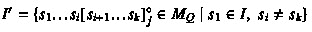
As the paths $\pi _1,\pi _2,\ldots ,\pi _k$ are tracked in a parallel and synchronous way, the states $s_1,s_2,\ldots ,s_k$ of a macrostate have to be pairwise different with a possible exception of states $s_i=s_k$. Formally, we define the set of macrostates built from the set of states Q as

Now we are ready to define a tight automaton $\mathcal {A} ^{\dagger }$ equivalent to $\mathcal {A}$.

Definition 1

Let $\mathcal {A}= (Q, \varSigma , \delta , I, \delta _F)$ be a TBA. We define the TBA $\mathcal {A} ^{\dagger }$ as $\mathcal {A} ^{\dagger }=(Q\cup M_Q,\varSigma ,\delta \cup \delta ',I\cup I',\delta _F\cup \delta _F')$, where

• $\delta '=\delta _1\cup \delta _2\cup \delta _3$ consists of three kinds of transitions,

•  , and

• $\delta _F'=\delta _3$.

The transitions in $\delta _1\cup \delta _2\cup \delta _3$ involve macrostates. They are defined as follows.

These transitions are used to nondeterministically choose the numbers i, j, k and the initial states of $\pi _2,\pi _3,\ldots ,\pi _k$ when reading the last symbol of $minS (u)$. If $minS (u)=\varepsilon$, the nondeterministic choice is done by starting the computation in a macrostate of $I'$.

These transitions simultaneously track the progress on the paths $\pi _1,\pi _2,\ldots ,\pi _k$ including the information whether $\pi _j$ has already passed an accepting transition or not. The condition $s_l\xrightarrow {a}r_l\not \in \delta _F$ for $i<l<j$ enforces that $\pi _j$ is the leftmost path on the loop $\pi _1\pi _2\ldots \pi _k$ containing an accepting transition.

These accepting transitions can enclose a cycle on macrostates if the last state of $\pi _l$ matches the first state of $\pi _{l+1}$ for each $1\le l<k$, the last state of $\pi _k$ matches the first state of $\pi _{i+1}$, and $\pi _j$ has passed an accepting transition in the past or during this step.

Theorem 1

Let $\mathcal {A}= (Q, \varSigma , \delta , I, \delta _F)$ be a TBA. Then $L(\mathcal {A}) = L( \mathcal {A} ^{\dagger })$.

Proof

The inclusion $L(\mathcal {A})\subseteq L( \mathcal {A} ^{\dagger })$ is trivial as each accepting run of $\mathcal {A}$ is also an accepting run of $\mathcal {A} ^{\dagger }$.

We show that $L( \mathcal {A} ^{\dagger })\subseteq L(\mathcal {A})$. Let $\sigma$ be an accepting run of $\mathcal {A} ^{\dagger }$ that involves some macrostates. Note that all macrostates in the run have to use the same numbers i, j, k. We construct an accepting run $\rho$ of $\mathcal {A}$ over the same word as $\sigma$. Intuitively, $\rho$ will consistently use the transitions of some element of the macrostates in $\sigma$, starting with the first element. Each time $\sigma$ uses a transition of $\delta _3$, $\rho$ will switch to the next element and after the k-th element, it will switch back to the $(i+1)$-st element.

First we define an auxiliary function g that determines for each $l\ge 0$ the element of the macrostate in $\sigma$ that will be followed by the transition $\rho _l$.

$$ g(0)=1 \qquad \qquad g(l+1) = {\left\{ \begin{array}{ll} ~g(l) &{} \text {if }\sigma _l\not \in \delta _3\\ ~g(l)+1 &{} \text {if }\sigma _l\in \delta _3\text { and }g(l)<k\\ ~i+1 &{} \text {if }\sigma _l\in \delta _3\text { and }g(l)=k \end{array}\right. } $$

Now we construct $\rho$ as follows.

One can easily check that $\rho$ is a run of $\mathcal {A}$ over the same word as $\sigma$. Further, because $\sigma$ is accepting, it contains infinitely many transitions of $\delta _3$. Hence, there are infinitely many pairs m, l such that $0<m<l$ and

$$g(m-1)\ne j=g(m)=g(m+1)=\ldots =g(l-1)\ne g(l).$$

The definition of g implies that $\sigma _{m-1,l}\in \delta _3.\delta _2^*.\delta _3$, which means that the j-th element of some macrostate in $\sigma _{m,l}$ takes an accepting transition in $\delta _F$. The construction of $\rho$ guarantees that $\rho _{m,l}$ contains the same transition in $\delta _F$. Hence, $\rho$ contains infinitely many accepting transitions and it is therefore accepting.   $\square$

Theorem 2

Let $\mathcal {A}= (Q, \varSigma , \delta , I, \delta _F)$ be a TBA. Then $\mathcal {A} ^{\dagger }$ is tight.

Proof

Lemma 3 implies that for each lasso-shaped word $u\in L(\mathcal {A})$, there exists a minimal run of $\mathcal {A}$ over u. The validity of the statement then follows directly from the properties of minimal runs proven in Lemmata 4 and 5 and from the design of the tightening construction.   $\square$

4.1 State-based tight automata

While our tightening construction produces automata with transition-based acceptance, the previous tightening constructions [13, 23, 24] produce automata with state-based acceptance. Some applications [27] also work with tight state-based automata on the input. Therefore, we present a transformation of a tight TBA to an equivalent BA preserving tightness.

Let $\mathcal {A}= (Q,\varSigma ,\delta ,I,\delta _F)$ be a tight TBA. An equivalent tight BA $\mathcal {B}$ can be constructed as follows. We define the set of accepting states as duplicates of states $q\in Q$ that have some accepting transition starting in q, i.e., $F=\{\overline{q}\mid q\xrightarrow {a}p\in \delta _F\}$. We extend the initial states and the transition relation in such a way that whenever the original automaton can use an accepting transition from a state q, the resulting state-based automaton can reach the corresponding state $\overline{q}$ and use an analogous transition from it. Formally, the tight BA $\mathcal {B}$ equivalent to $\mathcal {A}$ is constructed as $\mathcal {B}=(Q\cup F,\varSigma ,\delta \cup \delta ',I\cup I',F)$, where

• $I' = \{\overline{q} \mid q\in I\}\cap F$ and

• $\delta '=\{p\xrightarrow {a}\overline{q}\mid p\xrightarrow {a}q\in \delta ,~\overline{q}\in F\}\cup \{\overline{p}\xrightarrow {a}\overline{q}\mid p\xrightarrow {a}q\in \delta _F,~\overline{p},\overline{q}\in F\}\cup$

  $\cup \{\overline{p}\xrightarrow {a}q\mid p\xrightarrow {a}q\in \delta _F,~\overline{p}\in F\}$.

Each accepting run $\sigma$ of $\mathcal {B}$ can be transformed to an accepting run $\rho$ of $\mathcal {A}$ over the same word simply by replacing each state $\overline{q}\in F$ by the corresponding state q. Thus we get $L(\mathcal {B})\subseteq L(\mathcal {A})$.

Further, each accepting run $\rho$ of $\mathcal {A}$ can be transformed into an accepting run $\sigma$ of $\mathcal {B}$ over the same word simply by replacing each state q from which an accepting transition is taken with the corresponding state $\overline{q}$. This implies $L(\mathcal {A})\subseteq L(\mathcal {B})$. Moreover, when we apply this transformation to a tight run $\rho$ of $\mathcal {A}$, we obtain a tight run $\sigma$ of $\mathcal {B}$. To sum up, the automata $\mathcal {A}$ and $\mathcal {B}$ are equivalent and if $\mathcal {A}$ is tight, then $\mathcal {B}$ is also tight.

4.2 Upper bound for tightening

Lemma 6

Let $\mathcal {A}$ be a TBA with n states. The number of states in $\mathcal {A} ^{\dagger }$ is at most

$$\begin{aligned} n\,+\,2\cdot \sum _{k=2}^{n}\frac{n!\cdot k\cdot (k+1)}{(n-k)!}~\in ~\mathcal {O}(n!\cdot n^3). \end{aligned}$$

Proof

Let Q be the set of states of $\mathcal {A}$. First we bound the number of macrostates of the form for a fixed i, j, k. There are $\frac{n!}{(n-k)!}\cdot 2$ cases where all states $s_1,s_2,\ldots ,s_k$ are pairwise different and $\frac{n!}{(n-(k-1))!}\cdot 2$ cases where $s_1,s_2,\ldots ,s_{k-1}$ are pairwise different and $s_k=s_i$. The factor 2 comes from ${\star }\in \{{\circ } ,{\bullet }\}$. Altogether, $M_Q$ contains at most $4\cdot \frac{n!}{(n-k)!}$ macrostates for fixed i, j, k. Further, for a fixed $k\ge 2$, there are $\frac{k\cdot (k+1)}{2}$ possible pairs of values of i, j satisfying $0\le i<j\le k$. Altogether, the number of macrostates in $M_Q$ can be bounded by $\sum _{k=2}^{n}4\cdot \frac{n!}{(n-k)!}\cdot \frac{k\cdot (k+1)}{2}= 2\cdot \sum _{k=2}^{n}\frac{n!\cdot k\cdot (k+1)}{(n-k)!}$. When we add the number $n=|Q|$ of the original states, we get the statement.   $\square$

Recall that each BA can be seen as a special case of a TBA. Further, note that the transformation of tight TBA to tight BA presented in Section 4.1 only doubles the state space in the worst case. Hence, we also proved that each BA or TBA with n states can be transformed into an equivalent tight BA with at most $\mathcal {O}(n!\cdot n^3)$ states. This upper bound is tighter (i.e., asymptotically smaller) than the upper bound $2^{\mathcal {O}(n^2)}$ by Ehlers [13] and than the upper bound $\mathcal {O}((\sqrt{2}n)^{2n})$ derived from the Schuppan’s construction [23] as

$$ \lim _{n\rightarrow \infty } \frac{n!\cdot n^3}{2^{n^2}} ~~=~~ \lim _{n\rightarrow \infty } \frac{n!\cdot n^3}{(\sqrt{2}n)^{2n}} ~~=~~ 0. $$

5 Lower bound for tightening

We present a lower bounds for any transformation of a TBA or a BA to an equivalent tight TBA or BA.

Lemma 7

For each $n>0$, there is a TBA $\mathcal {A}$ with $n+1$ states and an equivalent BA $\mathcal {A}'$ with 2n+1 states such that for every equivalent tight TBA $\mathcal {B}$ with the set of states Q it holds that

$$\begin{aligned} |Q|~\ge ~\sum _{k=1}^{n}\frac{n!}{(n-k)!}. \end{aligned}$$

Proof

Let us fix some $n>0$. We construct the TBA $\mathcal {A}$ with $n+1$ states gradually as follows. The automaton uses states $\{q_0\}\cup Q'$ where $q_0$ is the only initial state and $Q'$ contains another n states. The construction works with nonempty sequences of pairwise different states from $Q'$. For each , we add fresh symbols a, b to the alphabet of $\mathcal {A}$ and the transitions depicted in Figure 4 to the transition relation of $\mathcal {A}$. The automaton accepts $a.b^\omega$ with these transitions. The constructed automaton for $n=2$ is in Figure 5. The equivalent BA $\mathcal {A}'$ is constructed from $\mathcal {A}$ by the transformation given in Section 4.1.

Fig. 4.

The construction of the transitions for a given .

Fig. 5.

The automaton $\mathcal {A}$ for $n=2$. The construction considers 4 sequences and each sequence induced transitions that accept the following words: [s] relates to the word $a_0.b_0^\omega$, [rs] to $a_1.b_1^\omega$, [r] to $a_2.b_2^\omega$, and [sr] to $a_3.b_3^\omega$.

Now we assume that $\mathcal {B}=(Q,\varSigma ,\delta ,I,\delta _F)$ is a tight TBA equivalent to $\mathcal {A}$. Each induces the acceptance of a new word $a.b^\omega \in L(\mathcal {A})=L(\mathcal {B})$. As $\mathcal {B}$ is tight and $| minSL (a.b^\omega )|=2$, there have to be transitions $p\xrightarrow {a}q\in \delta$ and $q\xrightarrow {b}q\in \delta _F$ for some states $p\in I$ and $q\in Q$. We prove by contradiction that the state q has to be different for each .

Let us assume that and are different sequences inducing the acceptance of $a.b^\omega$ and $a'.b'^\omega$, respectively, and $\mathcal {B}$ accepts these two words using transitions $p\xrightarrow {a}q,p'\xrightarrow {a'}q\in \delta$ and $q\xrightarrow {b}q,q\xrightarrow {b'}q\in \delta _F$. The situation is depicted in Figure 6.

Fig. 6.

Illustration of the assumption. States p and $p'$ does not have to be different.

We distinguish two cases.

• 1. $\{s_{1},\dots ,s_k\}\ne \{r_{1},\dots ,r_{k'}\}$:  Without loss of generality, we assume that $r_j\not \in \{s_{1},\dots ,s_k\}$. As $\mathcal {B}$ accepts all words in $\{a'\}.\{b,b'\}^\omega$, it also accepts the word $a'.b'^{j-1}.b^\omega$. However, this word is not in $L(\mathcal {A})$ as $\mathcal {A}$ is deterministic and after reading $a'.b'^{j-1}$ it gets to state $r_j$ which has no transition over b since since $r_j\not \in \{s_1,\dots ,s_k\}$. Hence, $L(\mathcal {B}) \ne L(\mathcal {A})$ and this is a contradiction with our assumptions.

• 2. $\{s_1,\dots ,s_k\}=\{r_1,\dots ,r_{k'}\}$:  As states in each sequence are not repeating, we get $k=k'$. We use the fact that the only accepting transitions over b and $b'$ in $\mathcal {A}$ are those from $s_1$ and $r_1$, respectively. We distinguish two subcases:

  • (a) $s_1=r_1$:  Let j be the smallest number such that $s_j\ne r_j$. As the sets of states are equal, there exist $j < m,m' \le k$, such that $s_m = r_j$ and $r_{m'} = s_j$. Consider the run $\tau .\pi ^\omega$ of $\mathcal {A}$, where

    

    As $\pi$ contains no accepting transition, the run is not accepting. Since $\mathcal {A}$ is deterministic, it is the only run of $\mathcal {A}$ over $a.b^{j-1}.(b^{m-j}b'^{m'-j})^{\omega }$. As the word is accepted by $\mathcal {B}$, we get a contradiction with $L(\mathcal {A})=L(\mathcal {B})$.

  • (b) $s_1\ne r_1$:  Since the sequences contain the same states, there are some $1 \le m,l \le k$ such that $s_1\xrightarrow {b'^{m}}r_1$ and $r_1\xrightarrow {b^l}s_1$. Consider the run $\tau .\pi ^\omega$ of $\mathcal {A}$, where

    $$ \tau =q_0\xrightarrow {a}s_1\qquad \text { and }\qquad \pi =s_1\xrightarrow {b'^m}r_1\xrightarrow {b^l}s_1. $$

    The run is not accepting as the only accepting transitions over b or $b'$ starting in $s_1$ and $r_1$, respectively, are never taken. Since $\mathcal {A}$ is deterministic, it is the only run of $\mathcal {A}$ over $a.(b'^{m}b^{l})^{\omega }$. As the word is accepted by $\mathcal {B}$, we get a contradiction with $L(\mathcal {A})=L(\mathcal {B})$.

To sum up, we proved that every tight TBA $\mathcal {B}$ satisfying $L(\mathcal {B}) = L(\mathcal {A})$ must have at least one state for every nonempty sequence . This directly implies that the number of its states is at least $\sum _{k=1}^{n}\frac{n!}{(n-k)!}$.    $\square$

The previous lemma says that for each $n\ge 2$, there exists a TBA with n states such that the smallest equivalent tight TBA (and thus also the smallest equivalent tight BA) has at least $\sum _{k=1}^{n-1}\frac{(n-1)!}{(n-1-k)!}$ states. This function is clearly in $\varOmega ((n-1)!)$ as

$$ \lim _{n\rightarrow \infty } \frac{\sum _{k=1}^{n-1}\frac{(n-1)!}{(n-1-k)!}}{(n-1)!} ~~=~~ \lim _{n\rightarrow \infty } \sum _{k=1}^{n-1}\frac{1}{(n-1-k)!} ~~=~~ \sum _{k=0}^{\infty }\frac{1}{k!} ~~=~~ e. $$

Note that the difference between the upper bound $\mathcal {O}(n!\cdot n^3)=\mathcal {O}((n-1)!\cdot n^4)$ given in Lemma 6 and the lower bound $\varOmega ((n-1)!)$ is only the factor $n^4$.

Analogous arguments lead to the statement that for each odd $n\ge 3$ there exists a BA with n states such that the smallest equivalent tight TBA (and thus also the smallest equivalent tight BA) has at least $\varOmega (\frac{n-1}{2}!)$ states. This lower bound is above the previously known lower bound $2^{\varOmega (n)}$ as for each c it holds

$$ \lim _{n\rightarrow \infty } \frac{2^{cn}}{\frac{n-1}{2}!} ~~=~~ 0. $$

6 Postprocessing of tight automata

This section shows that a standard automata reduction technique called quotienting [8] preserves tightness. Hence, it can be applied to reduce tight automata before they are further processed.

Consider an automaton with the set of states Q. A preorder ${\sqsubseteq }\subseteq Q\times Q$ is a reflexive and transitive relation. Every preorder defines an induced equivalence ${\approx } = {\sqsubseteq }\cap {\sqsupseteq }$. Given a state q, we denote by [q] the equivalence class of q with respect to a fixed equivalence $\approx$. Furthermore, for every $P\subseteq Q$, by [P] we denote the set $[P] = \{[q]\mid q\in P\}$ of all equivalence classes of states in P.

Given a TBA $\mathcal {A}= (Q, \varSigma , \delta , I, \delta _F)$ and a preorder $\sqsubseteq$ on Q with its induced equivalence $\approx$, the quotient of $\mathcal {A}$ is the TBA $\mathcal {A}/{\sqsubseteq } = ([Q], \varSigma , \delta ', [I], \delta _F')$, where $\delta '=\{[q]\xrightarrow {a}[p]\mid q\xrightarrow {a}p\in \delta \}$ and $\delta _F'=\{[q]\xrightarrow {a}[p]\mid q\xrightarrow {a}p\in \delta _F\}$.

A preorder $\sqsubseteq$ is good for quotienting (GFQ) [8] if $L(\mathcal {A}) = L( \mathcal {A}/{\sqsubseteq })$ for each TBA $\mathcal {A}$. There exist many preorders that are GFQ, for example various kinds of forward or backward simulation or trace inclusion. For their definition and more information about automata reduction techniques we refer to the comprehensive paper by Clemente and Mayr [8].

Lemma 8

Let $\mathcal {A}$ be a tight TBA and let $\sqsubseteq$ be a GFQ preorder. The automaton $\mathcal {A}/{\sqsubseteq }$ is tight and $L(\mathcal {A}) = L( \mathcal {A}/{\sqsubseteq })$.

Proof

The language equivalence trivially follows from the definition of GFQ. Let us consider an arbitrary lasso-shaped word $u\in L(\mathcal {A})$. As $\mathcal {A}$ is tight, it has an accepting run $\rho =\tau .\pi ^\omega$ where $\tau$ has the form $q_0\xrightarrow { minS (u)}l$ and $\pi$ has the form $l\xrightarrow { minL (u)}l$. The definition of quotient implies that for each accepting run of $\mathcal {A}$ there exists an accepting run over the same word through the corresponding equivalence classes in $\mathcal {A}/{\sqsubseteq }$. Hence, $\mathcal {A}/{\sqsubseteq }$ has an accepting run $\rho '=\tau '.\pi '^{\omega }$ where $\tau '$ has the form $[q_0]\xrightarrow { minS (u)}[l]$ and $\pi '$ has the form $[l]\xrightarrow { minL (u)}[l]$. It is easy to see that $| minSL (\rho ')| \le | minSL (\rho )|$ and thus $\rho '$ is tight. Therefore, the automaton $\mathcal {A}/{\sqsubseteq }$ is tight.   $\square$

7 Implementation

We have implemented our tightening construction in a tool called Tightener. The tool is written in Python 3.8.15 and it is built upon the library for LTL and $\omega$-automata called Spot [10] in version 2.11.4. Spot provides state-of-the-art LTL to automata translations, efficient transformations of arbitrary automata in the HOA format [2] to equivalent TBA, and some automata reduction techniques, in particular direct simulation [8] that is good for quotienting.

Tightener can take as an input either an LTL formula or an automaton in the HOA format. The input is internally translated into an equivalent TBA using the functionality provided by the Spot library. The TBA is then transformed into a tight TBA or tight state-based BA using the construction presented in this paper. The tight automaton is then optionally reduced using Spot’s function reduce_direct_sim which performs quotienting by direct simulation. The resulting tight automaton is encoded in DOT or in the HOA format.

Tightener is available in an artifact at Zenodo¹ and at the project repository² under the GNU Public License, version 3[1]. The tool can be run in the directory Tightener_project using the command python Tightener.py [flags] "input". The tool supports the following flags.

• -h or –help describes the basic usage of the tool.

• -f or –formula says that the "input" is an LTL formula (e.g., "Fp1 | Fp2") on the command line. Tightener uses the same syntax for LTL formulas as Spot, see https://spot.lre.epita.fr/ioltl.html.

• -F or –file says that the "input" is a path to a text file containing an LTL formula in the format mentioned above.

• -a or –HOA says that the "input" is a path to a file containing an automaton in the HOA format.

• -s or –sbacc asks to produce a state-based tight automaton. The tool produces tight TBA by default.

• -r or –reduces applies reductions preserving tightness before the tight automaton is returned. These reductions are not applied by default.

• -o or –outputHOA outputs the tight automaton in the HOA format. By default, the tool returns a tight automaton in DOT format, which can be easily visualized, for example at https://dreampuf.github.io/GraphvizOnline/. Note that the DOT format does not support multiple initial states. Hence, if the returned automaton has multiple initial states, one of them is marked as initial and the others are identified by an auxiliary incoming edge labeled with init.

8 Experimental results

We compare Tightener against the translation of LTL to state-based generalized Büchi automata introduced by Clarke, Grumberg, and Hamaguchi [6] and called CGH. Schuppan and Biere [24] proved that the automata produced by CGH are tight. As far as we know, this is the only existing implementation besides Tightener that produces tight automata. Still, the comparison is not entirely fair as Tightener and CGH have different input and different output: Tightener can transform any LTL formula or automaton in the HOA format to tight TBA or BA, CGH accepts only an LTL formula and produces a tight GBA. BA can be seen as a special case of both TBA and GBA, but the opposite does not hold. We provided a transformation of tight TBA into equivalent tight BA in Section 4.1. Each GBA can be transformed into an equivalent BA (this so-called degeneralization process has been recently significantly improved [3]), but the transformation increases the number of states and it does not guarantee to preserve tightness. We therefore compare the size of tight GBA produced by CGH against the size of tight TBA and tight BA produced by Tightener.

Since CGH produces tight GBA in symbolic representation, we implemented a process that enumerates automata states from this symbolic representation and uses the SMT solver Z3 [9] to prune unreachable and contradictory states. In the end, we count the number of reachable states. This implementation can be also found in our repository in script Tightener_project/CGH_implementation.py.

Table 2. We compare the tight TBA and BA produced by Tightener against the GBA constructed by CGH. For both datasets, the table shows the number [#] and the percentage [%] of cases where the corresponding tool provided a tight automaton with fewer states than the other tool. Columns avg. size represent the average number of states of the automata constructed by the corresponding tool. Columns TO indicate the number of timeouts. Cases where Tightener timed out are counted in the CGH winning columns, but these cases are excluded from the computation of average size.

We compare CGH and Tightener on two sets of LTL formulas. The first dataset contains 642 formulas produced by random formulas generator rand_ltl of Spot’s. These formulas are stored in file ltlDataSet_random.txt in our repository. The second dataset consists of 219 formulas taken from literature[4, 11, 14, 16,17,18, 21, 25, 26]. We obtained these formulas from the tool gen_ltl of Spot and they are stored in file ltlDataSet_pattern.txt in our repository.

We ran the experiments on a machine with an AMD Ryzen 7 PRO 4750U processor and 32 GB of RAM. We set 15 minutes timeout limit per task with no explicit memory limit.

Each formula has been translated by Tightener to a tight TBA and to a tight BA with reduction switched on in both cases, and by CGH to a tight GBA. Table 2 summarizes the cummulative results for the two datasets. One can see that Tightener constructs smaller automata in substantially more cases than CGH in both considered datasets and with both settings. However, Tightener run out of time in some cases.

The scatter plots in Figure 7 compare the number of states of the tight automata constructed by CGH and Tightener for individual LTL formulas in each dataset. Since some of the produced automata are rather large, we use logarithmic scale in all of the scatter plots. The graphs clearly show that Tightener often produces dramatically smaller tight automata than CGH.

Fig. 7.

The comparison of the number of states of the tight automata produced by Tightener and CGH for individual LTL formulas of each dataset. In the top row, Tightener produces tight TBA. In the bottom row, it produces tight BA. CGH always produces GBA. The red crosses display the cases where Tightener reaches a time limit.

8.1 Experiments on formulas for robot action planning

Tumova et al. [27] introduced a technique that generates control strategies for a robot planning problem. They represent the strategies as lasso-shaped words, where alphabet is a set of locations and possible actions in the respective location. Their approach takes advantage of tight BA to obtain the strategies with the shortest length of the stem and the loop.

The paper contains three LTL formulas representing meaningful properties. Table 3 compares the sizes of tight BA obtained from Tightener and tight GBA from CGH on these formulas. For two of the formulas, Tightener constructed dramatically smaller automaton than CGH. On the third formula, Tightener produced a tight BA with 2 states while CGH ran out of time.

Table 3. Sizes of tight automata constructed from LTL formulas taken from the study of Tumova et al. [27]. TO indicates a timeout.

9 Conclusions

In this paper, we presented a new approach for converting TBA or BA to tight TBA or BA. We proved that the asymptotical rise of the state space is $O(n!\cdot n^3)$, which is the smallest upper bound so far reached. Further, we proved the highest lower bounds on the rise of the state-space of tight automata so far reached, making the theoretical construction of tight automata significantly tighter. We also showed that the good-for-quotienting simulations can be used to reduce automata while preserving tightness.

Our tool Tightener opens new ways to construct tight automata as it is the first tool that can create tight automata from arbitrary automata in the HOA format or from LTL formulas. We compared Tightener against the LTL to tight automata translation CGH on two datasets of LTL formulas. Experiments show that Tightener constructs smaller tight automata in substantially more cases. Moreover, we compared the two tools on three formulas for which a tight automaton was explicitly desired before. In all three cases, Tightener provided a dramatically better result.

Funding Statement. Until June 2023, M. Jankola was supported by the European Union’s Horizon Europe program under the grant agreement No. 101087529 and since July 2023 by the Deutsche Forschungsgemeinschaft (DFG) – 378803395 (ConVeY). J. Strejček was supported by the Czech Science Foundation grant GA23-06506S.

References

GNU general public license, version 3. http://www.gnu.org/licenses/gpl.html, June 2007. Last retrieved 2020-01-01
Tomáš Babiak, František Blahoudek, Alexandre Duret-Lutz, Joachim Klein, Jan Křetínský, David Müller, David Parker, and Jan Strejček. The Hanoi omega-automata format. In Daniel Kroening and Corina S. Pasareanu, editors, Computer Aided Verification - 27th International Conference, CAV 2015, San Francisco, CA, USA, July 18-24, 2015, Proceedings, Part I, volume 9206 of Lecture Notes in Computer Science, pages 479–486. Springer, 2015. See also http://adl.github.io/hoaf/
Antonio Casares, Alexandre Duret-Lutz, Klara J. Meyer, Florian Renkin, and Salomon Sickert. Practical applications of the alternating cycle decomposition. In Dana Fisman and Grigore Rosu, editors, Tools and Algorithms for the Construction and Analysis of Systems - 28th International Conference, TACAS 2022, Held as Part of the European Joint Conferences on Theory and Practice of Software, ETAPS 2022, Munich, Germany, April 2-7, 2022, Proceedings, Part II, volume 13244 of Lecture Notes in Computer Science, pages 99–117. Springer, 2022
Jacek Cichoń, Adam Czubak, and Andrzej Jasiński. Minimal Büchi automata for certain classes of LTL formulas. In Proceedings of the Fourth International Conference on Dependability of Computer Systems (DEPCOS’09), pages 17–24. IEEE Computer Society, 2009
Alessandro Cimatti, Edmund Clarke, Enrico Giunchuglia, Fausto Giunchiglia, Marco Pistore, Macro Roveri, Roberto Sebastiani, and Armando Tacchella. Nusmv 2: An opensource tool for symbolic model checking. In E. Brinksma and K. Guldstrand Larsen, editors, Proceedings of the 14th International Conference on Computer Aided Verification (CAV’02), volume 2404 of Lecture Notes in Computer Science, pages 359–364, Copenhagen, Denmark, July 2002. Springer-Verlag
Edmund M. Clarke, Orna Grumberg, and Kiyoharu Hamaguchi. Another look at LTL model checking. In David L. Dill, editor, Computer Aided Verification, 6th International Conference, CAV ’94, Stanford, California, USA, June 21-23, 1994, Proceedings, volume 818 of Lecture Notes in Computer Science, pages 415–427. Springer, 1994
Edmund M. Clarke, Orna Grumberg, Kenneth L. McMillan, and Xudong Zhao. Efficient generation of counterexamples and witness in symbolic model checking. In Proceedings of the 32nd ACM/IEEE Design Automation Conference (DAC’95), pages 427–432, San Francisco, California, USA, June 1995. ACM Press
Lorenzo Clemente and Richard Mayr. Efficient reduction of nondeterministic automata with application to language inclusion testing. Log. Methods Comput. Sci., 15(1), 2019
Leonardo Mendonça de Moura and Nikolaj S. Bjørner. Z3: an efficient SMT solver. In C. R. Ramakrishnan and Jakob Rehof, editors, Tools and Algorithms for the Construction and Analysis of Systems, 14th International Conference, TACAS 2008, Held as Part of the Joint European Conferences on Theory and Practice of Software, ETAPS 2008, Budapest, Hungary, March 29-April 6, 2008. Proceedings, volume 4963 of Lecture Notes in Computer Science, pages 337–340. Springer, 2008
Alexandre Duret-Lutz, Etienne Renault, Maximilien Colange, Florian Renkin, Alexandre Gbaguidi Aisse, Philipp Schlehuber-Caissier, Thomas Medioni, Antoine Martin, Jérôme Dubois, Clément Gillard, and Henrich Lauko. From Spot 2.0 to Spot 2.10: What’s new? In Sharon Shoham and Yakir Vizel, editors, Computer Aided Verification - 34th International Conference, CAV 2022, Haifa, Israel, August 7-10, 2022, Proceedings, Part II, volume 13372 of Lecture Notes in Computer Science, pages 174–187. Springer, 2022
Matthew B. Dwyer, George S. Avrunin, and James C. Corbett. Property specification patterns for finite-state verification. In Mark Ardis, editor, Proceedings of the 2nd Workshop on Formal Methods in Software Practice (FMSP’98), pages 7–15, New York, March 1998. ACM Press
Rüdiger Ehlers. Short witnesses and accepting lassos in \(\omega \)-automata. In Adrian-Horia Dediu, Henning Fernau, and Carlos Martín-Vide, editors, Language and Automata Theory and Applications, 4th International Conference, LATA 2010, Trier, Germany, May 24-28, 2010. Proceedings, volume 6031 of Lecture Notes in Computer Science, pages 261–272. Springer, 2010
Rüdiger Ehlers. How hard is finding shortest counter-example lassos in model checking? In Maurice H. ter Beek, Annabelle McIver, and José N. Oliveira, editors, Formal Methods - The Next 30 Years - Third World Congress, FM 2019, Porto, Portugal, October 7-11, 2019, Proceedings, volume 11800 of Lecture Notes in Computer Science, pages 245–261. Springer, 2019
Kousha Etessami and Gerard J. Holzmann. Optimizing Büchi automata. In C. Palamidessi, editor, Proceedings of the 11th International Conference on Concurrency Theory (Concur’00), volume 1877 of Lecture Notes in Computer Science, pages 153–167, Pennsylvania, USA, 2000. Springer-Verlag
Paul Gastin, Pierre Moro, and Marc Zeitoun. Minimization of counterexamples in SPIN. In S. Graf and L. Mounier, editors, Proceedings of the 11th International SPIN Workshop on Model Checking of Software (SPIN’04), volume 2989 of Lecture Notes in Computer Science, pages 92–108, April 2004
Paul Gastin and Denis Oddoux. Fast LTL to Büchi automata translation. In G. Berry, H. Comon, and A. Finkel, editors, Proceedings of the 13th International Conference on Computer Aided Verification (CAV’01), volume 2102 of Lecture Notes in Computer Science, pages 53–65, Paris, France, 2001. Springer-Verlag
Jaco Geldenhuys and Henri Hansen. Larger automata and less work for LTL model checking. In Proceedings of the 13th International SPIN Workshop (SPIN’06), volume 3925 of Lecture Notes in Computer Science, pages 53–70. Springer, 2006
Jan Holeček, Tomáš Kratochvíla, Vojtěch Řehák, David Šafránek, and Pavel Šimeček. Verification results in Liberouter project. Technical Report 03/2004, CESNET Technical Report, 2004
Orna Kupferman and Sarai Sheinvald-Faragy. Finding shortest witnesses to the nonemptiness of automata on infinite words. In Christel Baier and Holger Hermanns, editors, CONCUR 2006 - Concurrency Theory, 17th International Conference, CONCUR 2006, Bonn, Germany, August 27-30, 2006, Proceedings, volume 4137 of Lecture Notes in Computer Science, pages 492–508. Springer, 2006
Orna Kupferman and Moshe Y. Vardi. Model checking of safety properties. In N. Halbwachs and D. Peled, editors, Proceedinfs of the 11th International Conference on Computer Aided Verification (CAV’99), volume 1633 of Lecture Notes in Computer Science, pages 172–183. Springer-Verlag, 1999
Radek Pelánek. BEEM: benchmarks for explicit model checkers. In Proceedings of the 14th international SPIN conference on Model checking software, Lecture Notes in Computer Science, pages 263–267. Springer-Verlag, 2007
Kavita Ravi, Roderick Bloem, and Fabio Somenzi. A comparative study of symbolic algorithms for the computation of fair cycles. In J. W. O’Leary M. D. Aagaard, editor, Proceedings of the 4th International Conference on Formal Methods in Computer Aided Design (FMCAD’00), volume 2517 of Lecture Notes in Computer Science, pages 143–160. Springer-Verlag, 2000
Viktor Schuppan. Liveness checking as safety checking to find shortest counterexamples to linear time properties. PhD thesis, ETH Zurich, 2006
Viktor Schuppan and Armin Biere. Shortest counterexamples for symbolic model checking of LTL with past. In Nicolas Halbwachs and Lenore D. Zuck, editors, Tools and Algorithms for the Construction and Analysis of Systems, 11th International Conference, TACAS 2005, Held as Part of the Joint European Conferences on Theory and Practice of Software, ETAPS 2005, Edinburgh, UK, April 4-8, 2005, Proceedings, volume 3440 of Lecture Notes in Computer Science, pages 493–509. Springer, 2005
Fabio Somenzi and Roderick Bloem. Efficient Büchi automata for LTL formulæ. In Proceedings of the 12th International Conference on Computer Aided Verification (CAV’00), volume 1855 of Lecture Notes in Computer Science, pages 247–263, Chicago, Illinois, USA, 2000. Springer-Verlag
Deian Tabakov and Moshe Y. Vardi. Optimized temporal monitors for SystemC. In Proceedings of the 1st International Conference on Runtime Verification (RV’10), volume 6418 of Lecture Notes in Computer Science, pages 436–451. Springer, November 2010
Jana Tumova, Alejandro Marzinotto, Dimos V. Dimarogonas, and Danica Kragic. Maximally satisfying LTL action planning. In 2014 IEEE/RSJ International Conference on Intelligent Robots and Systems, Chicago, IL, USA, September 14-18, 2014, pages 1503–1510. IEEE, 2014
Author information
Authors and Affiliations
Corresponding author
Editor information
Editors and Affiliations
Rights and permissions
Open Access This chapter is licensed under the terms of the Creative Commons Attribution 4.0 International License (http://creativecommons.org/licenses/by/4.0/), which permits use, sharing, adaptation, distribution and reproduction in any medium or format, as long as you give appropriate credit to the original author(s) and the source, provide a link to the Creative Commons license and indicate if changes were made.
The images or other third party material in this chapter are included in the chapter's Creative Commons license, unless indicated otherwise in a credit line to the material. If material is not included in the chapter's Creative Commons license and your intended use is not permitted by statutory regulation or exceeds the permitted use, you will need to obtain permission directly from the copyright holder.
Copyright information
© 2024 The Author(s)
About this paper
Cite this paper
Jankola, M., Strejček, J. (2024). Tighter Construction of Tight Büchi Automata. In: Kobayashi, N., Worrell, J. (eds) Foundations of Software Science and Computation Structures. FoSSaCS 2024. Lecture Notes in Computer Science, vol 14574. Springer, Cham. https://doi.org/10.1007/978-3-031-57228-9_12
Download citation
DOI: https://doi.org/10.1007/978-3-031-57228-9_12
Published:
Publisher Name: Springer, Cham
Print ISBN: 978-3-031-57227-2
Online ISBN: 978-3-031-57228-9
eBook Packages: Computer ScienceComputer Science (R0)