Calibration Curves in Quantitative Ligand Binding Assays: Recommendations and Best Practices for Preparation, Design, and Editing of Calibration Curves

Abstract

The accuracy of reported sample results is contingent upon the quality of the assay calibration curve, and as such, calibration curves are critical components of ligand binding and other quantitative methods. Regulatory guidance and lead publications have defined many of the requirements for calibration curves which encompass design, acceptance criteria, and selection of a regression model. However, other important aspects such as preparation and editing guidelines have not been addressed by health authorities. The goal of this publication is to answer many of the commonly asked questions and to present a consensus and the shared views of members of the ligand binding assay (LBA) community on topics related to calibration curves with focus on providing recommendations for the preparation and editing of calibration curves.

Introduction

Calibration curves illustrate the relationship between the detected response variable and the concentration of a reference standard that is presumed to be representative of the analyte of interest in a test sample. They are used to estimate the unknown concentration of the analyte of interest in a test sample by dose interpolation. Calibration curves are prepared by spiking the target analyte into a matrix that has been judged to be representative of the test sample matrix. The instrument read-out values for unknown samples and quality controls (QCs) are subsequently used to interpolate their concentrations from the calibration (or standard) curve. Three factors should be given consideration for optimal fitting of non-linear calibration curves. These include fitting the mean concentration response relationship, use of an appropriate weighting to account for the known heteroscedasticity (non-constant response-error relationship) in non-linear dose response curves, and a suitable curve fitting algorithm to estimate the curve fit parameters.

The accuracy of sample quantitation depends on the robustness and reproducibility of the assay calibration curve, which is in turn dependent upon the performance of the reference material and other assay components. Performance characteristics of ligand binding assay (LBA) components which include but are not limited to the solid or immobilized surfaces such as microtiter plates and the capture and detection antibodies should be thoroughly evaluated in the method development phase, and appropriate plans should be put in place to monitor lot to lot reagent consistency. The general requirements for the design of calibration curves, the acceptance criteria for individual calibrators, and the guidelines for the selection of an appropriate regression model have been defined in regulatory guidance documents and lead publications by subject matter experts (1,2,3,4,5,6,7,8,9,10,11,12,13,14,15,16,17). Compliance with these guidelines and adherence to the published requirements would enhance reproducibility of a calibration curve across runs and across studies. Other aspects of calibration curves including editing specifications and preparation guidelines have not been established or adequately addressed. It is ultimately the responsibility of each bioanalytical laboratory to define the criteria for the design, preparation, acceptance, and editing of LBA calibration curves in their standard operating procedures (SOPs). This publication aims to present a collective view from members of the LBA community to fill in gaps by providing recommendations and best practices for the preparation of calibration curves as well as for the treatment of calibrator data points. Although the content of this publication may be applicable to subsets of biomarker assays, its focus remains on calibration curves for quantitative pharmacokinetic (PK) LBAs. All other assay types are outside the scope of this paper.

Calibration Curves in Quantitative Analysis

Non-Linear Nature of Ligand Binding Assay Calibration Curves

There are key differences between calibration curves in LBAs and in chromatographic assays. In LBAs, the instrument response may be directly or inversely related to the analyte concentration depending on the non-competitive or competitive format of the assay. Irrespective of the format, the use of a semi-log scale translates the curve into a sigmodal “S-shaped” relationship between the response and the concentration of the analyte. This is in contrast to the chromatographic assays where response is typically a linear function of the concentration, and the two are proportional over most of the calibration curve range. For chromatographic methods, loss of linearity is an indication that the assay has reached its limits of the detection. LBAs rely upon the interaction of the analyte with a binding agent such as an antibody or a receptor component; this is in contrast to traditional chromatographic assays in which detection of the target analyte is independent of its binding to a macromolecule. The dynamic equilibrium nature of protein-protein interaction leads to a non-linear response in LBAs. Furthermore, since performance of LBAs heavily depends upon the performance of their constituent biological reagents, these assays typically manifest greater variability. The non-linear nature of an LBA curve limits the concentration-response correlation at the upper and lower ends of the curve, resulting in plateaus and therefore an S-shaped curve. Quantitation from the asymptote (upper and lower plateaus) of the calibration curve would result in poor precision and accuracy. These characteristics ultimately narrow the validated quantitative range of LBAs and render the selection of an appropriate non-linear data fitting algorithm all the more important.

Performance and Validation Requirements for Non-Linear Regression Software

There is a wide range of commercial software available to perform non-linear regression for LBAs. Most instrument manufacturers provide a non-linear regression software that is compatible with the equipment. Depending on which better meets their needs and requirements, laboratories may alternatively choose to install a stand-alone software or use their laboratory information management system (LIMS) for regression purposes. There are performance requirements for the software. The software used for LBA calibration curves should have the capability to

• Perform four and five parameter logistic (4 PL and 5 PL) regressions

• Allow for application of various weighting factors

• Calculate %bias

• Determine %CV

• Possess the capability to plot concentration versus %bias for each model with various weighting factors and the response curve

• Allow for editing of the curve and repeat regression after editing

• Be compatible with standard computer equipment, infrastructure, networks, and data processing procedures

• Be compatible with standard or custom system interfaces

• Allow for data acquisition, analysis, and reporting

• Allow for data upload to LIMS

• Include an audit trail feature

• Include an edit lock feature

• Allow for creation of custom immunoassay templates to incorporate the acceptance criteria of the validated method

Software validation is the responsibility of the end user. Additional recommendations and the general requirement for software validation have been provided in Appendix 2.

Calibration Curve Minimum Requirements

Comparison of Requirements from Various Regulatory Agencies

The minimum requirements for calibration standard curves have been established in a number of bioanalytical guidance or in the bioanalytical subsections of regulatory documents. At the same time, several bioanalytical guidance from around the world are still in the draft stage. Guidance documents are generally aligned with regard to the requirements and performance expectations of the LBA curves. Table I summarizes the calibration curve requirements from the US Food and Drug Administration (FDA), European Medicines Agency (EMA), the Japanese Ministry of Health, Labor and Welfare (MHLW), and the Brazilian Sanitary Surveillance Agency (ANVISA) (9,10,11,12,13,14). The FDA and EMA guidance are the lead regulatory documents for the vast majority of bioanalytical laboratories; individual groups should assess their regulatory requirements based on the agency they intend to submit to.

Table I Comparison of Regulatory Agency Requirements for Ligand Binding Assay Calibration Curves

Preparation of Calibrator Standards

Calibrator standards are generated by adding known concentrations of the reference standard into a qualified batch of matrix identical to or consistent with the study matrix. The concentration-response relationship of these calibrator standards establishes the calibration curve of the assay. In studies involving co-administration of multiple drugs, one calibration curve is required per analyte present in the study sample. Preparation of calibrators must be independent of assay QCs (6,11) to prevent the spread or magnification of potential spiking errors. This means that calibrators and QCs may not be prepared from the same intermediate stock of the reference standard. Calibrators may be prepared by serially diluting a primary or intermediate stock of the reference material. It is not required to spike calibrators individually at each level although such practice would add another level of control and allow for monitoring of the spiking accuracy. Irrespective of the composition of the intermediate stocks of the reference standard, calibrators should contain a minimum of 95% study matrix.

Surrogate Matrix

The expectation for LBAs is that where possible, every effort is made to prepare the standard calibrators in a biological matrix which matches the study matrix with respect to species, composition, and matrix pre-processing (4,5,11). For example, if study samples are unfiltered serum, then the calibrator matrix pool must also be prepared from unfiltered serum from the same species. A point to consider is that often the study population has a disease condition, whereas the calibrator matrix is from healthy subjects. Preparation of calibrators in depleted or in surrogate matrix may be justified provided that no other strategy to quantify the analyte exists; for example, when the study uses a matrix that is rare or difficult to obtain, when a therapeutic has an endogenous counterpart, or in the case of biomarker assays. In these situations, the bioanalytical method should be validated using study matrix QCs and study matrix selectivity samples to be evaluated against a calibration curve prepared in the surrogate matrix (4). Additional tests to demonstrate comparability between the dilution curves of the surrogate versus study matrices are also recommended. A commonly accepted method is to test the equivalence of the lower and upper asymptotes, growth rates, and in the case of 5 PL curves, the asymmetry factors. Implementation of parallelism tests has been presented by Yang et al. and Sondag et al. (18,19). Acceptance criteria for these equivalence tests have not been published, while efforts in that direction have been ongoing and presented at scientific meetings (20). Figure 1 provides example of a calibration curve prepared in human plasma but also one that is prepared in a buffer surrogate matrix and is a representation of two parallel curves.

Fig. 1

Representation of parallel plasma and surrogate matrix calibration curves. Instrument response in optical density (OD) is plotted on the y-axis against calibrator concentration in nanograms per milliliter on the x-axis

Use of MRD-Diluted Matrix

Calibrators may be prepared in 100% or minimum required dilution (MRD) diluted matrix. Examples of methods using MRD diluted matrix include but are not limited to methods for rare matrices or those performed on automated platforms where use of 100% matrix could become problematic due to limited availability or due to matrix viscosity. The decision whether calibrators are prepared in 100% or MRD diluted matrix should be based on the assay performance during method development. Specifically, appropriate assessments should be conducted to ensure that calibrator and QC recoveries are within the expected range (e.g., ± 20%) of the nominal value. When prepared in 100% matrix, calibrators will require the same MRD dilution as that applied to assay QCs and study samples. The back-calculated concentrations of unknown samples should be reported as the concentration in 100% matrix.

Qualified Matrix Pool

The selection process for a qualified matrix pool (QMP) for bioanalytical applications is critical. It is recommended to qualify and store sufficient volumes of the matrix pool to last through method development, validation, and at least the first in-study bioanalysis. It is also recommended that the QMP be stored under the same conditions as those set for assay QCs and study samples. For example, if samples are stored at less than or equal to − 65°C, the QMP should also be stored in that temperature range. During method development, individual matrix samples or individual matrix pools may be screened, selected, and consolidated to generate a QMP. Individual commercial pooled lots of the matrix may also be applied. QMP screening should include evaluation of assay signal generated by the unfortified as well as the analyte-fortified matrix samples. For screening purposes, individual samples may, for example, be spiked at the LLOQ level. Matrix samples with high background or suboptimal spiked recoveries should be excluded from the QMP. Example acceptance for matrix samples may be that a minimum of 80% of all spiked individual matrix samples meet analytical recovery acceptance criterion of 80 to 120% of the nominal concentration based on a calibration curve prepared with the QMP. The QMP should be representative of the study population and prepared by pooling only the individual matrix samples which meet the targeted acceptance criteria.

Fresh Versus Frozen Calibrators

LBA calibrators may be freshly prepared or frozen. Some laboratories use freshly prepared calibrators in all phases including method development, pre-study validation, and subsequent bioanalysis. Fresh calibrators may be prepared from aliquots of an original or an intermediate reference standard stock. If intermediate reference standard aliquots are used, their stability must be established prior to issuance of the validation report. The use of freshly prepared calibrators to evaluate frozen QCs during pre-study method validation serves to establish preliminary stability of the QCs. Once preliminary QC stability has been established, some laboratories use that information to prepare and store frozen aliquots of individual calibrator levels. This approach is equally acceptable provided that the LLOQ and ULOQ levels are included in the stability testing and the stability testing window covers the calibrator storage period. Pre-qualified frozen calibrators are intended to reduce run-to-run variability and increase efficiency. Frozen calibrators should be prepared in single-use aliquots, and subjecting calibrators to freeze-thaw should be avoided.

Calibration Curve Design

Regulatory agencies have provided guidelines for the design of the calibration curve. The following is a short list of such guidelines:

• Calibration curves should include a minimum of six non-zero concentrations including LLOQ and ULOQ which meet the acceptance criteria.

• The simplest regression model should be used.

• Weighting should be justified if applied.

• LLOQ and ULOQ levels should not coincide with the low, medium, or high QC.

• Calibration curve range should be appropriate for the expected concentration range of study samples. This means that assay should be capable of generating reportable sample concentrations as per PK requirements and for as many samples as possible. An appropriate dilution prior to sample analysis may be applied.

There are additional good practices and suggestions not addressed by regulatory agencies which may be applied. These include

• A semi-log scale is recommended during data analysis to view the data and to facilitate evaluation of the assay performance.

• A standard practice for the minimum number of calibrators is 1 + the number of unknown parameters in the model; however, this does not account for the assay variability and leaves zero freedom if there is only one replicate per concentration point. As such, a minimum of six calibrator points are recommended for a 4 PL curve.

• Even spacing of calibrators, e.g., on a logarithmic scale.

• Minimum spacing requirement between the zero calibrator (if applicable) and the LLOQ to help prevent loss of LLOQ due to run-to-run variability, to be established during method development and defined in the validated method.

• Maximal achievable ULOQ/LLOQ signal ratio is recommended to ensure robustness, and it is to be assessed during method development.

• Inclusion of anchor points may be beneficial to the curve fit as determined during method development (see Appendix 3).

• Inclusion of zero as an anchor point may be beneficial to the curve fit as determined during method development (see Appendix 5).

Quantitative Range

The ULOQ and LLOQ which represent the upper and lower limits of the quantitative assay range, respectively, must be validated as part of pre-study validation. To validate LLOQ and ULOQ calibrators, it is not sufficient to merely include calibrators at those levels; rather, validation samples (QCs) prepared at LLOQ and ULOQ levels must also be included in accuracy and precision runs during pre-study validation. ULOQ calibrator must meet the relative error (RE) and coefficient of variation (CV) acceptance criteria of ± 20 and ≤ 20%, respectively, and the LLOQ calibrator, the RE criterion of ± 25% and the CV of ≤ 25% as set forth in the FDA guidance before they are qualified for inclusion in the calibration curve. Appendix 1 provides an example of a step-by-step approach to the selection and qualification of the standard curve range and the assay quantitative range. Once validated, LLOQ and ULOQ level calibrators become an integral part of the curve and must be included in every run. There should be one calibration curve for each analyte in the study and one in each analytical run. The calibration range must be appropriate for and correspond to the anticipated concentration range of study samples (4). Generally, an extended quantitative range is helpful to cover a broader concentration of samples. A narrow quantitative range limits the analytical capability of the assay resulting in unnecessary repeat analysis at additional dilutions to bring the sample concentration within range. Zero calibrator defined as a matrix sample without the analyte (see Appendix 5 for additional information) is not required but may be beneficial. Current recommendation is that the LBA calibrators be analyzed in duplicate although the variability trending, such as high CVs, may necessitate triplicate testing. Use of singlicates would only be justified with demonstrated robustness and high precision of the raw responses over the quantification range of the method.

Anchor Points

Anchor points have been discussed in the 2012 EMA bioanalytical guidance and have been recommended throughout industry for their role in fitting non-linear regression models (1,4,5,7). Anchor points are defined as calibrators above and below the quantitative range of the assay that are not subject to the same performance requirements as the curve points. Inclusion of anchor points or their usefulness are not universally accepted ideas; yet, it is recommended that they be evaluated as part of method development and their impact on improvement aof the overall regression be assessed. Determination of whether anchor points improve the curve fit should be based on a proposed mathematical algorithm or a proposed weighting factor, and it should be determined on a case-by-case basis. Anchor points may be especially helpful in enhancing the curve fit not only in the cases of overly extended or abbreviated calibration curves but also in calibration models where weighting is employed. Lower anchor points which are placed below the LLOQ of the assay have in some cases enhanced the curve fit and helped the LLOQ of assay meet its acceptance criteria. An example is provided in Appendix 3.

Spacing

Calibrator spacing and the ULOQ/LLOQ signal ratio have not been addressed by regulatory guidance. Even spacing of calibrators, e.g., on a logarithmic scale of the power of 2, is generally recommended and may be beneficial for the assay performance (1,7). Additional calibrators may be added to better define the inflection points of the curve provided that these points are included in the assessment of the regression model. Inclusion of more closely spaced calibrators in the proximity of the assay LLOQ may be beneficial to minimize loss of sensitivity in the case of LLOQ failure. Inclusion of a zero calibrator is not an agency requirement or standard practice; however, should a laboratory choose to include zero as part of the curve fit, it is suggested that an adequate spacing be allowed between the LLOQ and the zero calibrator to safeguard the LLOQ from failure. As an example, the EMA 2012 guidance states that the signal of the LLOQ should be at least five times the signal of a blank sample. LBA laboratories should determine appropriate spacing for each method on the basis of the assay performance. The ULOQ/LLOQ concentration ratio is influenced by assay format, platform, and reagent characteristics. Laboratories should aim to maximize ULOQ/LLOQ ratio and may set a minimum target ratio (e.g., 10/1).

Selection of Regression Model

Selection of a non-linear regression model requires multiple iterations to achieve the best fit for the LBA calibration curve. Current regulatory guidance recommends that the simplest model which results in an adequate fit be used. The authors recommend that the regression model is selected first before any potential weighting is evaluated. It is also important to assess weighting to mitigate unequal variability of the response at different concentrations (2,21). Additionally, a critical parameter to be factored in is the quality of reportable results which supersedes the consideration for the quality of the model fit and which could be assessed through an accuracy profile (22). Accuracy profile aides in the visualization of various model fits. It must be emphasized that use of linear functions to approximate sigmoidal curves and log-log transformation of the data to make an inherently non-linear relationship approximately linear, has been discouraged in current literature (1,23).

Regression Model

Common non-linear models for calibration curves (24) are the 4 PL and 5 PL which can be achieved by a number of automated software (21). While other non-linear models can be used, their application should be carefully justified as special cases where 4 PL and 5 PL are not appropriate.

The most common parameterization for the 4 PL is

$$ {y}_j=a+\frac{d-a}{1+{\left(\frac{x_j}{c}\right)}^b} $$

where y _j is the response at concentration x _j , a is the upper asymptote, d is the lower asymptote, c is the concentration at the inflection point of the curve, and b is the growth factor. One characteristic of this model is the symmetry around the inflection point which corresponds to one half of the distance between d and a. While this approach may be appropriate, it often yields an asymmetrical calibration curve that requires the use of a 5 PL logistic fit (25). The general parameterization for the 5 PL is

$$ {y}_j=a+\frac{d-a}{{\left(1+{\left(\frac{x_j}{c}\right)}^b\right)}^g} $$

where g is the asymmetry factor. When g = 1, the 5 PL function is exactly equivalent to a 4 PL function. Figure 2 illustrates the difference between a 4 PL and 5 PL curve fits.

Fig. 2

Four parameter logistic (4 PL, left) and five parameter logistic (5 PL, right) curves. In these graphs, instrument response in optical density (OD) is plotted on the y-axis against calibrator concentration in nanograms per milliliter on the x-axis in log scale

Weighting

Another common challenge of LBA curve fitting is unequal variability of the response for different calibrator concentrations (2,21). This phenomenon is known as heteroscedasticity and is addressed by weighting the model proportional to the variability of the response across the concentration range. Failure to use proper weighting will result in greater bias and imprecision of interpolated values near the LLOQ and ULOQ. Appropriate use of weighting mitigates the unequal variance in replicate response measurements. Most software possesses the required functionality to perform weighted regression. A selection of commonly used weights such as 1/y and 1/y² are usually built into the software, and the choice of the best weighting function is made by assessing the “response-error relation” (26). 1/y weight enhances the points at the bottom portion of the curve, and 1/y² enhances both the top and the bottom ends. There are other weighting factors and weighting methodologies which are equally acceptable and may better serve the needs of individual assays. While the asymmetry of the curve and heteroscedasticity are important considerations for the curve fit, their inclusion in the model without proper pre-assessment may lead to fitting an overly complex model (27). Inclusion of parameters in the calibration curve which reflect the natural variability of the assay may lead to back-calculation errors and increased bias in the reported results.

Accuracy Profile

Different methodologies have been employed to statistically assess the quality of the model fit; these include R² and root mean square error. However, such parameters are not appropriate in all cases as they are designed to minimize the error of the response instead of the error of the reportable result (28). Additionally, Anscombe’s quartet (29) shows that highly different data can lead to similar quality of fit and do not guarantee similar inverse predictions.

The accuracy profile is an alternative graphical method that is based on the future reportable results (22). It connects the β-expectation tolerance interval of the relative difference between the assay reportable results and that of the true value at each concentration level. The β-expectation tolerance interval is defined as the interval within which a certain proportion (β%) of the future results are expected to fall. Because this tool easily allows for visualization of the bias, precision, and LOQ (limit of quantitation, where the accuracy profile crosses the acceptance limits), it provides a simple method to compare models and choose the one which leads to the highest accuracy for the reportable results. Figure 3 presents two different calibration curves with their associated accuracy profiles based on 15% relative error (RE; defined as the ratio of the difference between experimental and theoretical values over theoretical value) acceptance limit. 15% RE acceptance limit is only recommended as a guide.

Fig. 3

Comparison of model fits—weighting versus no-weighting. Calibration curves of an LBA and the resulting accuracy profile (a top, b bottom). a A weighted 4 PL model. b A non-weighted 5 PL model. Instrument response in optical density (OD) is plotted on the y-axis against calibrator concentration in nanograms per milliliter on the x-axis. The dotted line connects the lower and upper β-expectation tolerance interval, and the plain lines are the acceptance limits. Models are still similar, but the 4 PL provides better inverse predictions at low concentrations. In this case, the R² of the 4 PL model is 0.9949137 and the R² of the 5 PL is 0.9949457, but the 4 PL provides better inverse prediction. The desired feature for residual analysis is random distribution with no bias at either low or high concentration levels. Additionally, attention needs to be paid to low or high levels that could over-quantify or under-quantify

Recommendations for Editing a Calibration Curve

A minimum of 75% of calibrators, including those at LLOQ and ULOQ levels, must pass the LBA acceptance criteria of back-calculated concentrations which are within ± 20% (25 % for LLOQ) of the stated nominal concentrations and CVs which are in the < 20% (25% for LLOQ) range (FDA 2013; EMA 2012) (9,11) (also see Table I). CVs of back-calculated concentrations, and not those of the instrument response, should be reported for each calibrator. Calibrators should be first excluded on the basis of precision. After each exclusion, the curve should be re-regressed and re-evaluated. Next, calibrators should be excluded one at a time in the order of bias (RE) starting with the highest bias. Additional exclusions should be performed only if needed. Masking is defined as removal of a calibrator point from the standard curve regression while the calibrator remains available in the system. The terms masking and exclusion are used interchangeably in the curve editing discussions. LBA calibrators are typically run in duplicate, that is in two wells of the microtiter plate. Acceptance of a calibrator which is run in duplicate should be based on two passing wells if the curve is fit to the mean of standard replicates. In such cases, it is not recommended to exclude one well and use the result from the remaining well alone. In some platforms such as Singulex, calibrators may be run in triplicates; in such cases, at least two of three wells must pass in order to accept a calibrator. In the event all replicates of both the LLOQ and ULOQ calibrators fail, the validation run fails, and the possible sources of the failure should be investigated (EMA 2012) (9). Calibration curve may only be edited due to an assignable cause such as documented spiking or pipetting error or application of a priori statistical criteria. Editing a calibration curve must be conducted independent of QC assessment; this means that calibrators should not be excluded to facilitate QC passing, unless calibrator-related acceptance criteria were not met. The example provided in Appendix 4 demonstrates how masking a single out of specification calibrator improved the CV and REs of a number of other calibrators and brought them to the acceptance range. Each laboratory must define the guidelines for calibrator masking and editing in their SOPs. The general guidelines for masking and exclusion of calibrators are listed below:

• Calibrators must first be masked if they fail CV.

• Subsequently, calibrators should be excluded one at a time in the order of bias.

• No two consecutive calibrators may be masked, but two or more consecutive anchor points may be masked.

• The number of masked duplicate calibrators must be ≤ 25% of total assay (duplicate) calibrators.

• Following editing a calibration curve, a minimum of six valid points must remain (17).

• If either LLOQ or ULOQ calibrators are masked, the assay limit is shifted to the next highest or the next lowest valid calibrator, respectively.

• After masking, the low and high QCs should remain bracketed by valid calibrators; otherwise, the assay fails.

• Exclusion of a calibrator should not lead to a change in the regression model already established for the validated assay.

• Consistent need for editing warrants reevaluation of the calibration curve range and the anchor points.

Reporting of Sample Analysis Results

During sample analysis, the first step is always evaluation of the calibrators to assess whether an acceptable curve has been generated. Acceptability is based on ± 20% RE and ≤ 20% CV criteria for individual calibrators (± 25% RE and ≤ 25% CV for LLOQ). A minimum of 75% of all non-zero calibrators must meet the above criteria. Comparability of calibrator performance to historical data is another factor to keep under watch; abnormally high background signal or low overall response may be warning signs and cause for re-evaluation of the assay performance. Additional assessment of the calibration curve should be performed after any and all appropriate curve editing. Only after an acceptable curve fit has been obtained should the QC samples be judged against their acceptance criteria. Assay QCs must meet their acceptance criteria as outlined in the EMA 2012 Bioanalytical Method Validation guidance before a run can be accepted. An assay is deemed to have passed only if both calibrators and QCs meet their respective acceptance criteria.

Once an assay run has passed, each individual sample can be evaluated against the calibration curve. If an unknown sample result has an acceptable %CV, and the mean concentration falls within the validated range of the method, that result may be reported. If the mean concentration of the sample is outside the quantitative range of the assay, the sample should be reanalyzed at an appropriate dilution to obtain an in-range result. In cases where one replicate is within the validated range and the other replicate is either below the LLOQ or above the ULOQ, the mean result should be reported, provided that the mean is within the validated range and the %CV is acceptable. Sample concentration results should be reported for 100% matrix taking into account the assay MRD and any other applied dilution factors.

As stated in the previous section, if the LLOQ calibrator level fails and must be masked, the quantitative range of the assay is truncated to the next highest calibrator. In such case, the low QC must still remain bracketed by acceptable calibrators; otherwise, the assay fails. Similarly, if ULOQ fails, the upper end of the curve is shifted down to the next acceptable calibrator, and here again, the HQC must remain bracketed by acceptable calibrators, or the assay fails. Should the measured value of a sample fall outside the quantitative range of the assay that is below LLOQ or above ULOQ, the sample must be re-analyzed at an adjusted dilution to bring its measured value within range.

In-Study Monitoring of Assay Calibration Curve Performance

LBA curves are potentially susceptible to calibration drift over time. Calibration curve performance drift is defined as a shift in calibration of the assay due to changes in the reactivity or the binding properties of the reference standard, assay reagents, and other assay components. This shift may change the slope or other properties of the standard curve and ultimately lead to over-reporting or under-reporting of sample concentrations. Additional changes in the assay upper and lower limits of quantitation or in sample dilutional linearity patterns may occur. Factors that may lead to calibration curve performance drift include but are not limited to (a) new batch of matrix pool, (b) changes in critical reagent characteristics (such as purity, specificity, and binding affinity of capture or detection antibodies), (c) changes in the performance of non-critical reagents containing proteinaceous or lipidaceous additives or carriers, and (d) modifications to the formulation of the reference material.

Monitoring assay calibration curve performance should begin early in method development and continue through pre-study validation and into bioanalysis. Additionally, it is critical to track calibration drift over the span of multiple clinical studies. There is currently no consensus or established methodology for monitoring assay calibration curve performance. Recommendations for monitoring drift include

• 1. Track accuracy and precision performance of calibrators and QCs based on acceptance criteria established during pre-study validation.

• 2. Plot QC concentrations and the assay zero calibrator (blank) signal over time. A graphical QC chart may also be constructed to aide in the assessment of trending (8).

• 3. Cross evaluate the concentrations of old and new lots of QC and calibrators and track the %difference. Criteria for acceptable %difference between old and new must be established during pre-study method validation and specified in the test method.

• 4. Periodically test a pre-selected panel of control or study samples which have established value and stability. A drift in the measured concentrations of such samples may indicate a drift in the assay.

Discussion/Conclusion

High-quality reliable ligand binding assays designed to determine drug concentrations in support of pharmacokinetic studies play a critical role in the drug development process. In typical LBA methods, a calibration curve is employed to interpolate unknown sample and assay quality control concentrations. A non-linear signal to concentration relationship is expected for the majority of LBAs. It is therefore recommended to apply a multi-parametric, typically 4 PL or 5 PL mathematical fit to a minimum of six calibrator data points within the quantifiable range. Additional calibrators, including a zero or other anchor points, may be considered to improve the quality of the curve fit. The most appropriate and the simplest regression model with possible application of a weighting should be selected based on the analysis of accuracy profile. Software which allow for relevant regression analyses come as part of laboratory information management systems, as part of the instrument data analysis package, or as stand-alone packages. The quality of the calibration curve and ultimately of the assay is highly dependent upon the calibrator preparation process, the type of matrix used, and the calibrator sample storage conditions. Agency guidelines issued by the FDA, EMA, MHLW, and ANVISA address calibration curve parameters and their performance requirements to varying extent. Many of these requirements are well aligned, while some differences exist. One important topic discussed in detail in the present publication is related to the specifications and appropriate rules for editing a calibration curve. Authors aimed to provide editing recommendations which are scientifically sound and in line with the industry practices. This paper contains a collection of useful examples designed to elucidate the proposed approaches to regression model selection, calibration curve design, and data analysis. Manuscript recommendations should be viewed as examples of best practice. Other approaches may also be acceptable with the demonstration of suitability and scientific rationale. The primary goal of the paper is to help readers develop high-quality PK assays and enable optimal and fit-for-purpose evaluation of drug concentrations in non-clinical and clinical investigations.

Appendices

Appendix 1. Establishment of Standard Curve and Quantitation Range and the Assessment of Curve Fitting Models

Standard Curve and Quantitation Ranges

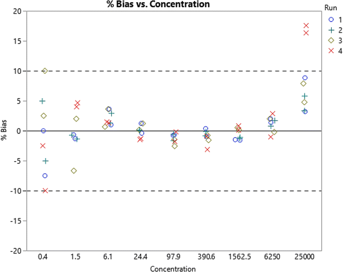
Robustness is an important aspect of a bioanalytical method and is influenced by both the standard curve range as well as the quantitation range. The quantitation range is from the LLOQ to the ULOQ of a method; the standard curve range may include additional points which improve the fit. When below the LLOQ or above the ULOQ, they are commonly referred to as anchor points. For simplicity in the following case study, all such points will be referred to as auxiliary points. The application of %bias plots is a practical approach to establishing the quantitation range and to judge the usefulness of auxiliary points. These are also functional tools in the selection and assessment of curve fitting and weighting models. Below is an example which provides a step-by-step approach to the establishment of the standard curve and the quantitation ranges as well as to the selection of a regression model. The assumption in the examples presented below is that assay conditions are optimized. The definition of the %bias used in the example below is as follows:

$$ \%\mathrm{Bias}=\frac{\mathrm{Determined}\ \mathrm{Concentration}\hbox{--} \mathrm{Nominal}\ \mathrm{Concentration}}{\mathrm{Nominal}\ \mathrm{Concentration}}\times 100 $$

• 1. For the initial assessment of the range, visually examine the concentration response relationship from an original development run on a semi-log scale. Note that a log-log scale artificially minimizes the curvature of the response and makes it difficult to estimate the expected sensitivity.

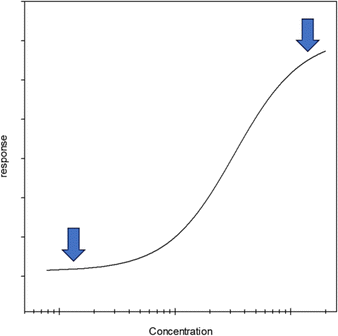
• 2. Determine the positions of the upper and lower asymptotes pointed out by arrows in the figure below.

  

• 3. Determine the concentration of 10 individual points that span the distance between the lower and upper asymptotes. These should be approximately equally spaced on the log scale. Once prepared, these will be considered mock standards.

  

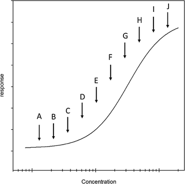
• 4. Prepare four independent sets of mock standards; it is useful to have two analysts prepare two sets each. Each set of mock standards should be added to an assay plate in duplicate wells.

  

The plot above indicates that the quantification range (LLOQ to ULOQ) should be 1.5 and 6250.

• 5. At this point, remove the standards with the highest bias, re-fit, and re-plot the data.

  

• 6. According to guidance, bias of up to 25% is allowed at the LLOQ level; however, a tighter bias acceptance would be beneficial when fitting a model to the standards. In the example provided here, standards with bias less than 5% appear to make for a suitable quantification range; therefore, the proposed LLOQ would be 1.5 and the ULOQ, 6250.

  

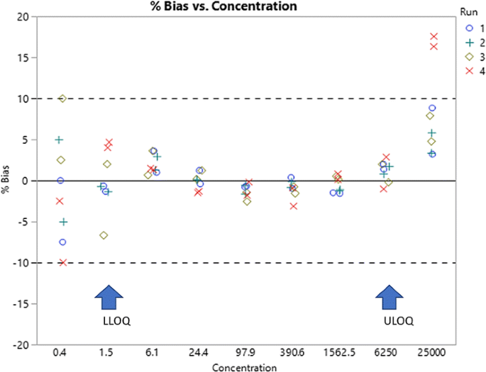
At this stage of the analysis, there are anchor points at 0.4 and 25,000. After further analysis, these may be removed, and the data re-regressed to assess whether the fit of the standards within the quantitation range has improved. This is judged by reduction in the %bias across the quantitation range.

Assessing Curve Fitting Models

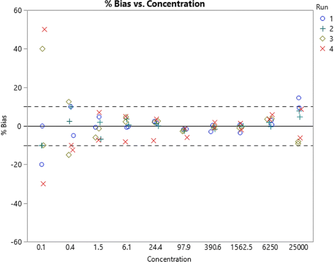
An example is provided in Fig. 4a below to demonstrate an approach to establishing the best curve fitting model. In this example, two analysts each prepared two standard curves. The standard curves were independently run on four different plates. The curves were fitted to either a 4 PL or 5 PL model, and %bias was determined. Figure 4b is plot of concentration against the response (OD) for each of the four standard curves in Fig. 4b and demonstrates that there is no appreciable difference between the 4 and 5 PL fits. The data also suggest that the 5 PL fit may have provided for more homogeneity around zero. The 4 PL fit has a somewhat of a curvature. A review of the standard curve data shows that in this range, the assay does not display an upper asymptote suggesting that 5 PL regression may provide a better fit.

Fig. 4

a 5 PL fit. Four standard curves prepared independently by two analysts. The curves were subsequently fitted to 4 PL and 5 PL regression. %Bias were determined and plotted against the concentration. b 4 PL fit. A plot of concentration versus absorbance (OD) for the four standard curves presented in part a

In the above example, the 5 PL fit was shown to be preferable over the 4 PL fit by showing homogeneity of the %bias around zero across the qualification range.

Appendix 2. Validation of Software for Non-Linear Regression

Validation is laboratory specific, and one should follow the validation and risk management standard procedures of the laboratory over the course of the instrument system life cycle. An overall validation guideline covering the general validation principles can be found in the US FDA guidance below:

US FDA, General Principles of Software Validation: Final Guidance for Industry and FDA Staff, January 2002 (30).

This guidance has defined software validation as confirmation by examination and provision of objective evidence that software specifications conform to user needs and intended application and that the particular requirements implemented through software can be consistently fulfilled.

There are several recommended, up-to-date international and US-based guidelines and regulations for software validation and qualification. The most recent guidance documents (some in draft stage) address current industry trends, practices, and expectations to assure successful compliance with internal and external regulators. Here is a list:

• OECD SERIES on Principles of Good Laboratory Practice and Compliance Monitoring, Application of GLP Principles to Computerised Systems, Number 17, Apr 2016. (31)

• U.S. FDA, Title 21 of the U.S. Code of Federal Regulations: 21 CFR 11 “Electronic Records; Electronic Signatures”, Aug 2003. (32)

• U.S. Pharmacopeial Convention 42(3) In-Process Revision: 〈1058〉 ANALYTICAL INSTRUMENT QUALIFICATION. Publish date: April 2016 (33)

• MHRA GMP Data Integrity Definitions and Guidance for Industry, Draft Version for consultation, July 2016 (34)

• DRAFT PIC/S, Good Practices for Data Management and Integrity in Regulated GMP/GDP Environments, Aug 2016 (35)

The following are a series of steps and suggestions to consider; these are known as the 4Q model: Design Qualification (DQ), Installation Qualification (IQ), Operational Qualification (OQ), and Performance Qualification (PQ).

Assess the vendor prior to purchase for compliance requirements and capabilities to install and support the instrument and software. Work with the vendor to establish the specifications to be used in the instrument qualification process. Include a review of the vendor software testing and other requirements (for example, those in Performance and Validation Requirements for Non-Linear Regression Software section with the assessment. Establish the scope of intended use. The vendor is responsible for enabling your subsequent instrument qualification and software validation phases. This is your DQ.

The next steps approximate the IQ and OQ phases. Following purchase, configure the instrument and perform an IQ and OQ of the instrument. Install and configure the software and interfaces and perform a software installation qualification. Lock down the hardware and software components such as the computer, network, and interfaces of the system to establish a base state and perform change control beyond this point. Establish the reproducibility of sample analysis (e.g., method development) and assess the software and compliance requirements (including curve fitting). Finally, establish and document the entire data flow process with data integrity controls for example in a draft SOP.

The last steps are comparable to a PQ phase. The software validation testing or intended use as directed by the validation plan can begin and will include the documented verification of the capabilities (or requirements) from Performance and Validation Requirements for Non-Linear Regression Software section. A report verifying each step in your plan is necessary and could combine the instrument qualification and system validation summaries or leave them in separate reports. SOPs should at this point be finalized and the system released for production use. At this stage, a method validation can be completed, and this would initiate the instrument PQ phase or ongoing checks and tests for routine study sample analysis. In parallel, the software maintenance phase (i.e., periodic reviews, change control, access control, data archiving) will commence.

Appendix 3. Anchor Points

Table II provides example of a calibration curve with the targeted quantitative range of 1.53 to 400 ng/mL, with and without the benefit of lower anchor points. Here, unweighted 5 PL regression model has been used, and individual accuracy values in %RE have been listed for each calibrator point. RE values are presented with one, two, and three lower anchor points as well as with no anchor points. As shown in this table, the accuracy of the targeted LLOQ of the assay (1.53 ng/mL;) is improved with inclusion of lower anchor points. In this example, anchor points help the LLOQ of the assay pass. In fact, 1.53 ng/mL calibrator would only pass the RE acceptance criterion when a minimum of two anchor points are included in the curve. Similarly, anchor points above and beyond the ULOQ of the assay may also be evaluated for their impact. It should be noted that placement of upper anchor points in the prozone would disrupt the regression and should be avoided.

Table II Example Calibration Curve With and Without the Benefit of Lower Anchor Points

Appendix 4. Editing a Calibration Curve

Table III provides example of a calibration curve with quantitative range of 0.156 to 20 ng/mL where multiple calibrators have failing CV or REs. In this example, after masking the 5 ng/mL calibrator whose CV fails, the REs of a number of other calibrators, including the targeted LLOQ of assay, are brought into the acceptance range and pass. As a result, no additional masking was required. The calibrator CV and RE values before and after masking of the 5 ng/mL calibrator are shown in this table, and the trend in %RE values are graphically presented in Fig. 5. In contrast and as an example, masking of the 0.625 ng/mL calibrator which had the second highest CV did not appreciably improve the curve (data not shown).

Table III Impact Masking of a Failed Calibrator on the Curve Fit. The CVs and REs of individual calibrators before and after masking a failed calibrator (5 ng/mL) are listed in this table. Masking of the 5 ng/mL calibrator which failed CV criteria brings REs of 0.625, 0.313, and 0.156 ng/mL calibrators within the acceptance range of ± 20%. NQ non-quantifiable. ^ªCV exceeds acceptance limit of < 20%

Fig. 5

Masking a failed calibrator and impact on the curve fit. A graphic representation of the impact of masking the 5 ng/mL calibrator which had failed CV and RE criteria on the RE and CVs of other calibrators. This graph demonstrates that masking one calibrator (5 ng/mL) brings the REs of the majority of calibrators within the acceptance range. An example for the assessment of curve fitting models is provided in Appendix 1

Appendix 5. Zero Calibrator and Blank Sample

Blank and zero samples have distinct definitions in chromatographic assays, but in LBAs, the two are synonymous terms. The LBA zero calibrator or the blank is unfortified matrix.

Zero Calibrators as Anchor Points

As stated previously, the zero calibrator is not required, but if included, it should be treated as an anchor point. The decision for inclusion or exclusion of zero in the curve fit should be based on its impact on the performance of the assay during method development. Kelley et al. (7) have presented a case for inclusion of zero in the regression. At the same time, the 2012 EMA bioanalytical guidance (9) provided the recommendation that the zero calibrator not be included in the calculation of calibration curve parameters in chromatographic assays. It is not clear whether this latter directive also encompasses the LBAs. An example curve regressed with and without the zero calibrator is presented in Table IV where the measured concentrations of validation samples and their respective RE values have been plotted. Here, inclusion or omission of the zero calibrator does not make appreciable difference in the accuracy of the ULOQ, HQC, MQC, or LQC samples, but it impacts the performance of the 3.125 ng/mL LLOQ samples. Without the zero calibrator, two out of three LLOQ samples fail the targeted RE acceptance criterion of ± 25% which disqualifies 3.125 ng/mL for LLOQ. On the other hand, if zero calibrator is included in the regression, all three LLOQ validation samples meet the targeted RE criterion in this example. In other cases, inclusion of zero has proven to improve the performance of more than one level of validation samples although this impact has not been consistent across methods. As such, it is suggested that the impact of the zero calibrator on the curve fit as well as on the extrapolated concentrations of the quality controls be assessed during method development and subsequently confirmed in the validation phase and documented in the test method.

Table IV Comparison of Validation Sample Performance Against Curves Regressed With and Without Zero Calibrator

There has been much discussion about the guiding rules for subtraction of the blank. It is the collective recommendation of the authors that calibrators are not corrected for either the blank response or the blank measured concentration.

References

Findlay JWA, Dillard RF. Appropriate calibration curve fitting in ligand binding assays. AAPS J. 2007;9(2):E260–7. https://doi.org/10.1208/aapsj0902029.
Findlay JWA, Smith WC, Lee JW, Nordblom GD, Das I, DeSilva BS, et al. Validation of immuoassays for bioanalysis: a pharmaceutical industry perspective. J Pharm Biomed Anal. 2000;21(6):1249–73. https://doi.org/10.1016/S0731-7085(99)00244-7.
Jani D, Allinson J, Berisha F, Cowan KJ, Devanarayan V, Gleason C, et al. Recommendations for use and fit-for-purpose validation of biomarker multiplex ligand binding assays in drug development. AAPS J. 2016;18(1):1–14. https://doi.org/10.1208/s12248-015-9820-y.
DeSilva B, Smith W, Weiner R, Kelley M, Smolec J, Lee B, et al. Recommendations for the bioanalytical method validation of ligand-binding assays to support pharmacokinetic assessments of macromolecules. AAPS J. 2003;20(11):1885–900.
Kelley M, DeSilva B. Key elements of bioanalytical method validation for macromolecules. AAPS J. 2007;9(2):E156–63. https://doi.org/10.1208/aapsj0902017.
Booth B, Arnold ME, DeSilva B, Amaravadi L, Dudal S, Fluhler E, et al. Workshop report: crystal city V-quantitative bioanalytical method validation and implementation: the 2013 revised FDA guidance. AAPS J. 2015;17(2):277–88. https://doi.org/10.1208/s12248-014-9696-2.
Kelley M, Stevenson L, Golob M, Devanarayan V, Pedras-Vanconcelos J, Staak RF, et al. Workshop report: AAPS workshop on method development, validation, and troubleshooting of ligand binding assays in the regulated environment. AAPS J. 2015;17(4):1019–24. https://doi.org/10.1208/s12248-015-9767-z.
O’Hara DM, Theobald V, Egan AC, Usansky J, Krishna M, TerWee J, et al. Ligand binding assays in the 21st century laboratory: recommendations for characterization and supply of critical reagents. AAPS J. 2012;14(2):316–28. https://doi.org/10.1208/s12248-012-9334-9.
EMA, European Medicines Agency. Guideline on bioanalytical method validation. [Online] July 21, 2011. EMEA/CHMP/EWP/192217/2009.
U.S. Food and Drug Administration. Guidance for industry bioanalytical method validation. [Online] May 2001. http://www.fda.gov/cder/guidance/index.htm.
U.S. Food and Drug Administration, US Department of Health and Human Services. Draftguidance for industry: bioanalytical method validation (Revised).[Online] September 2013. http://www.fda.gov/downloads/Drugs/GuidanceComplianceRegulatoryInformation/Guidances/UCM368107.pdf.
Guideline on bioanalytical method validation in pharmaceutical development. Japan: Pharmaceutical Manufacturers Association; 2013.
Guide for validation of analytical and bioanalytical methods, Resolution - RE n. 899, of May 29, 2003, Agência Nacional de Vigilância Sanitária. www.anvisa.gov.br.
Bioanalytical Guidance Resolution – RDC # 27 of 17 MAY 2012, Agência Nacional de Vigilância Sanitária. www.anvisa.gov.br.
Viswanathan CT, Bansal S, Booth B, DeStafano J, Rose MJ, Sailstad J, et al. Quantitative bioanalytical methods validation and implementation: best practices for chromatographic and ligand binding assays. PharmRes. 2007;24(10):1962–73.
Nowatzke W, Woolf E. Best practices during bioanalytical method validation for the characterization of assay reagents and the evaluation of analyte stability in assay standards, quality controls, and study samples. AAPS J. 2007;9(2):F117–E122.
Smolec JM, DeSilva B, Smith W, Weiner R, Kelly M, Lee B, et al. Workshop report—bioanalytical method validation for macromolecules in support of pharmacokinetic studies. Pharm Res. 2005;22(9):1425–31. https://doi.org/10.1007/s11095-005-5917-9.
Yang H, Kim HJ, Zhang L, Strouse RJ, Schenerman M, Jiang XR. Implementation of parallelism testing for four-parameter logistic model in bioassays. Pharm Sci Technol. 2012;66(3):262–9. https://doi.org/10.5731/pdajpst.2012.00867.
Sondag P, Joie R, Yang H. Comment and completion: implementation of parallelism testing for four-parameter logistic model in bioassays. PDA J Pharm Sci Tech. 2015;69(4):467–70.
Sondag P. Comparison of methodologies to assess the parallelism between two four parameters logistic curves. In: NonClinical Statistics Conférence. October 2014. Bruges, Belgium. http://www.ncsconference.org/?page_id=409.
Boulanger B, Devanarayan V, Dewé W. Statistical considerations in the validation of ligand-binding assays. In: Khan MN, Findlay JWA editors. Ligand binding assay: Development, Validation, and Implementation in the Drug Development Arena. Wiley; 2010. p. 111–128.
Hubert P, Nguyen-Huu J-J, Boulanger B, Chapuzet E, Chiap P, Cohen N, et al. Harmonization of strategies for the validation of quantitative analytical procedures: a SFSTP proposal—part I. J Pharma Biomed Anal. 2004;36(3):579–86.
Bortolotto E, Rousseau R, Teodorescu B, Wielant A, Debauve G. Assessing similarity with parallel-line and parallel-curve models: implementing the USP development/validation approach to a relative potency assay. Bioprocess International. 2015;13(6):26–37.
O’Connell MA, Belanger BA, Haaland PD. Calibration and assay development using the four-parameter-logistic model. Chemom Intell Lab Syst. 1993;20(2):97–114. https://doi.org/10.1016/0169-7439(93)80008-6.
Gottschalk PG, Dunn JR. The five-parameter logistic: a characterization and comparison with the four-parameter logistic. Anal Biochem. 2005;343(1):54–65. https://doi.org/10.1016/j.ab.2005.04.035.
Sadler WA, Smith MH. Estimation of the response-error relationship in immunoassay. Clin Chem. 2005;31(11):1802–5.
Hawkins DM. The problem of overfitting. J Chem Info Compu Sci. 2004;44(1):1–12. https://doi.org/10.1021/ci0342472.
Mantanus J, Ziémons E, Lebrun P, Rozet E, Klinkenberg R, Streel B, et al. Active content determination of non-coated pharmaceutical pellets by near infrared spectroscopy: method development, validation and reliability evaluation. Talanta. 2010;80(5):1750–7. https://doi.org/10.1016/j.talanta.2009.10.019.
Anscombe FJ. Graphs in statistical analysis. Am Stat. 1973;27(1):17–21.
US Food and Drug Administration. General principles of software validation: final guidance for industry and FDA staff. 2002.