
Abstract
A next step in development of the KrkNLO method of including complete NLO QCD corrections to hard processes in a LO parton-shower Monte Carlo is presented. It consists of a generalisation of the method, previously used for the Drell–Yan process, to Higgs-boson production. This extension is accompanied with the complete description of parton distribution functions in a dedicated, Monte Carlo factorisation scheme, applicable to any process of production of one or more colour-neutral particles in hadron–hadron collisions.
1 Introduction
The method of including complete NLO QCD corrections to hard processes in the LO parton-shower Monte Carlo (PSMC), nicknamed KrkNLO, was originally proposed in Ref. [1], where its first numerical implementation on top of a toy-model PSMC was also presented. It was restricted there to gluon emission only and was elaborated for two processes: \(Z/\gamma ^*\) production in hadron–hadron collisions, i.e. the Drell–Yan (DY) process and deep inelastic electron–hadron scattering (DIS).
In Ref. [2], the KrkNLO method was implemented for \(Z/\gamma ^*\) production process at large hadron collider (LHC) in combination with Sherpa [3] and Herwig++ [4,5,6] PSMCs. Many NLO-class numerical results (distributions of transverse momenta, rapidity, integrated cross sections, etc.) were presented there and comparisons of the KrkNLO predictions with those from other methods, such as MC@NLO [7] and POWHEG [8], were also performed.
The main advantage of the KrkNLO method with respect to other, older methods of matching the fixed-order NLO calculations with PSMCs (MC@NLO and POWHEG) is its simplicity. This simplicity stems from the fact that the entire NLO corrections are implemented using a simple positive multiplicative MC weight. However, in order to profit from it, one has to use in the KrkNLO method parton distribution functions (PDFs) in a special, so-called Monte Carlo (MC) factorisation scheme and PSMC has to fulfil some minimum quality criteria. Most of modern PSMCs [9,10,11,12,13] are good enough for the KrkNLO method.
Construction of PDFs in the MC factorisation scheme (FS) has evolved step by step: in Ref. [1] it was defined for gluonstrahlung only (albeit for two different processes, DY and DIS). In Ref. [2], the KrkNLO PDFs in the MC FS were defined and numerically constructed including also gluon to quark transitions/splittings, relevant for the complete NLO corrections in the DY process, which at the LO level has only quarks and antiquarks in the initial state. PDFs in the MC scheme in Ref. [2] were defined in terms of the standard \(\overline{\text {MS}}\) PDFs, and constructed numerically by transforming the \(\overline{\text {MS}}\) PDFs into MC-scheme PDFs, before they were plugged into PSMC used in the KrkNLO method.
However, in Ref. [2] certain elements in the transition matrix K, transforming the \(\overline{\text {MS}}\) PDFs into the MC-scheme PDFs could be omitted, because they were not relevant (i.e. of a NNLO class) for the DY process. These elements of the transition matrix have to be added for any process with initial-state gluons, such as the Higgs-boson production elaborated in the present work. They will be defined and applied in the following, such that the complete transition matrix K transforming the \(\overline{\text {MS}}\) PDFs into the MC-scheme PDFs will be specified for the first time. It will be argued that PDFs in such a MC-scheme can serve in the KrkNLO method for any process at a hadron–hadron collider in which a colour-neutral single or multiple system of heavy particles is produced. For other processes, with one or more coloured partons in the final state at LO level, the KrkNLO method with PDFs in the MC scheme may also work, but this subject is reserved for the forthcoming publications.
The MC factorisation scheme is a complete scheme, such that NLO coefficient functions for any hard process under consideration are known, hence PDFs in the MC FS can be fitted directly to experimental DIS and DY data. However, at present, we obtain them from PDFs in the \(\overline{\text {MS}}\) scheme and leave out direct fitting to data for the future developments.
On the methodological side, as seen in Refs. [1, 2], the essence of the KrkNLO method is that certain NLO correction terms in an unintegrated/exclusive form present in the \(\overline{\text {MS}}\) scheme, which are proportional to unphysical Dirac-delta terms in transverse momentum of emitted real partons, are removed in the KrkNLO methodology by means of redefinition of PDFs from the \(\overline{\text {MS}}\) to MC scheme. These ‘pathological’ terms are preventing the use of a simple multiplicative MC weight for implementing NLO corrections in the \(\overline{\text {MS}}\) scheme in real-emission phase space, and they complicate implementation of the MC@NLO and POWHEG methods. These peculiar terms can be determined and calculated either by means of studying the NLO corrections to hard process (coefficient functions), or, alternatively, by means of integrating soft-collinear counter-terms (similar to these in the Catani–Seymour method [14]), which define the MC-scheme PDFs in \(d=4+2{\varepsilon }\) dimensions.Footnote 1 We are going to calculate them using both methods, obtaining the same results.
Last but not least, the NLO calculations for the DY process of Ref. [2] were also compared with the NNLO calculations of MCFM [15], leading to the conclusion that they are closer to the latter than the results of the MC@NLO and POWHEG methods.
The outline of the paper is the following: in Sect. 2 the KrkNLO method is characterised briefly. In Sect. 3 all distributions needed for implementation of the KrkNLO method for Higgs-boson production in gluon–gluon fusion are elaborated, including also many analytical crosschecks and a necessary update of the virtual corrections in soft-collinear counter-terms used in Ref. [2] for the \(Z/\gamma ^*\) (DY) process. Section 4 presents numerical results for PDFs in the MC scheme. Then the first numerical results for the total cross section from the KrkNLO method for the Higgs production at the LHC are shown in Sect. 5. Finally, in Sect. 6 we summarise the paper and discuss future prospects of our work. In Appendix A the formulae for the NLO coefficient functions of the DIS process in the MC scheme are provided.
2 The method
The KrkNLO method was formulated in a few variants. For instance, in the version of Ref. [1], the MC weight implementing the NLO corrections sums the contributions from all relevant partons generated in PSMC next to the hard process “democratically”, such that it works equally well for PSMCs based on angular ordering or virtuality ordering, contrary to POWHEG which requires adding extra gluons to a PSMC event. In the present work, we are going to follow the variant of KrkNLO discussed in Ref. [2], in which the NLO-correcting MC weight uses only one parton, the one closest to the hard process in the transverse momentum, that is, the first parton generated in the backward evolution (BEV) in the PSMC algorithm with \(k_T\)-ordering.
In any case, in the KrkNLO method, the entire event of PSMC is preserved and reweighted, contrary to POWHEG and MC@NLO where the parton attributed to the hard process is generated outside PSMC and, only later on, the remaining partons are provided by PSMC. Obviously, this puts certain minimum quality requirements on the PSMC: (i) the first parton in the BEV algorithm has to be generated with the distribution which has a correct soft and collinear limit and (ii) its phase space in momentum and flavour space has to be covered completely, without empty regions. Luckily, the above requirement is fulfilled by all modern PSMCs for initial-state emissions discussed in this work.
It is worth to comment in advance on the apparent use in the following of the soft-collinear counter-terms (dipoles) of the Catani–Seymour (CS) subtraction scheme [14]. Their role is twofold: (1) the CS dipoles serve us as a useful benchmark, as they provide a reference model for QCD distributions of real emissions featuring the exact soft and collinear limits and (2) the CS scheme helps us in a proper inclusion of the NLO virtual corrections. However, let us point out immediately an important difference between the MC and CS scheme: the CS dipoles do not include virtual corrections, while soft-collinear counter-terms (SCCTs) of the KrkNLO do include them, albeit not calculated from Feynman diagrams, but deduced from PDF momentum sum rules. The role of the SCCTs in the KrkNLO methodology is also much richer than that of the dipoles in the CS scheme—our SCCTs not only provide subtractions of soft-collinear singularities in real-emission phase space, but they are also used to define PDFs in the MC factorisation scheme. Moreover, their sums are required to coincide with the corresponding sums of real-parton distributions in PSMC.Footnote 2
3 Higgs production in gluon–gluon fusion
In the following we are going to collect all distributions needed for implementation of the KrkNLO method for the gluon-fusion Higgs production in hadron–hadron collisions. Elements of the matrix transforming PDFs from the \(\overline{\text {MS}}\) to MC scheme will also be obtained as a byproduct.
We start necessarily from the leading order (LO) process
see Fig. 1, where \(Q = p_1 + p_2\). The LO matrix element squared, in the limit \(m_t \rightarrow \infty \) and neglecting all other quarks contributions, reads
where \(v^2 = (\sqrt{2}G_F)^{-1}\) is the Higgs vacuum expectation value (VEV) squared. Hence, the LO total cross section takes the form
For all NLO subprocesses (channels)
where a and b are incoming partons (gluons and/or quarks), while c is an outgoing parton (quark or gluon) we shall use the same parametrisation of the kinematics in terms of the following Sudakov variables:

The LO Feynman diagram for the process of Higgs boson production in gluon–gluon fusion. The effective vertex (black dot) corresponds to a quark loop with summation over all quarks, in which the top-quark mass is set to infinity while the masses of the other quarks are set to zero
For the gg-channel NLO subprocess
shown in Fig. 2, the matrix element squared reads
For the qg-channel NLO subprocess
shown in Fig. 3, one obtains
Finally, for the \(q\bar{q}\) channel
see Fig. 4, one has
This last process, unlike the previous ones, is not generated by the backward-evolution PSMC starting from the \(gg\rightarrow H\) hard process, hence in the KrkNLO method, its contribution cannot be treated by NLO-reweighting of events generated by the main branch of the LO PSMC algorithm. It has to be added as an extra tree-level LO process to PSMC. Moreover, it is free of collinear and soft singularities. This poses no problem as most of present-day PSMCs implement such a process.

The NLO Feynman diagrams for real-parton radiation in the process of Higgs-boson production in gluon–gluon fusion: the gg channel
3.1 CS dipoles and MC matrix elements
In the following we shall elaborate mainly on the hadron–hadron collision producing the Higgs boson or \(Z/\gamma ^*\) (Drell–Yan process). However, components of the KrkNLO method defined here will also be applicable to any LO process \(a+\bar{a} \rightarrow X\) and the corresponding \( a+b \rightarrow X+c\) where \(X=H, Z/\gamma , W^\pm , ZZ, W^+W^-\) or any other colour-neutral heavy object; \(a,b=q,\bar{q},g\) are initial coloured partons and c is an additional parton emitted at the NLO level.

The NLO Feynman diagram for real-parton radiation in the process of Higgs-boson production in gluon–gluon fusion: the gq channel

The NLO Feynman diagram for real-parton radiation in the process of Higgs-boson production in gluon–gluon fusion: the \(q\bar{q}\) channel
In the following formulation of the KrkNLO-method components, the CS dipoles will serve us as useful auxiliary objects. They are formed by an initial-state (on-shell) emitter a from one hadron and a spectator parton b from another hadron,Footnote 3 see Fig. 5. Following closely the notation of the CS work [14], the emitter a splits into an off-shell \(\widetilde{ac}=\bar{b}\) entering into the hard process and an emitted parton c. The CS dipoles \(\mathfrak {D}^{(ac,b)}\) relevant for processes of our interest are proportional to \(\bar{P}_{ \widetilde{ac} ,a}\), the DGLAP kernel for the \( a\rightarrow \widetilde{ac}\) splitting.Footnote 4
For the processes of the annihilation \(a\bar{a} \rightarrow X\) at the LO level, such as the Higgs production and the DY process, in each NLO channel \(ab \rightarrow cX \) we must have \( \widetilde{ac} =\bar{b}\) in the NLO splitting. In other words, the NLO splitting in the annihilation processes is fully determined by a and b.Footnote 5 The above rules are illustrated in Fig. 5 and possible indices are listed in Table 1 for the emission from the incoming line a.Footnote 6
Let us first define explicitly the MC distributions (matrix elements) and the CS dipoles representing the initial-state real-parton emissions for the Higgs production process in \({d}=4+2{\varepsilon }\) dimensions:
-
(A)
For the \(g + g \rightarrow H + g\) channel a typical/representative distribution of PSMC, summing the emissions from both incoming gluons, is
$$\begin{aligned} |\mathcal{M}_{gg\rightarrow Hg}^{\text {MC}}|^2 = 8\pi \alpha _s\,\mu ^{-2\epsilon }\,\frac{1}{Q^2}\, \frac{1}{\alpha \beta }\,(1-z)\hat{P}_{gg}(z;\epsilon ) |\mathcal{M}_{gg\rightarrow H}^{\text {LO}}|^2,\nonumber \\ \end{aligned}$$(3.12)where the \(g\rightarrow g\) splitting function is given by
$$\begin{aligned} \hat{P}_{gg}(z;\epsilon )= & {} 2C_A\left[ \frac{z}{1-z} + \frac{1-z}{z} + z(1-z)\right] \nonumber \\= & {} C_A\frac{1 + z^4 + (1-z)^4}{z(1-z)}. \end{aligned}$$(3.13)It is equal to the sum of two CS dipoles \( |\mathcal{M}_{gg\rightarrow Hg}^{\text {MC}}|^2 = \mathfrak {D}^{(gg,g)} _{(1)}+ \mathfrak {D}^{(gg,g)}_{(2)}\), where
$$\begin{aligned}&\mathfrak {D}^{(gg,g)}_{(1)}= \frac{\alpha }{\alpha +\beta } |\mathcal{M}_{gg\rightarrow Hg}^{\text {MC}}|^2, \quad \mathfrak {D}^{(gg,g)}_{(2)}= \frac{\beta }{\alpha +\beta } |\mathcal{M}_{gg\rightarrow Hg}^{\text {MC}}|^2,\nonumber \\ \end{aligned}$$(3.14)with soft partition functions \( \frac{\alpha }{\alpha +\beta }\) and \(\frac{\beta }{\alpha +\beta }\) separating the soft singularity evenly between two incoming emitters. Indices (1) and (2) are used to distinguish the above two dipoles.
-
(B)
For the \(g + q \rightarrow H + q\) channel we have (with a single soft-collinear pole the soft partition functions are not needed):
$$\begin{aligned}&|\mathcal{M}_{gq\rightarrow Hq}^{\text {MC}}|^2 = \mathfrak {D}^{(qq,g)}_{(1)} =8\pi \alpha _s\,\mu ^{-2\epsilon }\,\frac{1}{Q^2}\, \frac{1}{\alpha }\,\hat{P}_{gq}(z;\epsilon ) |\mathcal{M}_{gg\rightarrow H}^{\text {LO}}|^2,\nonumber \\ \end{aligned}$$(3.15)where the \(q\rightarrow g\) splitting function reads
$$\begin{aligned}&\hat{P}_{gq}(z;\epsilon ) = C_F\left[ \frac{1 + (1-z)^2}{z} + \epsilon \, z\right] . \end{aligned}$$(3.16) -
(C)
Finally, for the \(g + \bar{q} \rightarrow H + \bar{q}\) channel, the CS dipole and MC distribution is the same as the previous one for quarks.
The above distributions agree with these used in the POWHEG-method construction of Ref. [16].
For the sake of completeness, let us collect the CS dipoles and MC distributions already known from Refs. [1, 2], with the \(q\rightarrow q\) and \(g\rightarrow q\) splittings. They will be needed in the following to define the transition matrix K from the \(\overline{\text {MS}}\) to MC factorisation scheme for all PDFs.
-
(A)
For the \(q + \bar{q} \rightarrow Z + g\) channel, the MC distribution reads
$$\begin{aligned} |\mathcal{M}_{q\bar{q}\rightarrow Zg}^{\text {MC}}|^2&= \mathfrak {D}^{(q g ,\bar{q})}_{(1)} +\mathfrak {D}^{(\bar{q} g ,q)}_{(2)} = 8\pi \alpha _s\,\mu ^{-2\epsilon }\,\frac{1}{Q^2}\,\nonumber \\&\quad \times \frac{1}{\alpha \beta }\,(1-z)\hat{P}_{qq}(z;\epsilon ) |\mathcal{M}_{q\bar{q}\rightarrow Z}^{\text {LO}}|^2, \end{aligned}$$(3.17)where
$$\begin{aligned} \hat{P}_{qq}(z;\epsilon ) = C_F\left[ \frac{1+z^2}{1-z} + \epsilon (1-z) \right] , \end{aligned}$$(3.18)and the soft partition function is used again:
$$\begin{aligned}&\mathfrak {D}^{(qg ,\bar{q})}_{(1)} = \frac{\alpha }{\alpha +\beta } |\mathcal{M}_{q\bar{q}\rightarrow Zg}^{\text {MC}}|^2, \quad \mathfrak {D}^{(\bar{q}g ,q)}_{(2)} = \frac{\beta }{\alpha +\beta } |\mathcal{M}_{q\bar{q}\rightarrow Zg}^{\text {MC}}|^2.\nonumber \\ \end{aligned}$$(3.19) -
(B)
For the \(q + g \rightarrow Z + q\) channel we have (the soft partition function in the MC distribution is not necessary):
$$\begin{aligned}&|\mathcal{M}_{qg\rightarrow Zq}^{\text {MC}}|^2 = \mathfrak {D}^{(gq ,q)}_{(1)} = 8\pi \alpha _s\,\mu ^{-2\epsilon }\,\frac{1}{Q^2}\, \frac{1}{\alpha }\,\hat{P}_{qg}(z;\epsilon ) |\mathcal{M}_{q\bar{q}\rightarrow Z}^{\text {LO}}|^2,\nonumber \\ \end{aligned}$$(3.20)where
$$\begin{aligned} \hat{P}_{qg}(z;\epsilon ) = T_R\left[ z^2 + (1-z)^2 + 2\epsilon \, z(1-z)\right] . \end{aligned}$$(3.21)
It should be stressed that all the above MC distributions and CS dipoles are basically in the exclusive (unintegrated) form.
All the above relations between the MC distributions and the exclusive MC/CS counter-terms for any annihilation processes can be summarised in a compact formula as follows:
where translation from the indices (ab) to (abc) is unique for a given annihilation process and for a given initial parton splitting, as demonstrated explicitly in Table 1 for the splitting of the initial parton a, see also Fig. 5. Moreover, on the RHS of the above relation only one of \(\mathfrak {D}\)’s is nonzero, except for the \(c=g\) case (gluonstrahlung), but in this case both \(\mathfrak {D}\)’s are equal. Hence, there is in practice one-to-one correspondence \((ab) \leftrightarrow (abc)\) for all annihilation processes, to be often exploited in the following section.
3.2 Integrated CS dipoles and counter-terms of MC scheme
For the purpose of installing virtual parts (using PDF momentum sum rules) in the MC distributions (soft-collinear counter-terms) and defining the K-matrix for transforming PDFs from the \(\overline{\text {MS}}\) to MC scheme, we need to integrate partly all distributions defined in the previous subsection, keeping the \(z=1-\alpha -\beta \) variable fixed.
A z-dependent differential cross section corresponding to the real-emission MC matrix elements can be expressed in the following way:
where \(\hat{\Gamma }^{\text {MC}}_{ab,R}(z,\epsilon )\) is the MC real-emission function corresponding to the partly integrated MC distribution of the previous subsection for a given process: \(a+b \rightarrow X+c\). The integration element \(\mathrm{d}\hat{\Phi }\) can be expressed in terms of the Sudakov variables as follows:
The above expressions are defined in \(\mathrm{d} = 4 + 2\epsilon \) dimensions in order to regularise, in the usual way, the soft and collinear singularities of the real-parton radiation.
Using the exact NLO matrix element, one can similarly write, for each channel ab, a regularised partly integrated NLO cross section for real-parton emission:
Following Eq. (3.22), one may also define the relation of the integrated MC distribution to the individual integrated soft-collinear counter-terms:
where \(\hat{\Lambda }_R\) are the corresponding integrals \(\int \mathrm{d}\hat{\Phi }\; \mathfrak {D}\) as in Eq. (3.23). However, contrary to the CS counter-terms, the counter-terms \(\hat{\Lambda }^{\text {MC}}\) of the MC scheme (and the \(\hat{\Gamma }^{\text {MC}}\) radiation functions as well) will also include virtual corrections, calculated using the momentum sum rules, see next subsections for details.
Let us calculate all the above objects in more detail for the \(gg\rightarrow Hg\) channel and then, skipping details of analytical integration, for other channels.
3.3 \(gg \rightarrow Hg\) channel
A real-emission part of the MC radiation function results from the following integration:Footnote 7
Using the standard expansion \( (1-z)^{-1+2\epsilon } = \frac{1}{2\epsilon }\delta (1-z) + \big (\frac{1}{1-z}\big )_+ + 2\epsilon \big (\frac{\ln (1-z)}{1-z}\big )_+ \) we obtain
The NLO real correction according to Ref. [17] reads
From the above equations we readily obtain the NLO real coefficient function in the MC scheme:
The same expression is obtained in 4 dimensions by means of performing first the MC-dipole subtraction and then integrating the finite result over the phase space:
A virtual correction to the above MC radiation function \(\hat{\Gamma }_{gg}\) is calculated from the momentum sum rules:
where \(n_f\) is the number of fermions. The first part in the above virtual correction resulting from integration over the first term in brackets on RHS reads as follows:
In order to calculate the second part to the virtual correction in RHS of Eq. (3.32) we need to know first the following MC radiation functions for the \(g \rightarrow q\) transition, e.g. from the process \(q + g \rightarrow Z + q\):
where \(|\mathcal{M}_{qg\rightarrow Zq}^{\text {MC}}|^2\) is shown in Eq. (3.20).
Using the above result we can cross-check the formula for the gluon-channel MC radiation function of the DY process calculated previously in 4 dimensions in Ref. [2]. For the exact NLO contribution Ref. [18] provides
Then the resulting coefficient function for the DY process in the MC scheme reads
which agrees with our previous result, given in Ref. [2].
For the sake of completeness, the corresponding coefficient function in the \(\overline{\mathrm{MS}}\) factorisation scheme reads
and the transition-matrix element transforming part of gluon \(\overline{\text {MS}}\) PDF into the quark PDF in the MC scheme is given by
The above was obtained by comparing the NLO coefficient functions for the DY process in the \(\overline{\mathrm{MS}}\) and MC schemes. However, exactly the same result can be obtained alternatively from the difference of the soft-collinear counter-terms in these two schemes:
where the universal MC-scheme counter-term corresponding to the \(g\rightarrow q\) transition is given by
where \(\hat{\Gamma }_{qg}^\mathrm{MC}(z,\epsilon )\) is defined in Eq. (3.34), and the \(\overline{\text {MS}}\) counter-term is
After this brief detour to the DY process, we can now complete the calculation of the virtual correction to the MC radiation function for the \(gg\rightarrow Hg\) channel. Using Eq. (3.34), the second term in RHS of Eq. (3.32) is calculated:
The complete result for virtual correction to the \(gg\rightarrow Hg\) MC radiation function, obtained from the momentum sum rule of Eq. (3.32), reads as follows:
where \(T_f = n_f T_R\).
The complete MC radiation function for \(gg\rightarrow Hg\) process is obtained finally in the following explicit form:
Let us also calculate the coefficient function in the MC scheme for the \(gg\rightarrow Hg\) channel. Using the exact NLO virtual correction of Ref. [17]:
we obtain the following virtual part of the coefficient function in the MC scheme (with the usual \(\mu ^2 = Q^2\) assignment):
Combining the real and virtual contributions of Eqs. (3.30) and (3.46), the NLO coefficient function for the \(gg\rightarrow Hg\) process in the MC factorisation scheme reads
The analogous coefficient function in the \(\overline{\text {MS}}\) factorisation scheme is obtained from Eqs. (3.29) and (3.45), after the standard subtraction of the \(\overline{\text {MS}}\) soft-collinear counter-terms (with \(\mu ^2 = Q^2\)) reads as follows:
With all the above results at hand we are also ready to determine the element \(g \rightarrow g\) of the transition matrix for transforming PDFs from the \(\overline{\text {MS}}\) to MC scheme:
The same \(K^\mathrm{MC}_{gg}(z)\) it can also be obtained from the difference of the collinear counter-terms:
where the universal MC counter-term \(\hat{\Lambda }_{gg}^\mathrm{MC}(z,\epsilon )\) corresponding to the \(g\rightarrow g\) transition can be expressed in terms of the MC radiation function of Eq. (3.44) as follows:
and
is the corresponding \(\overline{\text {MS}}\) counter-term.
3.4 \(gq \rightarrow Hq\) channel
The channel \(g + q \rightarrow H + q\) is easier because only real correction contributes at NLO. The corresponding MC radiation function can be readily obtained from the integral
The exact NLO correction taken from Ref. [17] reads
Combining the above two functions, the coefficient function for \(gq\rightarrow Hq\) process in the MC factorisation scheme reads
Exactly the same result can be obtained also from the following integral in 4 dimensions:
On the other hand, in the \(\overline{\mathrm{MS}}\) factorisation scheme (keeping \(\mu ^2 = Q^2\)), from Eq. (3.54) we can obtain (after the standard subtraction) the following coefficient function:
At this point we are able to define another element of the matrix transforming the \(\overline{\text {MS}}\) gluon PDF into the gluon PDF of the MC-scheme
Alternatively, the same \(K^\mathrm{MC}_{gq}(z)\) can also be obtained as a difference of the soft-collinear counter-terms in the MC and \(\overline{\text {MS}}\) schemes:
where, again, the universal MC-scheme counter-term \(\hat{\Lambda }_{gq}^\mathrm{MC}(z,\epsilon )\) corresponding to the \(q\rightarrow g\) transition can be related to the MC radiation function \(\hat{\Gamma }_{gq}^\mathrm{MC}(z,\epsilon )\) of Eq. (3.53) as follows:
and
is the corresponding counter-term in the \(\overline{\text {MS}}\) scheme.
3.5 Revisiting \(q\bar{q} \rightarrow Zg\) channel
In Ref. [2] the virtual correction to the MC counter-term in the \(q\bar{q}\) channel was calculated from the quark-number conservation sum rule (as minus the integral over z of the real correction). This was justified for the DY process, for which the gluon PDF did not get corrected at NLO from the \(\overline{\text {MS}}\) to MC factorisation scheme. Now, since we deal with the complete set of parton–parton transitions, including the transformation/correction of the gluon PDF, we have to rely on the momentum sum rule. For the pertinent channel this amounts to
Using the formula for the MC real-radiation function from Appendix B of Ref. [2]:
we can calculate the first part of the above virtual correction as follows:
For the second part, using Eq. (3.53), we obtain
Thus the full virtual correction reads
After combining it with the real correction of Eq. (3.63) we obtain a complete MC radiation function:
The corresponding NLO correction reads [18]
Then, for the coefficient function in the MC factorisation scheme, we obtain
The above expression differs from the one given in Ref. [2],
by a constant term:
For completeness, let us also write the corresponding coefficient function in the \(\overline{\text {MS}}\) factorisation scheme:
and the qq transformation-matrix element to the quark PDF in the MC scheme:
This can also be expressed in a form similar to the corresponding formula for the gg channel, cf. Eq. (3.49):
This is the \(q\rightarrow q\) PDF transition-matrix element from the \(\overline{\mathrm{MS}}\) to MC scheme. Similarly as in the previous cases, it can also be obtained from the respective counter-terms:
where the universal MC counter-term corresponding to the \(q\rightarrow q\) transition can be related to the MC radiation function \(\hat{\Gamma }_{q\bar{q}}^\mathrm{MC}(z,\epsilon )\) of Eq. (3.67):
while
is the corresponding \(\overline{\text {MS}}\) counter-term.
4 PDFs in MC scheme
In Ref. [2], were the KrkNLO method was applied to the Drell–Yan process, it was sufficient to transform the \(\overline{\text {MS}}\) PDF of quarks and antiquarks. The difference between the \(\overline{\text {MS}}\) and MC PDFs for the gluon was an NNLO effect, and hence is beyond the claimed accuracy.
Here, for the Higgs production process, the gluon PDF also has to be transformed to the MC scheme. Having calculated all the necessary ingredients in the previous section, we define this transformation as follows:
where \(K^\mathrm{MC}_{gg}(z)\) is given in Eq. (3.49) and \(K^\mathrm{MC}_{gq}(z)\) in Eq. (3.58). However, virtual parts of the transformation matrix in the quark sector now has also changed due to the necessary use of the momentum sum rules. Hence, the entire transformation rule now takes the form
where
The above formulae can be used for numerical computation of the MC-scheme quark and gluon PDFs from the available parametrisation of the \(\overline{\mathrm{MS}}\) PDFs. Alternatively, PDFs in the MC scheme can be fitted directly to DIS and other data, provided the NLO coefficient functions in the MC scheme are known. For DIS they are listed in Appendix A.
We assume that PDFs in the MC scheme satisfy the same momentum sum rule as PDFs in the \(\overline{\text {MS}}\) scheme:
Inserting in the above formula the expressions for \(g_\mathrm{MC}\) and \(q_\mathrm{MC}\) from Eqs. (4.2), we obtain the following momentum sum rules for the factorisation-scheme transformation matrix elements:
The above, of course, results from the momentum sum rules imposed on the MC and \(\overline{\text {MS}}\) soft-collinear counter-terms, however, it constitutes a useful cross-check of the consistency of the MC scheme.
Looking at the elements of the transition matrix K in Eq. (4.3) one can see that the terms \(\sim \ln (1-z)\) and \(\sim \ln z\) are absorbed in the MC-scheme PDFs. As a result the NLO coefficient functions for the DY process and the Higgs-boson production are much simpler than the corresponding ones in the \(\overline{\text {MS}}\) scheme, cf. Eqs. (3.36) and (3.37), (3.69) and (3.72), (3.47) and (3.48), (3.55) and (3.57). One can thus expect that higher-order QCD corrections, beyond NLO, will be smaller in the MC factorisation scheme than in the \(\overline{\text {MS}}\) scheme. In particular, the MC-scheme coefficient functions are free of the so-called leading threshold corrections, \(\sim \ln (1-z)/(1-z)\), which are absorbed (and resummed) in the MC PDFs.
Let us summarise on the motivation of introducing the new, MC PDFs and their main features, in the form of a list of questions and answers:
-
What is the purpose of MC factorisation scheme? It is defined such that the \(\Sigma (z)\delta (k_T)\) terms due to emission from initial partons disappear completely from the real NLO corrections in the exclusive/unintegrated form, even before PSMC gets involved.
-
Why is the above vital in the KrkNLO scheme? Without eliminating such terms it is not possible to include the NLO corrections using simple multiplicative MC weights on top of distributions generated by PSMC.
-
How to determine elements of the transition matrix \(K^{\text {MC}}_{ab}\)? They can be deduced from the difference of soft-collinear counter-terms of the MC and \(\overline{\text {MS}}\) scheme or from inspection of the NLO corrections in a few simple processes with initial quarks and gluons in the LO hard process. We have done it both ways.
-
Will the same PDFs in the MC scheme eliminate \(\sim \delta (k_T)\) terms for all processes? This is a question about the universality of the MC factorisation scheme. For all processes similar to the DY or Higgs-production process, with produced colour-neutral final-state objects, the answer is positive.
In Fig. 6, we present examples of numerical results for the PDFs of quarks and gluon in the MC scheme obtained from PDFs in \(\overline{\text {MS}}\) scheme using transformation of Eqs. (4.2) and (4.3). The upper panels show the absolute values of the \(\overline{\text {MS}}\) and MC parton distributions taken at the scale \(Q=100\, \text {GeV}\), whereas the ratios of the two are displayed in the lower panels.

Comparison of PDFs in the MC and \(\overline{\text {MS}}\) factorisation schemes. PDFs denoted with \({MC}_{DY}\) are the ones used for the Drell–Yan process in Ref. [2]
Two types of MC PDFs are plotted: the complete version (red solid), where both quarks and gluons are transformed, and the “DY” version (green dashed), where the gluon is unchanged with respect to \(\overline{\text {MS}}\). As discussed earlier, these types of MC PDFs is sufficient for the Drell–Yan process and it was used in our previous work [2]. Hence, we show them here for comparison.
One can see that the differences between the MC and \(\overline{\text {MS}}\) PDFs are noticeable. In particular, the MC quarks are up to \(20\%\) smaller at low and moderate x, while they get above the \(\overline{\text {MS}}\) distributions at large x. For DY and Higgs production, the latter has consequences only at large rapidities of the bosons. At the same time, we notice that the gluon is larger in the MC scheme at low and moderate x. Hence, the changes in quarks and the gluon have a chance to compensate each other and, indeed, as we checked explicitly, the momentum sum rules (4.4) are numerically satisfied for our MC PDFs.
Other quark flavours, when transformed to the MC scheme, exhibit similar changes to those shown in Fig. 6 for the u and d quarks.
Finally, let us comment briefly on the process-independence (universality) of the MC factorisation scheme and the KrkNLO method. If we treat Eq. (4.2) as a definition of PDFs in the MC scheme, then their universality is just inherited from the \(\overline{\text {MS}}\) scheme. The universality of the KrkNLO method is more involved and it would imply that by means of adoption of these PDFs and a careful choice of the exclusive/unintegrated MC distributions for the initial-state splittings, we are able to eliminate from the NLO real corrections all terms proportional to \(\delta (\beta ) f(z)\) or \(\delta (\alpha ) f(z)\), which means that we can impose the NLO real corrections with the multiplicative MC weights in \(d=4\) dimensions on top of the PSMC distributions. We are able to state that the above is true for all annihilation process into colour-neutral objects. This can be deduced from analysing the CS counter-terms (which are compatible with the modern PSMCs), where both the emitter and the spectator are in the initial state. They are universal within the class of the above annihilation processes and therefore the KrkNLO method features the same property. The answer to the question whether extending this argument to other processes, with one or more coloured partons in the final state at the LO level, is not trivial and the relevant study is reserved to next dedicated publication.Footnote 8.
5 NLO cross sections for Higgs production in KrkNLO method
MC weights of the KrkNLO method for the Higgs-boson production in gluon–gluon fusion are very simple, even simpler than those for Drell–Yan process, where they depend on the angles of the \(Z/\gamma ^*\) decay products. For the \(g + g \rightarrow H + g\) subprocess we have
whereas for the \(g + q \rightarrow H + q\) channel, the real weight reads
For the process with exchanged initial-state partons we have \(W_R^{qg}(\alpha ,\beta ) = W_R^{gq}(\beta ,\alpha )\).
Virtual+soft-real corrections can be read off from the formulae of the coefficient functions given in Sect. 3. They are just constant terms multiplied by the \(\delta (1-z)\) function. In the KrkNLO method they should be included multiplicatively in a parton shower generator for the corresponding process, i.e. the Born-level cross section should be multiplied by the weight
where \(\Delta _{VS}\) is the virtual+soft-real correction. For the Higgs-boson production, it can be read off from Eqs. (3.47) and (3.55) and we get
The above weights are implemented on top of the CS-dipole-based PSMC algorithm of Herwig 7 [19, 20] in the so-called “power shower” mode [21] which allows for complete coverage of the phase space in momentum and flavour space, without empty regions.Footnote 9 In a way this is analogous to the one described in Ref. [2] for the Drell–Yan process. In Ref. [2] we provide a detailed discussion of the PSMC algorithm for the case of gluonstrahlung where two CS dipoles contribute (cf. Sects. 3.1 and 3.3). Then we prove that applying to such a PSMC an appropriate MC weight according to the KrkNLO method indeed reproduces the NLO differential cross section (cf. Sect. 3.4). All this can be adapted to the current case of the Higgs-boson production, replacing only incoming quarks by gluons. We therefore do not repeat such a discussion here—the interested reader is recommended to check the above paper.
For the numerical evaluation of the cross sections at the LHC for the proton–proton collision energy of \(\sqrt{s}=8\) TeV, we choose the following set of the Standard Model (SM) input parameters:
and the \(G_{\mu }\)-scheme [23] for the electroweak sector. To compute the hadronic cross section we also use the MSTW2008 LO set of parton distribution functions [24], and take the renormalisation and the factorisation scales to be \(\mu _R^2=\mu _{F}^2=M_H^2\), where \(M_H\) is the Higgs-boson mass. We also set the Higgs boson to be stable for simplicity.
In Table 2 we show the results for the total cross sections for the Higgs-boson production in gluon–gluon fusion obtained with KrkNLO and MC@NLO. The two methods are matched to the dipole parton shower implemented in Herwig 7 [19, 20].
We see that the two methods give slightly different (\(\sim 3.5\%\)) total cross sections, which come from formally higher-order terms, i.e. beyond the NLO approximation. The relevant distributions and detailed comparisons with MC@NLO, POWHEG and the NNLO calculations from the HNNLO program [25, 26] are presented in another publication [27].
6 Summary and outlook
In this work, we have presented all the ingredients of the KrkNLO method needed for its implementation for the Higgs-boson production process in gluon–gluon fusion. In particular, the complete definitions of PDFs in the MC scheme, together with their numerical distributions, have been provided. Hence, PDFs in the MC FS can be fitted directly to experimental DIS and DY data. We have also presented the first result for the total cross section for the Higgs production. More distributions, comparisons with MC@NLO, POWHEG and the NNLO calculations are presented in a separate paper [27]. A dedicated study of the process-independence (universality) of the KrkNLO method and the MC factorisation scheme is also reserved for the future work.
The current state of NNLO+PS [28,29,30,31,32,33,34] represents a clear progress in matching fixed-order QCD calculations with PSMCs, however they are still limited to certain classes of observables. The other natural extension for KrkNLO is NNLO+NLOPS, where NLOPS is a PSMC that implements the NLO evolution kernels in the fully exclusive form and thus provides the full set of the soft-collinear counter-terms for the hard process.
Notes
They also form matrix elements of the K-matrix transforming PDFs from the \(\overline{\text {MS}}\) to MC scheme.
At least for the initial-state emitters in the present work, but also in the final-state ones in the future implementations of the KrkNLO method. In fact, SCCTs of the KrkNLO and PSMC distributions do not need to coincide exactly, but optional additional weight bringing the PSMC to SCCT distribution of the KrkNLO method has to be well behaved.
The role of the spectator is to provide for momentum and colour conservation.
In the case of the emitted parton c being the gluon one gets \(\widetilde{ac}\equiv a\).
Fig. 5 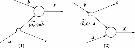
Kinematics of a single channel with one CS splitting
This is, of course, not true for other processes.
Rules for emissions from the second incoming line are analogous.
We employ here and in the following a shorthand notation \(\delta _{x=y}\equiv \delta (x-y)\).
The analysis in Ref. [1] for the DIS process, albeit limited to the gluonstrahlung NLO subprocess, gives hope for a possible positive answer.
Let us note that a similar reweighting method for real-parton radiation in the DY process was implemented some time ago in the PYTHIA PSMC algorithm in the so-called matrix-element correction mode [22]. However, it did not include the virtual NLO corrections and did not use the MC factorisation scheme, as it is in the case of the KrkNLO method.

References
S. Jadach, A. Kusina, W. Płaczek, M. Skrzypek, M. Slawinska, Phys. Rev. D 87, 034029 (2013). arXiv:1103.5015
S. Jadach, W. Płaczek, S. Sapeta, A. Siódmok, M. Skrzypek, JHEP 10, 052 (2015). arXiv:1503.06849
T. Gleisberg et al., JHEP 02, 007 (2009). arXiv:0811.4622
M. Bahr, S. Gieseke, M. Gigg, D. Grellscheid, K. Hamilton et al., Eur. Phys. J. C 58, 639–707 (2008). arXiv:0803.0883
J. Bellm, S. Gieseke, D. Grellscheid, A. Papaefstathiou, S. Platzer, et al., arXiv:1310.6877
S. Gieseke, C. Rohr, A. Siodmok, Eur. Phys. J. C 72, 2225 (2012). arXiv:1206.0041
S. Frixione, B.R. Webber, JHEP 06, 029 (2002). arXiv:hep-ph/0204244
P. Nason, JHEP 11, 040 (2004). arXiv:hep-ph/0409146
S. Platzer, S. Gieseke, JHEP 1101, 024 (2011). arXiv:0909.5593
S. Schumann, F. Krauss, JHEP 0803, 038 (2008). arXiv:0709.1027
S. Hoeche, S. Prestel, Eur. Phys. J. C 75(9), 461 (2015). arXiv:1506.05057
N. Fischer, S. Prestel, M. Ritzmann, P. Skands, arXiv:1605.06142
Z. Nagy, D.E. Soper, JHEP 1406, 097 (2014). arXiv:1401.6364
S. Catani, M.H. Seymour, Nucl. Phys. B 485, 291–419 (1997). arXiv:hep-ph/9605323
J.M. Campbell, R.K. Ellis, Phys. Rev. D 60, 113006 (1999). http://mcfm.fnal.gov. arXiv:hep-ph/9905386
K. Hamilton, P. Richardson, J. Tully, JHEP 04, 116 (2009). arXiv:0903.4345
A. Djouadi, M. Spira, P.M. Zerwas, Phys. Lett. B 264, 440–446 (1991)
G. Altarelli, R.K. Ellis, G. Martinelli, Nucl. Phys. B 157, 461 (1979)
S. Platzer, S. Gieseke, Eur. Phys. J. C 72, 2187 (2012). arXiv:1109.6256
J. Bellm et al., Eur. Phys. J. C 76(4), 196 (2016). arXiv:1512.01178
J. Bellm, G. Nail, S. Platzer, P. Schichtel, A. Siódmok, arXiv:1605.01338
G. Miu, T. Sjostrand, Phys. Lett. B 449, 313–320 (1999). arXiv:hep-ph/9812455
G. Altarelli, M.L. Mangano, Proccedings of the Workshop on Standard Model Physics (and More) at the LHC. Yellow Report, CERN 2000–04, 9 (2000)
A.D. Martin, W.J. Stirling, R.S. Thorne, G. Watt, Eur. Phys. J. C 63, 189–285 (2009). arXiv:0901.0002
S. Catani, M. Grazzini, Phys. Rev. Lett. 98, 222002 (2007). arXiv:hep-ph/0703012
M. Grazzini, JHEP 02, 043 (2008). arXiv:0801.3232
S. Jadach, G. Nail, W. Placzek, S. Sapeta, A. Siodmok, M. Skrzypek, arXiv:1607.06799
K. Hamilton, P. Nason, C. Oleari, G. Zanderighi, JHEP 1305, 082 (2013). arXiv:1212.4504
S. Hoeche, Y. Li, S. Prestel, arXiv:1405.3607
S. Alioli, C.W. Bauer, C. Berggren, F.J. Tackmann, J.R. Walsh, et al., JHEP 1406, 089 (2014). arXiv:1311.0286
S. Alioli, C.W. Bauer, C. Berggren, F.J. Tackmann, J.R. Walsh, Phys. Rev. D 92(9), 094020 (2015). arXiv:1508.01475
K. Hamilton, P. Nason, G. Zanderighi, JHEP 05, 140 (2015). arXiv:1501.04637
R. Frederix, K. Hamilton, JHEP 05, 042 (2016). arXiv:1512.02663
K. Hamilton, T. Melia, P.F. Monni, E. Re, G. Zanderighi, JHEP 09, 057 (2016). arXiv:1606.07062
Acknowledgements
We are grateful to Simon Platzer and Graeme Nail for the useful discussions and their help with the dipole parton shower implemented in Herwig 7. We are indebted to the Cloud Computing for Science and Economy project (CC1) at IFJ PAN (POIG 02.03.03-00-033/09-04) in Kraków whose resources were used to carry out some of the numerical computations for this project. We also thank Mariusz Witek and Miłosz Zdybał for their help with CC1. This work was funded in part by the MCnetITN FP7 Marie Curie Initial Training Network PITN-GA-2012-315877.
Author information
Authors and Affiliations
Corresponding author
Additional information
This work is partly supported by the Polish National Science Center Grant DEC-2011/03/B/ST2/02632 and the Polish National Science Centre Grant UMO-2012/04/M/ST2/00240.
Coefficient functions for DIS process in MC scheme
Coefficient functions for DIS process in MC scheme
The NLO coefficient functions \(C_2\) for deep-inelastic electron–proton scattering (DIS) in the \(\overline{\mathrm{MS}}\) factorisation scheme read
The corresponding coefficient functions in the MC factorisation scheme can be obtained from the above formulae with the help of the transformation-matrix elements \( K^\mathrm{MC}_{ij}\) in the following way:
These coefficient functions can be used in fitting the MC PDFs to experimental DIS data.
Rights and permissions
Open Access This article is distributed under the terms of the Creative Commons Attribution 4.0 International License (http://creativecommons.org/licenses/by/4.0/), which permits unrestricted use, distribution, and reproduction in any medium, provided you give appropriate credit to the original author(s) and the source, provide a link to the Creative Commons license, and indicate if changes were made.
Funded by SCOAP3
About this article

Cite this article
Jadach, S., Płaczek, W., Sapeta, S. et al. Parton distribution functions in Monte Carlo factorisation scheme. Eur. Phys. J. C 76, 649 (2016). https://doi.org/10.1140/epjc/s10052-016-4508-8
Received:
Accepted:
Published:
DOI: https://doi.org/10.1140/epjc/s10052-016-4508-8