
Abstract
Over the past decade, a large number of jet substructure observables have been proposed in the literature, and explored at the LHC experiments. Such observables attempt to utilize the internal structure of jets in order to distinguish those initiated by quarks, gluons, or by boosted heavy objects, such as top quarks and W bosons. This report, originating from and motivated by the BOOST2013 workshop, presents original particle-level studies that aim to improve our understanding of the relationships between jet substructure observables, their complementarity, and their dependence on the underlying jet properties, particularly the jet radius and jet transverse momentum. This is explored in the context of quark/gluon discrimination, boosted W boson tagging and boosted top quark tagging.
1 Introduction
The center-of-mass energies at the Large Hadron Collider are large compared to the heaviest of known particles, even after accounting for parton density functions. With the start of the second phase of operation in 2015, the center-of-mass energy will further increase from 7 TeV in 2010–2011 and 8 TeV in 2012 to 13 TeV. Thus, even the heaviest states in the Standard Model (and potentially previously unknown particles) will often be produced at the LHC with substantial boosts, leading to a collimation of the decay products. For fully hadronic decays, these heavy particles will not be reconstructed as several jets in the detector, but rather as a single hadronic jet with distinctive internal substructure. This realization has led to a new era of sophistication in our understanding of both standard Quantum Chromodynamics (QCD) jets, as well as jets containing the decay of a heavy particle, with an array of new jet observables and detection techniques introduced and studied to distinguish the two types of jets. To allow the efficient propagation of results from these studies of jet substructure, a series of BOOST Workshops have been held on an annual basis: SLAC (2009) [1], Oxford University (2010) [2], Princeton University (2011) [3], IFIC Valencia (2012) [4], University of Arizona (2013) [5], and, most recently, University College London (2014) [6]. Following each of these meetings, working groups have generated reports highlighting the most interesting new results, and often including original particle-level studies. Previous BOOST reports can be found at [7–9].
This report from BOOST 2013 thus views the study and implementation of jet substructure techniques as a fairly mature field, and focuses on the question of the correlations between the plethora of observables that have been developed and employed, and their dependence on the underlying jet parameters, especially the jet radius R and jet transverse momentum (\(p_{T} \)). In new analyses developed for the report, we investigate the separation of a quark signal from a gluon background (q / g tagging), a W signal from a gluon background (W-tagging) and a top signal from a mixed quark/gluon QCD background (top-tagging). In the case of top-tagging, we also investigate the performance of dedicated top-tagging algorithms, the HepTopTagger [10] and the Johns Hopkins Tagger [11]. We study the degree to which the discriminatory information provided by the observables and taggers overlaps by examining the extent to which the signal-background separation performance increases when two or more variables/taggers are combined in a multivariate analysis. Where possible, we provide a discussion of the physics behind the structure of the correlations and the \(p_{T} \) and R scaling that we observe.
We present the performance of observables in idealized simulations without pile-up and detector resolution effects; the relationship between substructure observables, their correlations, and how these depend on the jet radius R and jet \(p_{T} \) should not be too sensitive to such effects. Conducting studies using idealized simulations allows us to more clearly elucidate the underlying physics behind the observed performance, and also provides benchmarks for the development of techniques to mitigate pile-up and detector effects. A full study of the performance of pile-up and detector mitigation strategies is beyond the scope of the current report, and will be the focus of upcoming studies.
The report is organized as follows: in Sects. 2–4, we describe the methods used in carrying out our analysis, with a description of the Monte Carlo event sample generation in Sect. 2, the jet algorithms, observables and taggers investigated in our report in Sect. 3, and an overview of the multivariate techniques used to combine multiple observables into single discriminants in Sect. 4. Our results follow in Sects. 5–7, with q / g-tagging studies in Sect. 5, W-tagging studies in Sect. 6, and top-tagging studies in Sect. 7. Finally we offer some summary of the studies and general conclusions in Sect. 8.
The principal organizers of and contributors to the analyses presented in this report are: B. Cooper, S. D. Ellis, M. Freytsis, A. Hornig, A. Larkoski, D. Lopez Mateos, B. Shuve, and N. V. Tran.
2 Monte Carlo samples
Below, we describe the Monte Carlo samples used in the q/g tagging, W-tagging, and top-tagging sections of this report. Note that no pile-up (additional proton–proton interactions beyond the hard scatter) are included in any samples, and there is no attempt to emulate the degradation in angular and \(p_{T} \) resolution that would result when reconstructing the jets inside a real detector; such effects are deferred to future study.
2.1 Quark/gluon and W-tagging
Samples were generated at \(\sqrt{s} = 8 \,\mathrm{TeV}~\) for QCD dijets, and for \(W^+W^-\) pairs produced in the decay of a scalar resonance. The W bosons are decayed hadronically. The QCD events were split into subsamples of gg and \(q\bar{q}\) events, allowing for tests of discrimination of hadronic W bosons, quarks, and gluons.
Individual gg and \(q\bar{q}\) samples were produced at leading order (LO) using MadGraph5 [12], while \(W^+W^-\) samples were generated using the JHU Generator [13–15]. Both were generated using CTEQ6L1 PDFs [16]. The samples were produced in exclusive \(p_{T} \) bins of width 100 GeV, with the slicing parameter chosen to be the \(p_{T} \) of any final state parton or W at LO. At the parton level, the \(p_{T} \) bins investigated in this report were 300–400 GeV, 500–600 GeV and 1.0–1.1 TeV. The samples were then showered through Pythia8 (version 8.176) [17] using the default tune 4C [18]. For each of the various samples (\(W,\,q,\,g\)) and \(p_{T} \) bins, 500 k events were simulated.
2.2 Top-tagging
Samples were generated at \(\sqrt{s}=14\) TeV. Standard Model dijet and top pair samples were produced with Sherpa 2.0.0 [19–24], with matrix elements of up to two extra partons matched to the shower. The top samples included only hadronic decays and were generated in exclusive \(p_{T} \) bins of width 100 GeV, taking as slicing parameter the top quark \(p_{T} \). The QCD samples were generated with a lower cut on the leading parton-level jet \(p_{T} \), where parton-level jets are clustered with the anti-\(k_T\) algorithm and jet radii of \(R= 0.4,\,0.8,\,1.2\). The matching scale is selected to be \(Q_\mathrm{cut}=40,\,60,\,80\,\mathrm{GeV}\) for the \(p_{T\,\text {min}}=600, 1000\), and \(1500\,\mathrm{GeV}\) bins, respectively. For the top samples, 100k events were generated in each bin, while 200 k QCD events were generated in each bin.
3 Jet algorithms and substructure observables
In Sects. 3.1, 3.2, 3.3 and 3.4, we describe the various jet algorithms, groomers, taggers and other substructure variables used in these studies. Over the course of our study, we considered a larger set of observables, but for presentation purposes we included only a subset in the final analysis, eliminating redundant observables.
We organize the algorithms into four categories: clustering algorithms, grooming algorithms, tagging algorithms, and other substructure variables that incorporate information about the shape of radiation inside the jet. We note that this labelling is somewhat ambiguous: for example, some of the “grooming” algorithms (such as trimming and pruning) as well as N-subjettiness can be used in a “tagging” capacity. This ambiguity is particularly pronounced in multivariate analyses, such as the ones we present here, since a single variable can act in different roles depending on which other variables it is combined with. Therefore, the following classification is intended only to give an approximate organization of the variables, rather than as a definitive taxonomy.
Before describing the observables used in our analysis, we give our definition of jet constituents. As a starting point, we can think of the final state of an LHC collision event as being described by a list of “final state particles”. In the analyses of the simulated events described below (with no detector simulation), these particles include the sufficiently long lived protons, neutrons, photons, pions, electrons and muons with no requirements on \(p_{\mathrm {T}}\) or rapidity. Neutrinos are excluded from the jet analyses.
3.1 Jet clustering algorithms
Jet clustering Jets were clustered using sequential jet clustering algorithms [25] implemented in FastJet 3.0.3. Final state particles i, j are assigned a mutual distance \(d_{ij}\) and a distance to the beam, \(d_{i\mathrm {B}}\). The particle pair with smallest \(d_{ij}\) are recombined and the algorithm repeated until the smallest distance is from a particle i to the beam, \(d_{i\mathrm {B}}\), in which case i is set aside and labelled as a jet. The distance metrics are defined as
where \(\Delta R_{ij}^2=(\Delta \eta _{ij})^2+(\Delta \phi _{ij})^2\), with \(\Delta \eta _{ij}\) being the separation in pseudorapidity of particles i and j, and \(\Delta \phi _{ij}\) being the separation in azimuth. In this analysis, we use the anti-\(k_T\) algorithm (\(\gamma =-1\)) [26], the Cambridge/Aachen (C/A) algorithm (\(\gamma =0\)) [27, 28], and the \(k_T\) algorithm (\(\gamma =1\)) [29, 30], each of which has varying sensitivity to soft radiation in the definition of the jet.
This process of jet clustering serves to identify jets as (non-overlapping) sub-lists of final state particles within the original event-wide list. The particles on the sub-list corresponding to a specific jet are labeled the “constituents” of that jet, and most of the tools described here process this sub-list of jet constituents in some specific fashion to determine some property of that jet. The concept of constituents of a jet can be generalized to a more detector-centric version where the constituents are, for example, tracks and calorimeter cells, or to a perturbative QCD version where the constituents are partons (quarks and gluons). These different descriptions are not identical, but are closely related. We will focus on the MC based analysis of simulated events, while drawing insight from the perturbative QCD view. Note also that, when a detector (with a magnetic field) is included in the analysis, there will generally be a minimum \(p_{\mathrm {T}}\) requirement on the constituents so that realistic numbers of constituents will be smaller than, but presumably still proportional to, the numbers found in the analyses described here.
Qjets We also perform non-deterministic jet clustering [31, 32]. Instead of always clustering the particle pair with smallest distance \(d_{ij}\), the pair selected for combination is chosen probabilistically according to a measure
where \(d_\mathrm{min}\) is the minimum distance for the usual jet clustering algorithm at a particular step. This leads to a different cluster sequence for the jet each time the Qjet algorithm is used, and consequently different substructure properties. The parameter \(\alpha \) is called the rigidity and is used to control how sharply peaked the probability distribution is around the usual, deterministic value. The Qjets method uses statistical analysis of the resulting distributions to extract more information from the jet than can be found in the usual cluster sequence.
3.2 Jet grooming algorithms
Pruning Given a jet, re-cluster the constituents using the C/A algorithm. At each step, proceed with the merger as usual unless both
in which case the merger is vetoed and the softer branch discarded. The default parameters used for pruning [33] in this report are \(z_\mathrm{cut}=0.1\) and \(R_\mathrm{cut}=0.5\), unless otherwise stated. One advantage of pruning is that the thresholds used to veto soft, wide-angle radiation scale with the jet kinematics, and so the algorithm is expected to perform comparably over a wide range of momenta.
Trimming Given a jet, re-cluster the constituents into subjets of radius \(R_\mathrm{trim}\) with the \(k_T\) algorithm. Discard all subjets i with
The default parameters used for trimming [34] in this report are \(R_\mathrm{trim}=0.2\) and \(f_\mathrm{cut}=0.03\), unless otherwise stated.
Filtering Given a jet, re-cluster the constituents into subjets of radius \(R_\mathrm{filt}\) with the C/A algorithm. Re-define the jet to consist of only the hardest N subjets, where N is determined by the final state topology and is typically one more than the number of hard prongs in the resonance decay (to include the leading final-state gluon emission) [35]. While we do not independently use filtering, it is an important step of the HEPTopTagger to be defined later.
Soft drop Given a jet, re-cluster all of the constituents using the C/A algorithm. Iteratively undo the last stage of the C/A clustering from j into subjets \(j_1\), \(j_2\). If
discard the softer subjet and repeat. Otherwise, take j to be the final soft-drop jet [36]. Soft drop has two input parameters, the angular exponent \(\beta \) and the soft-drop scale \(z_\mathrm{cut}\). In these studies we use the default \(z_\mathrm{cut}=0.1\) setting, with \(\beta =2\).
3.3 Jet tagging algorithms
Modified mass drop tagger Given a jet, re-cluster all of the constituents using the C/A algorithm. Iteratively undo the last stage of the C/A clustering from j into subjets \(j_1\), \(j_2\) with \(m_{j_1}>m_{j_2}\). If either
then discard the branch with the smaller transverse mass \(m_T = \sqrt{m_i^2 + p_{Ti}^2}\), and re-define j as the branch with the larger transverse mass. Otherwise, the jet is tagged. If de-clustering continues until only one branch remains, the jet is considered to have failed the tagging criteria [37]. In this study we use by default \(\mu = 1.0\) (i.e. implement no mass drop criteria) and \(y_\mathrm{cut} = 0.1\). With respect to the singular parts of the splitting functions, this describes the same algorithm as running soft drop with \(\beta = 0\).
Johns Hopkins Tagger Re-cluster the jet using the C/A algorithm. The jet is iteratively de-clustered, and at each step the softer prong is discarded if its \(p_\mathrm{T}\) is less than \(\delta _p\,p_{\mathrm {T\,jet}}\). This continues until both prongs are harder than the \(p_\mathrm{T}\) threshold, both prongs are softer than the \(p_\mathrm{T}\) threshold, or if they are too close (\(|\Delta \eta _{ij}|+|\Delta \phi _{ij}|<\delta _R\)); the jet is rejected if either of the latter conditions apply. If both are harder than the \(p_\mathrm{T}\) threshold, the same procedure is applied to each: this results in 2, 3, or 4 subjets. If there exist 3 or 4 subjets, then the jet is accepted: the top candidate is the sum of the subjets, and W candidate is the pair of subjets closest to the W mass [11]. The output of the tagger is the mass of the top candidate (\(m_t\)), the mass of the W candidate (\(m_W\)), and \(\theta _\mathrm{h}\), a helicity angle defined as the angle, measured in the rest frame of the W candidate, between the top direction and one of the W decay products. The two free input parameters of the John Hopkins tagger in this study are \(\delta _p\) and \(\delta _R\), defined above, and their values are optimized for different jet kinematics and parameters in Sect. 7.
HEPTopTagger Re-cluster the jet using the C/A algorithm. The jet is iteratively de-clustered, and at each step the softer prong is discarded if \(m_1/m_{12}>\mu \) (there is not a significant mass drop). Otherwise, both prongs are kept. This continues until a prong has a mass \(m_i < m\), at which point it is added to the list of subjets. Filter the jet using \(R_\mathrm{filt}=\mathrm {min}(0.3,\Delta R_{ij})\), keeping the five hardest subjets (where \(\Delta R_{ij}\) is the distance between the two hardest subjets). Select the three subjets whose invariant mass is closest to \(m_t\) [10]. The top candidate is rejected if there are fewer than three subjets or if the top candidate mass exceeds 500 GeV. The output of the tagger is \(m_t\), \(m_W\), and \(\theta _\mathrm{h}\) (as defined in the Johns Hopkins Tagger). The two free input parameters of the HEPTopTagger in this study are m and \(\mu \), defined above, and their values are optimized for different jet kinematics and parameters in Sect. 7.
Top-tagging with pruning or trimming In the studies presented in Sect. 7 we add a W reconstruction step to the pruning and trimming algorithms, to enable a fairer comparison with the dedicated top tagging algorithms described above. Following the method of the BOOST 2011 report [8], a W candidate is found as follows: if there are two subjets, the highest-mass subjet is the W candidate (because the W prongs end up clustered in the same subjet), and the W candidate mass, \(m_W\), the mass of this subjet; if there are three subjets, the two subjets with the smallest invariant mass comprise the W candidate, and \(m_W\) is the invariant mass of this subjet pair. In the case of only one subjet, the top candidate is rejected. The top mass, \(m_t\), is the full mass of the groomed jet.
3.4 Other jet substructure observables
The jet substructure observables defined in this section are calculated using jet constituents prior to any grooming. This approach has been used in several analyses in the past, for example [38, 39], whilst others have used the approach of only considering the jet constituents that survive the grooming procedure [40]. We take the first approach throughout our analyses, as this approach allows a study of both the hard and soft radiation characteristic of signal vs. background. However, we do include the effects of initial state radiation and the underlying event, and unsurprisingly these can have a non-negligible effect on variable performance, particularly at large \(p_{T} \) and jet R. This suggests that the differences we see between variable performance at large \(p_{T}/R\) will be accentuated in a high pile-up environment, necessitating a dedicated study of pile-up to recover as much as possible the “ideal” performance seen here. Such a study is beyond the scope of this paper.
Qjet mass volatility As described above, Qjet algorithms re-cluster the same jet non-deterministically to obtain a collection of interpretations of the jet. For each jet interpretation, the pruned jet mass is computed with the default pruning parameters. The mass volatility, \(\Gamma _\mathrm{Qjet}\), is defined as [31]
where averages are computed over the Qjet interpretations. We use a rigidity parameter of \(\alpha =0.1\) (although other studies suggest a smaller value of \(\alpha \) may be optimal [31, 32]), and 25 trees per event for all of the studies presented here.
N -subjettiness N-subjettiness [41] quantifies how well the radiation in the jet is aligned along N directions. To compute N-subjettiness, \(\tau _N^{(\beta )}\), one must first identify N axes within the jet. Then,
where distances are between particles i in the jet and the axes,
and R is the jet clustering radius. The exponent \(\beta \) is a free parameter. There is also some choice in how the axes used to compute N-subjettiness are determined. The optimal configuration of axes is the one that minimizes N-subjettiness; recently, it was shown that the “winner-take-all” (WTA) axes can be easily computed and have superior performance compared to other minimization techniques [42]. We use both the WTA (Sect. 7) and one-pass \(k_T\) optimization axes (Sects. 5, 6) in our studies.
Often, a powerful discriminant is the ratio,
While this is not an infrared-collinear (IRC) safe observable, it is calculable [43] and can be made IRC safe with a loose lower cut on \(\tau _{N-1}\).
Energy correlation functions The transverse momentum version of the energy correlation functions are defined as [44]:
where i is a particle inside the jet. It is preferable to work in terms of dimensionless quantities, particularly the energy correlation function double ratio:
This observable measures higher-order radiation from leading-order substructure. Note that \(C_2^{\beta =0}\) is identical to the variable \(p_TD\) introduced by CMS in [45].
4 Multivariate analysis techniques
Multivariate techniques are used to combine multiple variables into a single discriminant in an optimal manner. The extent to which the discrimination power increases in a multivariable combination indicates to what extent the discriminatory information in the variables overlaps. There exist alternative strategies for studying correlations in discrimination power, such as “truth matching” [46], but these are not explored here.
In all cases, the multivariate technique used to combine variables is a Boosted Decision Tree (BDT) as implemented in the TMVA package [47]. An example of the BDT settings used in these studies, chosen to reduce the effect of overtraining, is given in [47]. The BDT implementation including gradient boost is used. Additionally, the simulated data were split into training and testing samples and comparisons of the BDT output were compared to ensure that the BDT performance was not affected by overtraining.
5 Quark–gluon discrimination
In this section, we examine the differences between quark- and gluon-initiated jets in terms of substructure variables. At a fundamental level, the primary difference between quark- and gluon-initiated jets is the color charge of the initiating parton, typically expressed in terms of the ratio of the corresponding Casimir factors \(C_F/C_A = 4/9\). Since the quark has the smaller color charge, it radiates less than a corresponding gluon and the naive expectation is that the resulting quark jet will contain fewer constituents than the corresponding gluon jet. The differing color structure of the two types of jet will also be realized in the detailed behavior of their radiation patterns. We determine the extent to which the substructure observables capturing these differences are correlated, providing some theoretical understanding of these variables and their performance. The motivation for these studies arises not only from the desire to “tag” a jet as originating from a quark or gluon, but also to improve our understanding of the quark and gluon components of the QCD backgrounds relative to boosted resonances. While recent studies have suggested that quark/gluon tagging efficiencies depend highly on the Monte Carlo generator used [48, 49], we are more interested in understanding the scaling performance with \(p_{T} \) and R, and the correlations between observables, which are expected to be treated consistently within a single shower scheme.
Other examples of recent analytic studies of the correlations between jet observables relevant to quark jet versus gluon jet discrimination can be found in [43, 46, 50, 51].
5.1 Methodology and observable classes
These studies use the qq and gg MC samples described in Sect. 2. The showered events were clustered with FastJet 3.03 using the anti-\(k_T\) algorithm with jet radii of \(R = 0.4,\, 0.8,\, 1.2\). In both signal (quark) and background (gluon) samples, an upper and lower cut on the leading jet \(p_{T} \) is applied after showering/clustering, to ensure similar \(p_{T} \) spectra for signal and background in each \(p_{T} \) bin. The bins in leading jet \(p_{T} \) that are considered are 300–400 GeV, 500–600 GeV, 1.0–1.1 TeV, for the 300–400 GeV, 500–600 GeV, 1.0–1.1 TeV parton \(p_{T} \) slices respectively. Various jet grooming approaches are applied to the jets, as described in Sect. 3.4. Only leading and subleading jets in each sample are used. The following observables are studied in this section:
-
Number of constituents (\(n_\mathrm{constits}\)) in the jet.
-
Pruned Qjet mass volatility, \(\Gamma _\mathrm{Qjet}\).
-
1-point energy correlation functions, \(C_1^{\beta }\) with \(\beta =0,\,1,\,2\).
-
1-subjettiness, \(\tau _1^{\beta }\) with \(\beta =1,\,2\). The N-subjettiness axes are computed using one-pass \(k_t\) axis optimization.
-
Ungroomed jet mass, m.
For simplicity, we hereafter refer to quark-initiated jets (gluon-initiated jets) as quark jets (gluon jets).
We will demonstrate that, in terms of their jet-by-jet correlations and their ability to separate quark jets from gluon jets, the above observables fall into five Classes. The first three observables, \(n_\mathrm{constits}\), \(\Gamma _\mathrm{Qjet}\) and \(C_1^{\beta =0}\), each constitutes a Class of its own (Classes I–III) in the sense that they each carry some independent information about a jet and, when combined, provide substantially better quark jet and gluon jet separation than any one observable alone. Of the remaining observables, \(C_1^{\beta =1}\) and \(\tau _1^{\beta =1}\) comprise a single class (Class IV) because their distributions are similar for a sample of jets, their jet-by-jet values are highly correlated, and they exhibit very similar power to separate quark jets and gluon jets (with very similar dependence on the jet parameters R and \(p_T\)); this separation power is not improved when they are combined. The fifth class (Class V) is composed of \(C_1^{\beta =2}\), \(\tau _1^{\beta =2}\) and the (ungroomed) jet mass. Again the jet-by-jet correlations are strong (even though the individual observable distributions are somewhat different), the quark versus gluon separation power is very similar (including the R and \(p_T\) dependence), and little is achieved by combining more than one of the Class V observables. This class structure is not surprising given that the observables within a class exhibit very similar dependence on the kinematics of the underlying jet constituents. For example, the members of Class V are constructed from of a sum over pairs of constituents using products of the energy of each member of the pair times the angular separation squared for the pair (this is apparent for the ungroomed mass when viewed in terms of a mass-squared with small angular separations). By the same argument, the Class IV and Class V observables will be seen to be more similar than any other pair of classes, differing only in the power (\(\beta \)) of the dependence on the angular separations, which produces small but detectable differences. We will return to a more complete discussion of jet masses in Sect. 5.4.
5.2 Single variable discrimination
In Fig. 1 are shown the quark and gluon distributions of different substructure observables in the \(p_{T} =500{-}600\,\mathrm{GeV}\) bin for \(R=0.8\) jets. These distributions illustrate some of the distinctions between the Classes made above. The fundamental difference between quarks and gluons, namely their color charge and consequent amount of radiation in the jet, is clearly indicated in Fig. 1a, suggesting that simply counting constituents provides good separation between quark and gluon jets. In fact, among the observables considered, one can see by eye that \(n_\mathrm{constits}\) should provide the highest separation power, i.e., the quark and gluon distributions are most distinct, as was originally noted in [49, 52]. Figure 1 further suggests that \(C_1^{\beta =0}\) should provide the next best separation, followed by \(C_1^{\beta =1}\), as was also found by the CMS and ATLAS Collaborations [48, 53].

Comparisons of quark and gluon distributions of different substructure variables, organized by Class, for leading jets in the \(p_{T} =500{-}600\,\mathrm{GeV}\) bin using the anti-\(k_T\) \(R=0.8\) algorithm. The first three plots are Classes I–III, with Class IV in the second row, and Class V in the third row

The ROC curve for all single variables considered for quark–gluon discrimination in the \(p_{T} \) 300–400 GeV bin using the anti-\(k_T\) \(R=0.4\) (top-left), 0.8 (top-right) and 1.2 (bottom) algorithm

Surface plots of \(1/\varepsilon _\text {bkg}\) for all single variables considered for quark–gluon discrimination as functions of R and \(p_{T} \). The first three plots are Classes I–III, with Class IV in the second row, and Class V in the third row
To more quantitatively study the power of each observable as a discriminator for quark/gluon tagging, Receiver Operating Characteristic (ROC) curves are built by scanning each distribution and plotting the background efficiency (to select gluon jets) vs. the signal efficiency (to select quark jets). Figure 2 shows these ROC curves for all of the substructure variables shown in Fig. 1 for \(R=0.4, 0.8\) and 1.2 jets (in the \(p_{T} =300\)–\(400\,\mathrm{GeV}\) bin). In addition, the ROC curve for a tagger built from a BDT combination of all the variables (see Sect. 4) is shown.
As suggested earlier, \(n_\mathrm{constits}\) is the best performing variable for all R values, although \(C_1^{\beta =0}\) is not far behind, particularly for \(R=0.8\). Most other variables have similar performance, with the main exception of \(\Gamma _\mathrm{Qjet}\), which shows significantly worse discrimination (this may be due to our choice of rigidity \(\alpha = 0.1\), with other studies suggesting that a smaller value, such as \(\alpha = 0.01\), produces better results [31, 32]). The combination of all variables shows somewhat better discrimination than any individual observable, and we give a more detailed discussion in Sect. 5.3 of the correlations between the observables and their impact on the combined discrimination power.
We now examine how the performance of the substructure observables varies with \(p_{T} \) and R. To present the results in a “digestible” fashion we focus on the gluon jet “rejection” factor, \(1/\varepsilon _\text {bkg}\), for a quark signal efficiency, \(\varepsilon _\text {sig}\), of \(50\,\%\). We can use the values of \(1/\varepsilon _\text {bkg}\) generated for the 9 kinematic points introduced above (\(R = 0.4, 0.8, 1.2\) and the 100 GeV \(p_{T} \) bins with lower limits \(p_T = 300\), 500, \(1000\,\text {GeV}\)) to generate surface plots. The surface plots in Fig. 3 indicate both the level of gluon rejection and the variation with \(p_{T} \) and R for each of the studied single observable. The color shading in these plots is defined so that a value of \(1/\varepsilon _\text {bkg}\simeq 1\) yields the color “violet”, while \(1/\varepsilon _\text {bkg}\simeq 20 \) yields the color “red”. The “rainbow” of colors in between vary linearly with \(\log _{10} (1/\varepsilon _\text {bkg})\).
We organize our results by the classes introduced in the previous subsection:
Class I The sole constituent of this class is \(n_\mathrm{constits}\). We see in Fig. 3a that, as expected, the numerically largest rejection rates occur for this observable, with the rejection factor ranging from 6 to 11 and varying rather dramatically with R. As R increases the jet collects more constituents from the underlying event, which are the same for quark and gluon jets, and the separation power decreases. At large R, there is some improvement with increasing \(p_{T} \) due to the enhanced QCD radiation, which is different for quarks vs. gluons.
Class II The variable \(\Gamma _\mathrm{Qjet}\) constitutes this class. Figure 3b confirms the limited efficacy of this single observable (at least for our parameter choices) with a rejection rate only in the range 2.5–2.8. On the other hand, this observable probes a very different property of jet substructure, i.e., the sensitivity to detailed changes in the grooming procedure, and this difference is suggested by the distinct R and \(p_{T} \) dependence illustrated in Fig. 3b. The rejection rate increases with increasing R and decreasing \(p_{T} \), since the distinction between quark and gluon jets for this observable arises from the relative importance of the one “hard” gluon emission configuration. The role of this contribution is enhanced for both decreasing \(p_{T} \) and increasing R. This general variation with \(p_{\mathrm {T}} \) and R is the opposite of what is exhibited in all of the other single variable plots in Fig. 3.
Class III The only member of this class is \(C_1^{\beta =0}\). Figure 3c indicates that this observable can itself provide a rejection rate in the range 7.8–8.6 (intermediate between the two previous observables), and again with distinct R and \(p_{T} \) dependence. In this case the rejection rate decreases slowly with increasing R, which follows from the fact that \(\beta = 0\) implies no weighting of \(\Delta R\) in the definition of \(C_1^{\beta =0}\), greatly reducing the angular dependence. The rejection rate peaks at intermediate \(p_{T} \) values, an effect visually enhanced by the limited number of \(p_{T} \) values included.
Class IV Figure 3d, e confirm the very similar properties of the observables \(C_1^{\beta =1}\) and \(\tau _1^{\beta =1}\) (as already suggested in Fig. 1d, e). They have essentially identical rejection rates (4.1–5.4) and identical R and \(p_{T} \) dependence (a slow decrease with increasing R and an even slower increase with increasing \(p_{T} \)).
Class V The observables \(C_1^{\beta =2}\), \(\tau _1^{\beta =2}\), and m have similar rejection rates in the range 3.5 to 5.3, as well as very similar R and \(p_{T} \) dependence (a slow decrease with increasing R and an even slower increase with increasing \(p_{T} \)).
Arguably, drawing a distinction between the Class IV and Class V observables is a fine point, but the color shading does suggest some distinction from the slightly smaller rejection rate in Class V. Again the strong similarities between the plots within the second and third rows in Fig. 3 speaks to the common properties of the observables within the two classes.
In summary, the overall discriminating power between quark and gluon jets tends to decrease with increasing R, except for the \(\Gamma _\mathrm{Qjet}\) observable, presumably in large part due to the contamination from the underlying event. Since the construction of the \(\Gamma _\mathrm{Qjet}\) observable explicitly involves pruning away the soft, large angle constituents, it is not surprising that it exhibits different R dependence. In general the discriminating power increases slowly and monotonically with \(p_{T} \) (except for the \(\Gamma _\mathrm{Qjet}\) and \(C_1^{\beta =0}\) observables). This is presumably due to the overall increase in radiation from high \(p_{T} \) objects, which accentuates the differences in the quark and gluon color charges and providing some increase in discrimination. In the following section, we study the effect of combining multiple observables.
5.3 Combined performance and correlations
Combining multiple observables in a BDT can give further improvement over cuts on a single variable. Since the improvement from combining correlated observables is expected to be inferior to that from combining uncorrelated observables, studying the performance of multivariable combinations gives insight into the correlations between substructure variables and the physical features allowing for quark/gluon discrimination. Based on our discussion of the correlated properties of observables within a single class, we expect little improvement in the rejection rate when combining observables from the same class, and substantial improvement when combining observables from different classes. Our classification of observables for quark/gluon tagging therefore motivates the study of particular combinations of variables for use in experimental analyses.
To quantitatively study the improvement obtained from multivariate analyses, we build quark/gluon taggers from every pair-wise combination of variables studied in the previous section; we also compare the pair-wise performance with the all-variables combination. To illustrate the results achieved in this way, we use the same 2D surface plots as in Fig. 3. Figure 4 shows pair-wise plots for variables in (a) Class IV and (b) Class V, respectively. Comparing to the corresponding plots in Fig. 3, we see that combining \(C_1^{\beta =1}+\tau _{1}^{\beta =1}\) provides a small (\(\sim \)10 %) improvement in the rejection rate with essentially no change in the R and \(p_{T} \) dependence, while combining \(C_1^{\beta =2}+\tau _{1}^{\beta =2}\) yields a rejection rate that is essentially identical to the single observable rejection rate for all R and \(p_{T} \) values (with a similar conclusion if one of these observables is replaced with the ungroomed jet mass m). This confirms the expectation that the observables within a single class effectively probe the same jet properties.
Next, we consider cross-class pairs of observables in Fig. 5, where, except in the one case noted below, we use only a single observable from each class for illustrative purposes. Since \(n_\mathrm{constits}\) is the best performing single variable, the largest rejection rates are obtained from combining another observable with \(n_ \mathrm{constits}\) (Fig. 5a–e). In general, the rejection rates are larger for the pair-wise case than for the single variable case. In particular, the pair \(n_\mathrm{constits}+ C_1^{\beta =1}\) in Fig. 5b yields rejection rates in the range 6.4–14.7 with the largest values at small R and large \(p_{T} \). As expected, the pair \(n_\mathrm{constits}+ \tau _1^{\beta =1}\) in Fig. 5e yields very similar rejection rates (6.4–15.0), since \(C_1^{\beta =1}\) and \(\tau _1^{\beta =1}\) are both in Class IV. The other pairings with \(n_\mathrm{constits}\) yield smaller rejection rates and smaller dynamic ranges. The pair \(n_ \mathrm{constits}+ C_1^{\beta =0}\) (Fig. 5d) exhibits the smallest range of rates (8.3–11.3), suggesting that the differences between these two observables serve to substantially reduce the R and \(p_{T} \) dependence for the pair. The other pairs shown exhibit similar behavior.

Surface plots of \(1/\varepsilon _{\text {bkg}}\) for the indicated pairs of variables from a Class IV and b Class V considered for quark–gluon discrimination as functions of R and \(p_{T} \)

Surface plots of \(1/\varepsilon _{\text {bkg}}\) for the indicated pairs of variables from different classes considered for quark–gluon discrimination as functions of R and \(p_{T} \)
The R and \(p_{T} \) dependence of the pair-wise combinations is generally similar to the single observable with the most dependence on R and \(p_{T} \). The smallest R and \(p_{T} \) variation always occurs when pairing with \(C_1^{\beta =0}\). Changing any of the observables in these pairs with a different observable in the same class (e.g., \(C_1^{\beta =2}\) for \(\tau _1^{\beta =2}\)) produces very similar results.
Figure 5l shows the performance of a BDT combination of all the current observables, with rejection rates in the range 10.5–17.1. The performance is very similar to that observed for the pair-wise \(n_\mathrm{constits}+ C_1^{\beta =1}\) and \(n_\mathrm{constits}+ \tau _1^{\beta =1}\) combinations, but with a somewhat narrower range and slightly larger maximum values. This suggests that almost all of the available information to discriminate quark and gluon-initiated jets is captured by \(n_\mathrm{constits}\) and \(C_1^{\beta =1}\) or \(\tau _1^{\beta =1}\) variables; this confirms the finding that near-optimal performance can be obtained with a pair of variables from [52].
Some features are more easily seen with an alternative presentation of the data. In Figs. 6 and 7 we fix R and \(p_{T} \) and simultaneously show the single- and pair-wise observables performance in a single matrix. The numbers in each cell are the same rejection rate for gluons used earlier, \(1/\varepsilon _\text {bkg}\), with \(\varepsilon _\text {sig}= 50\,\% \) (quarks). Figure 6 shows the results for \(p_{T} =1{-}1.1\) TeV and \(R =0.4,0.8,1.2\), while Fig. 7 is for \(R = 0.4\) and the 3 \(p_{T} \) bins. The single observable rejection rates appear on the diagonal, and the pairwise results are off the diagonal. The largest pair-wise rejection rate, as already suggested by Fig. 5e, appears at large \(p_{T} \) and small R for the pair \(n_ \mathrm{constits}+ \tau _1^{\beta =1}\) (with very similar results for \(n_ \mathrm{constits}+ C_1^{\beta =1}\)). The correlations indicated by the shadingFootnote 1 should be largely understood as indicating the organization of the observables into the now-familiar classes. The all-observable (BDT) result appears as the number at the lower right in each plot.
5.4 QCD jet masses
To close the discussion of q / g-tagging, we provide some insight into the behavior of the masses of QCD jets initiated by both kinds of partons, with and without grooming. Recall that, in practice, an identified jet is simply a list of constituents, i.e., final state particles. To the extent that the masses of these individual constituents can be neglected (due to the constituents being relativistic), each constituent has a “well- defined” 4-momentum from its energy and direction. It follows that the 4-momentum of the jet is simply the sum of the 4-momenta of the constituents and its square is the jet mass squared. Simply on dimensional grounds, we know that jet mass must have an overall linear scaling with \(p_{T} \), with the remaining \(p_{T} \) dependence arising predominantly from the running of the coupling, \(\alpha _s(p_{T})\). The R dependence is also crudely linear as the jet mass scales approximately with the largest angular opening between any 2 constituents, which is set by R.
To demonstrate this universal behavior for jet mass, we first note that if we consider the mass distributions for many kinematic points (various values of R and \(p_{T} \)), we observe considerable variation in behaviour. This variation, however, can largely be removed by plotting versus the scaled variable \(m/p_T/R\). The mass distributions for quark and gluon jets versus \(m/p_T/R\) for all of our kinematic points are shown in Fig. 8, where we use a logarithmic scale on the y-axis to clearly exhibit the behavior of these distributions over a large dynamic range. We observe that the distributions for the different kinematic points do approximately scale as expected, i.e., the simple arguments above capture most of the variation with R and \(p_{T} \). We will consider shortly an explanation of the residual non-scaling. A more rigorous quantitative understanding of jet mass distributions requires all-orders calculations in QCD, which have been performed for groomed and ungroomed jet mass spectra at high logarithmic accuracy, both in the context of direct QCD resummation [37, 54–56] and Soft Collinear Effective Theory [57–59].

Comparisons of quark and gluon ungroomed mass distributions versus the scaled variable \(m/p_T/R\)
Several features of Fig. 8 can be easily understood. The distributions all cut off rapidly for \(m/p_T/R > 0.5\), which is understood as the precise limit (maximum mass) for a jet composed of just two constituents. As expected from the soft and collinear singularities in QCD, the mass distribution peaks at small mass values. The actual peak is “pushed” away from the origin by the so-called Sudakov form factor. Summing the corresponding logarithmic structure (singular in both \(p_{T} \) and angle) to all orders in perturbation theory yields a distribution that is highly damped as the mass vanishes. In words, there is precisely zero probability that a color parton emits no radiation (and the resulting jet has zero mass). Above the Sudakov-suppressed part of phase space, there are two structures in the distribution: the “shoulder” and the “peak”. The large mass shoulder (\(0.3 < m/p_T/R < 0.5\)) is driven largely by the presence of a single large angle, energetic emission in the underlying QCD shower, i.e., this regime is quite well described by low-order perturbation theoryFootnote 2 In contrast, we can think of the peak region as corresponding to multiple soft emissions. This simple, necessarily approximate picture provides an understanding of the bulk of the differences between the quark and gluon jet mass distributions. Since the probability of the single large angle, energetic emission is proportional to the color charge, the gluon distribution should be enhanced in this region by a factor of about \(C_A/C_F = 9/4\), consistent with what is observed in Fig. 8. Similarly the exponent in the Sudakov damping factor for the gluon jet mass distribution is enhanced by the same factor, leading to a peak “pushed” further from the origin. Therefore, compared to a quark jet, the gluon jet mass distribution exhibits a larger average jet mass, with a larger relative contribution arising from the perturbative shoulder region and a small mass peak that is further from the origin.
Together with the fact that the number of constituents in the jet is also larger (on average) for the gluon jet simply because a gluon will radiate more than a quark, these features explain much of what we observed earlier in terms of the effectiveness of the various observables to separate quark jets from gluons jets. They also give us insight into the difference in the distributions for the observable \(\Gamma _\mathrm{Qjet}\). Since the shoulder is dominated by a single large angle, hard emission, it is minimally impacted by pruning, which is designed to remove the large angle, soft constituents (as shown in more detail below). Thus, jets in the shoulder exhibit small volatility and they are a larger component in the gluon jet distribution. Hence gluon jets, on average, have smaller values of \(\Gamma _\mathrm{Qjet}\) than quark jets as in Fig. 1b. Further, this feature of gluon jets is distinct from the fact that there are more constituents, explaining why \(\Gamma _\mathrm{Qjet}\) and \(n_ \mathrm{constits}\) supply largely independent information for distinguishing quark and gluon jets.
To illustrate some of these points in more detail, Fig. 9 exhibits the same jet mass distributions after pruning [33, 60]. Removing the large angle, soft constituents moves the peak in both of the distributions from \(m/p_T/R \sim 0.1 - 0.2\) to the region around \(m/p_T/R \sim 0.05\). This explains why pruning works to reduce the QCD background when looking for a signal in a specific jet mass bin. The shoulder feature at higher mass is much more apparent after pruning, as is the larger shoulder for the gluon jets. A quantitative (all-orders) understanding of groomed mass distributions is also possible. For instance, resummation of the pruned mass distribution was achieved in [37, 56]. Figure 9 serves to confirm the physical understanding of the relative behavior of \(\Gamma _\mathrm{Qjet}\) for quark and gluon jets.

Comparisons of quark and gluon pruned mass distributions versus the scaled variable \(m_\text {pr}/p_T/R\)
Our final topic in this section is the residual R and \(p_{T} \) dependence exhibited in Figs. 8 and 9, which indicates a deviation from the naive linear scaling that has been removed by using the scaled variable \(m/p_T/R\). A helpful, intuitively simple, if admittedly imprecise, model of a jet is to separate the constituents of the jet into “hard” (with \(p_{T} \)’s that are of order the jet \(p_{T} \)) versus “soft” (with \(p_{T} \)’s small and fixed compared to the jet \(p_{T} \)), and “large” angle (with an angular separation from the jet direction of order R) versus “small” angle (with an angular separation from the jet direction smaller than and not scaling with R) components. As described above the Sudakov damping factor excludes constituents that are very soft or very small angle (or both). In this simple picture perturbative large angle, hard constituents appear rarely, but, as described above, they characterize the large mass jets that appear in the “shoulder” of the jet mass distribution where the mass scales approximately linearly with the jet \(p_{T} \) and with R. The hard, small angle constituents are somewhat more numerous and contribute to a jet mass that does not scale with R. The soft constituents are much more numerous (becoming more numerous with increasing jet \(p_{T} \)) and contribute to a jet mass that scales like \(\sqrt{p_{T,\text {jet}}}\). The small angle, soft constituents contribute to a jet mass that does not scale with R, while the large angle, soft constituents do contribute to a jet mass that scales like R and grow in number approximately linearly in R (i.e., with the area of the annulus at the outer edge of the jet). This simple picture allows at least a qualitative explanation of the behavior observed in Figs. 8 and 9.
As already suggested, the residual \(p_{T} \) dependence can be understood as arising primarily from the slow decrease of the strong coupling \(\alpha _s(p_{T})\) as \(p_{T} \) increases. This leads to a corresponding decrease in the (largely perturbative) shoulder regime for both distributions at higher \(p_{T} \), i.e., a decrease in the number of hard, large angle constituents. At the same time, and for the same reason, the Sudakov damping is less strong with increasing \(p_{T} \) and the peak moves in towards the origin. While the number of soft constituents increases with increasing jet \(p_{T} \), their contributions to the scaled jet mass distribution shift to smaller values of \(m/p_{T} \) (decreasing approximately like \(1/\sqrt{p_{T}}\)). Thus the overall impact of increasing \(p_{T} \) for both distributions is a (gradual) shift to smaller values of \(m/p_T/R\). This is just what is observed in Figs. 8 and 9, although the numerical size of the effect is reduced in the pruned case.
The residual R dependence is somewhat more complicated. The perturbative large angle, hard constituent contribution largely scales in the variable \(m/p_T/R\), which is why we see little residual R dependence in either figure at higher masses (\(m/p_T/R > 0.4\)). The contribution of the small angle constituents (hard and soft) contribute at fixed m and thus shift to the left versus the scaled variable as R increases. This presumably explains the small shifts in this direction at small mass observed in both figures. The large angle, soft constituents contribute to mass values that scale like R, and, as noted above, tend to increase in number as R increases (i.e., as the area of the jet grows). Such contributions yield a scaled jet mass distribution that shifts to the right with increasing R and presumably explain the behavior at small \(p_{T} \) in Fig. 8. Since pruning largely removes this contribution, we observe no such behavior in Fig. 9.
5.5 Conclusions
In Sect. 5 we have seen that a variety of jet observables provide information about the jet that can be employed to effectively separate quark-initiated from gluon-initiated jets. Further, when used in combination, these observables can provide superior separation. Since the improvement depends on the correlation between observables, we use the multivariable performance to separate the observables into different classes, with each class containing highly correlated observables. We saw that the best performing single observable is simply the number of constituents in the jet, \(n_ \mathrm{constits}\), while the largest further improvement comes from combining with \(C_1^{\beta =1}\) (or \(\tau _1^{\beta =1}\)). The performance of this combined tagger is strongly dependent on \(p_{T} \) and R, with the best performance being observed for smaller R and higher \(p_{T} \). The smallest R and \(p_{T} \) dependence arises from combining \(n_ \mathrm{constits}\) with \(C_1^{\beta = 0}\). Some of the commonly used observables for q / g tagging are highly correlated and do not provide extra information when used together. We have found that adding further variables to the \(n_ \mathrm{constits}\) + \(C_1^{\beta =1}\) or \(n_ \mathrm{constits}\) + \(\tau _1^{\beta =1}\) BDT combination results in only a small improvement in performance, suggesting that almost all of the available information to discriminate quark and gluon-initiated jets is captured by \(n_\mathrm{constits}\) and \(C_1^{\beta =1}\) (or \(\tau _1^{\beta =1}\)) variables. In addition to demonstrating these correlations, we have provided a discussion of the physics behind the structure of the correlation. Using the jet mass as an example, we have given arguments to explicitly explain the differences between jet observables initiated by each type of parton.
Finally, we remind the reader that the numerical results were derived for a particular color configuration (qq and gg events), in a particular implementation of the parton shower and hadronization. Color connections in more complex event configurations, or different Monte Carlo programs, may well exhibit somewhat different efficiencies and rejection factors. The value of our results is that they indicate a subset of variables expected to be rich in information about the partonic origin of final-state jets. These variables can be expected to act as valuable discriminants in searches for new physics, and could also be used to define model-independent final-state measurements which would nevertheless be sensitive to the short-distance physics of quark and gluon production.
6 Boosted W-tagging
In this section, we study the discrimination of a boosted, hadronically decaying W boson (signal) against a gluon-initiated jet background, comparing the performance of various groomed jet masses and substructure variables. A range of different distance parameters for the anti-\(k_T\) jet algorithm are explored, in a range of different leading jet \(p_{T} \) bins. This allows us to determine the performance of observables as a function of jet radius and jet boost, and to see where different approaches may break down. The groomed mass and substructure variables are then combined in a BDT as described in Sect. 4, and the performance of the resulting BDT discriminant explored through ROC curves to understand the degree to which variables are correlated, and how this changes with jet boost and jet radius. Using BDT combinations of substructure variables to improve W tagging has been studied earlier in [61].
6.1 Methodology
These studies use the WW samples as signal and the dijet gg as background, described previously in Sect. 2. Whilst only gluonic backgrounds are explored here, the conclusions regarding the dependence of the performance and correlations on the jet boost and radius are not expected to be substantially different for quark backgrounds; we will see that the differences in the substructure properties of quark- and gluon-initiated jets, explored in the last section, are significantly smaller than the differences between W-initiated and gluon-initiated jets.
As in the q / g tagging studies, the showered events were clustered with FastJet 3.03 using the anti-\(k_T\) algorithm with jet radii of \(R = 0.4,\, 0.8,\, 1.2\). In both signal and background samples, an upper and lower cut on the leading jet \(p_{T} \) is applied after showering/clustering, to ensure similar \(p_{T} \) spectra for signal and background in each \(p_{T} \) bin. The bins in leading jet \(p_{T} \) that are considered are 300–400 GeV, 500–600 GeV, 1.0–1.1 TeV, for the 300–400 GeV, 500–600 GeV, 1.0–1.1 TeV parton \(p_{T} \) slices respectively. The jets then have various grooming algorithms applied and substructure observables reconstructed as described in Sect. 3.4. The substructure observables studied in this section are:
-
Ungroomed, trimmed (\(m_{\text {trim}}\)), and pruned (\(m_{\text {prun}}\)) jet masses.
-
Mass output from the modified mass drop tagger (\(m_{\text {mmdt}}\)).
-
Soft drop mass with \(\beta =2\) (\(m_{\mathrm {sd}}\)).
-
2-point energy correlation function ratio \(C_2^{\beta =1}\) (we also studied \(\beta =2\) but do not show its results because it showed poor discrimination power).
-
N-subjettiness ratio \(\tau _2 / \tau _1\) with \(\beta =1\) (\(\tau _{21}^{\beta =1}\)) and with axes computed using one-pass \(k_t\) axis optimization (we also studied \(\beta =2\) but did not show its results because it showed poor discrimination power).
-
Pruned Qjet mass volatility, \(\Gamma _\mathrm{Qjet}\).
6.2 Single variable performance
In this section we explore the performance of the various groomed jet mass and substructure variables in separating signal from background. Since we have not attempted to optimise the grooming parameter settings of each grooming algorithm, we do not place much emphasis here on the relative performance of the groomed masses, but instead concentrate on how their performance changes depending on the kinematic bin and jet radius considered.
Figure 10 compares the signal and background in terms of the different groomed masses explored for the anti-\(k_T\) \(R=0.8\) algorithm in the \(p_{T} \) = 500–600 GeV bin. One can clearly see that, in terms of separating signal and background, the groomed masses are significantly more performant than the ungroomed anti-\(k_T\) \(R=0.8\) mass. Using the same jet radius and \(p_{T} \) bin, Fig. 11 compares signal and background for the different substructure variables studied.
Figures 12, 13 and 14 show the single variable ROC curves for various \(p_{T} \) bins and values of R. The single variable performance is also compared to the ROC curve for a BDT combination of all the variables (labelled “allvars”). In all cases, the “allvars” option is significantly more performant than any of the individual single variables considered, indicating that there is considerable complementarity between the variables, and this is explored further in Sect. 6.3.
In Figs. 15, 16 and 17 the same information is shown in a format that more readily allows for a quantitative comparison of performance for different R and \(p_{T} \); matrices are presented which give the background rejection for a signal efficiency of 70 %Footnote 3 for single variable cuts, as well as two- and three-variable BDT combinations. The results are shown separately for each \(p_{T} \) bin and jet radius considered. Most relevant for our immediate discussion, the diagonal entries of these plots show the background rejections for a single variable BDT using the labelled observable, and can thus be examined to get a quantitative measure of the individual single variable performance, and to study how this changes with jet radius and momenta. The off-diagonal entries give the performance when two variables (shown on the x-axis and on the y-axis, respectively) are combined in a BDT. The final column of these plots shows the background rejection performance for three-variable BDT combinations of \(m_{sd}^{\beta =2} + C_2^{\beta =1} + X\). These results will be discussed later in Sect. 6.3.3.
In general, the most performant single variables are the groomed masses. However, in certain kinematic bins and for certain jet radii, \(C_2^{\beta =1}\) has a background rejection that is comparable to or better than the groomed masses.
We first examine the variation of performance with jet \(p_{T} \). By comparing Figs. 15a, 16a and 17b, we can see how the background rejection performance varies with increased momenta whilst keeping the jet radius fixed to \(R=0.8\). Similarly, by comparing Figs. 15b, 16b and 17c we can see how performance evolves with \(p_{T} \) for \(R=1.2\). For both \(R=0.8\) and \(R=1.2\) the background rejection power of the groomed masses increases with increasing \(p_{T} \), with a factor 1.5–2.5 increase in rejection in going from the 300–400 GeV to 1.0–1.1 TeV bins. In Fig. 18 we show the \(m_{\mathrm {sd}}\) and \(m_{\text {prun}}\) groomed masses for signal and background in the \(p_{T} \) = 300–400 and \(p_{T} \) = 1.0–1.1 TeV bins for \(R=1.2\) jets. Two effects result in the improved performance of the groomed mass at high \(p_{T} \). Firstly, as is evident from the figure, the resolution of the signal peak after grooming improves, because the groomer finds it easier to pick out the hard signal component of the jet against the softer components of the underlying event when the signal is boosted. Secondly, it follows from Fig. 9 and the discussion in Sect. 5.4 that, for increasing \(p_{T} \), the perturbative shoulder of the gluon distribution decreases in size, and thus there is a slight decrease (or at least no increase) of the background contamination in the signal mass region (m/\(p_{T}\)/R \(\sim \) 0.5).

The Soft-drop \(\beta =2\) and pruned groomed mass distribution for signal and background \(R=1.2\) jets in two different \(p_{T} \) bins
However, one can see from the Figs. 15b, 16b and 17c that the \(C_2^{\beta =1}\), \(\Gamma _\mathrm{Qjet}\) and \(\tau _{21}^{\beta =1}\) substructure variables behave somewhat differently. The background rejection power of the \(\Gamma _\mathrm{Qjet}\) and \(\tau _{21}^{\beta =1}\) variables both decrease with increasing \(p_{T} \), by up to a factor two in going from the 300–400 GeVto 1.0–1.1 TeV bins. Conversely the rejection power of \(C_2^{\beta =1}\) dramatically increases with increasing \(p_{T} \) for \(R=0.8\), but does not improve with \(p_{T} \) for the larger jet radius \(R=1.2\). In Fig. 19 we show the \(\tau _{21}^{\beta =1}\) and \(C_2^{\beta =1}\) distributions for signal and background in the \(p_{T} \) 300–400 GeV and \(p_{T} \) = 1.0–1.1 TeV bins for \(R=0.8\) jets. For \(\tau _{21}^{\beta =1}\) one can see that, in moving from lower to higher \(p_{T} \) bins, the signal peak remains fairly unchanged, whereas the background peak shifts to smaller \(\tau _{21}^{\beta =1}\) values, reducing the discriminating power of the variable. This is expected, since jet substructure methods explicitly relying on the identification of hard prongs would expect to work best at low \(p_{T} \), where the prongs would tend to be more separated. However, \(C_2^{\beta =1}\) does not rely on the explicit identification of subjets, and one can see from Fig. 19 that the discrimination power visibly increases with increasing \(p_{T} \). This is in line with the observation in [44] that \(C_2^{\beta =1}\) performs best when \(m/p_{T} \) is small. The negative correlation between the discrimination power of \(\Gamma _\mathrm{Qjet}\) and increasing \(p_{T} \) can be understood in similar terms. As discussed in Sect. 5.4, the low volatility component of a gluon jet, the “shoulder”, is enhanced as \(p_{T} \) increases leading to a background (QCD) volatility distribution more peaked at low values. In contrast the signal (W) jets will include more relatively soft radiation as \(p_{T} \) increases leading to a more volatile configuration. Thus, as \(p_{T} \) increases, the signal jets will exhibit a somewhat broader volatility distribution, while the background jets will exhibit a somewhat narrower volatility distribution, i.e., the distributions become more similar reducing the discriminating power of \(\Gamma _\mathrm{Qjet}\).

The \(\tau _{21}^{\beta =1}\) and \(C_2^{\beta =1}\) distributions for signal and background \(R=0.8\) jets in two different \(p_{T} \) bins
We now compare the performance of different jet radius parameters in the same \(p_{T} \) bin by comparing the individual sub-figures of Figs. 15, 16 and 17. To within \(\sim \)25 %, the background rejection power of the groomed masses remains constant with respect to the jet radius. Figure 20 shows how the groomed mass changes for varying jet radius in the \(p_{T} \) = 1.0–1.1 TeV bin. One can see that the signal mass peak remains unaffected by the increased radius, as expected, since grooming removes the soft contamination which could otherwise increase the mass of the jet as the radius increased. The gluon background in the signal mass region also remains largely unaffected, as follows from Fig. 9 and the discussion in Sect. 5.4, where it is shown that there is very little dependence of the groomed gluon mass distribution on R in the signal region (\(m/p_{T}/R \sim \) 0.5).

The soft-drop \(\beta =2\) and pruned groomed mass distribution for signal and background \(R=0.4\) and \(R=1.2\) jets in the \(p_{T} \) = 1.0–1.1 TeV bin
However, we again see rather different behaviour versus R for the substructure variables. In all \(p_{T} \) bins considered, the most performant substructure variable, \(C_2^{\beta =1}\), performs best for an anti-\(k_T\) distance parameter of \(R=0.8\). The performance of this variable is dramatically worse for the larger jet radius of \(R=1.2\) (a factor seven worse background rejection in the \(p_{T} \) = 1.0–1.1 TeV bin), and substantially worse for \(R=0.4\). For the other jet substructure variables considered, \(\Gamma _\mathrm{Qjet}\) and \(\tau _{21}^{\beta =1}\), their background rejection power also reduces for larger jet radius, but not to the same extent. Figure 21 shows the \(\tau _{21}^{\beta =1}\) and \(C_2^{\beta =1}\) distributions for signal and background in the \(p_{T} \) = 1.0–1.1 TeV bin for \(R=0.8\) and \(R=1.2\) jet radii. For the larger jet radius, the \(C_2^{\beta =1}\) distribution of both signal and background gets wider, and consequently the discrimination power decreases. For \(\tau _{21}^{\beta =1}\) there is comparatively little change in the distributions with increasing jet radius. The increased sensitivity of \(C_{2}\) to soft wide angle radiation in comparison to \(\tau _{21}\) is a known feature of this variable [44], and a useful feature in discriminating coloured versus colour singlet jets. However, at very large jet radii (\(R\sim 1.2\)), this feature becomes disadvantageous; the jet can pick up a significant amount of initial state or other uncorrelated radiation, and \(C_{2}\) is more sensitive to this than is \(\tau _{21}\). This uncorrelated radiation has no (or very little) dependence on whether the jet is W- or gluon-initiated, and so sensitivity to this radiation means that the discrimination power will decrease. A similar description applies to the variable \(\Gamma _\mathrm{Qjet}\), and the story is very similar to that for \(\Gamma _\mathrm{Qjet}\) with increasing \(p_{T} \). At larger R the low volatility “shoulder” is enhanced in the QCD background jet, leading to a narrower volatility distribution. For the W jet, the larger R includes more uncorrelated radiation in the jet, leading to a broader volatility distribution. So, as with increasing \(p_{T} \), increasing R results in volatility distributions for signal and background jets that are more similar and \(\Gamma _\mathrm{Qjet}\) exhibits reduced discrimination power.

The \(\tau _{21}^{\beta =1}\) and \(C_2^{\beta =1}\) distributions for signal and background \(R=0.8\) and \(R=1.2\) jets in the \(p_{T} \) = 1.0–1.1 TeV bin
6.3 Combined performance
Studying the improvement in performance (or lack thereof) when combining single variables into a multivariate analysis gives insight into the correlations among jet observables. The off-diagonal entries in Figs. 15, 16 and 17 can be used to compare the performance of different BDT two-variable combinations, and see how this varies as a function of \(p_{T} \) and R. By comparing the background rejection achieved for the two-variable combinations to the background rejection of the “all variables” BDT, one can also understand how discrimination can be improved by adding further variables to the two-variable BDTs.
In general the most powerful two-variable combinations involve a groomed mass and a non-mass substructure variable (\(C_2^{\beta =1}\), \(\Gamma _\mathrm{Qjet}\) or \(\tau _{21}^{\beta =1}\)). Two-variable combinations of the substructure variables are not as powerful in comparison. Which particular mass \(+\) substructure variable combination is the most powerful depends strongly on the \(p_{T} \) and R of the jet, as discussed in the sections to follow.
There is also modest improvement in the background rejection when different groomed masses are combined, indicating that there is complementary information between the different groomed masses (first shown in [62]). In addition, there is an improvement in the background rejection when the groomed masses are combined with the ungroomed mass, indicating that grooming removes some useful discriminatory information from the jet. These observations are explored further in the section below.
Generally, the \(R=0.8\) jets offer the best two-variable combined performance in all \(p_{T} \) bins explored here. This is despite the fact that in the highest \(p_{T} \) = 1.0–1.1 TeV bin the average separation of the quarks from the W decay is much smaller than 0.8, and well within 0.4. This conclusion could of course be susceptible to pile-up, which is not considered in this study. It is in marked contrast to the R dependence of the q / g tagging performance shown in Sect. 5, where a monotonic improvement in performance with reducing R is observed.
6.3.1 Mass + substructure performance
As already noted, the largest background rejection at 70 % signal efficiency are in general achieved using those two-variable BDT combinations which involve a groomed mass and a non-mass substructure variable. We now investigate the \(p_{T} \) and R dependence of the performance of these combinations.
For both \(R=0.8\) and \(R=1.2\) jets, the rejection power of these two-variable combinations increases substantially with increasing \(p_{T} \), at least within the \(p_{T} \) range considered here.
For a jet radius of \(R=0.8\), across the full \(p_{T} \) range considered, the groomed mass + substructure variable combinations with the largest background rejection are those which involve \(C_2^{\beta =1}\). For example, in combination with \(m_{\mathrm {sd}}\), this produces a 5-, 8- and 15-fold increase in background rejection compared to using the groomed mass alone. In Fig. 22 are shown 2-D histograms of \(m_{\mathrm {sd}}\) versus \(C_2^{\beta =1}\) for \(R=0.8\) jets in the various \(p_{T} \) bins considered, for both signal and background. The relatively low degree of correlation between \(m_{\mathrm {sd}}\) versus \(C_2^{\beta =1}\) that leads to these large improvements in background rejection can be seen. What little correlation exists is rather non-linear in nature, changing from a negative to a positive correlation as a function of the groomed mass, something which helps to improve the background rejection in the region of the W mass peak.

2-D histograms of \(m_{sd}^{\beta =2}\) versus \(C_2^{\beta =1}\) distributions for \(R=0.8\) jets in the various \(p_{T} \) bins considered, shown separately for signal and background

2-D histograms of \(m_{sd}^{\beta =2}\) versus \(C_2^{\beta =1}\) for \(R=0.4\), 0.8 and 1.2 jets in the \(p_{T} \) = 1.0–1.1 TeV bin, shown separately for signal and background

2-D histograms of \(m_{sd}^{\beta =2}\) versus \(\tau _{21}^{\beta =1}\) for \(R=0.4\), 0.8 and 1.2 jets in the \(p_{T} \) = 1.0–1.1 TeV bin, shown separately for signal and background
However, when we switch to a jet radius of \(R=1.2\) the picture for \(C_2^{\beta =1}\) combinations changes dramatically. These become significantly less powerful, and the most powerful variable in groomed mass combinations becomes \(\tau _{21}^{\beta =1}\) for all jet \(p_{T} \) considered. Figure 23 shows the correlation between \(m_{sd}^{\beta =2}\) and \(C_2^{\beta =1}\) in the \(p_{T} \) = 1.0–1.1 TeV bin for the various jet radii considered. Figure 24 is the equivalent set of distributions for \(m_{sd}^{\beta =2}\) and \(\tau _{21}^{\beta =1}\). One can see from Fig. 23 that, due to the sensitivity of the observable to soft, wide-angle radiation, as the jet radius increases \(C_2^{\beta =1}\) increases and becomes more and more smeared out for both signal and background, leading to worse discrimination power. This does not happen to the same extent for \(\tau _{21}^{\beta =1}\). We can see from Fig. 24 that the negative correlation between \(m_{sd}^{\beta =2}\) and \(\tau _{21}^{\beta =1}\) that is clearly visible for \(R=0.4\) decreases for larger jet radius, such that the groomed mass and substructure variable are far less correlated and \(\tau _{21}^{\beta =1}\) offers improved discrimination within a \(m_{sd}^{\beta =2}\) mass window.
6.3.2 Mass + mass performance
The different groomed masses and the ungroomed mass are of course not fully correlated, and thus one can always see some kind of improvement in the background rejection when two different mass variables are combined in the BDT. However, in some cases the improvement can be dramatic, particularly at higher \(p_{T} \), and particularly for combinations with the ungroomed mass. For example, in Fig. 17 we can see that in the \(p_{T} \) =1.0–1.1 TeV bin, the combination of pruned mass with ungroomed mass produces a greater than eightfold improvement in the background rejection for \(R=0.4\) jets, a greater than fivefold improvement for \(R=0.8\) jets, and a factor \(\sim \)2 improvement for \(R=1.2\) jets. A similar behaviour can be seen for mMDT mass. In Figs. 25, 26 and 27, we show the 2-D correlation plots of the pruned mass versus the ungroomed mass separately for the WW signal and gg background samples in the \(p_{T} \) = 1.0–1.1 TeV bin, for the various jet radii considered. For comparison, the correlation of the trimmed mass with the ungroomed mass, a combination that does not improve on the single mass as dramatically, is shown. In all cases one can see that there is a much smaller degree of correlation between the pruned mass and the ungroomed mass in the backgrounds sample than for the trimmed mass and the ungroomed mass. This is most obvious in Fig. 25, where the high degree of correlation between the trimmed and ungroomed mass is expected, since with the parameters used (in particular \(R_\mathrm{trim} = 0.2\)) we cannot expect trimming to have a significant impact on an \(R=0.4\) jet. The reduced correlation with ungroomed mass for pruning in the background means that, once we have required that the pruned mass is consistent with a W (i.e. \(\sim \)80\({\,\mathrm{GeV}}\)), a relatively large difference between signal and background in the ungroomed mass still remains, and can be exploited to improve the background rejection further. In other words, many of the background events which pass the pruned mass requirement do so because they are shifted to lower mass (to be within a signal mass window) by the grooming, but these events still have the property that they look very much like background events before the grooming. A requirement on the groomed mass alone does not exploit this property. Of course, the impact of pile-up, not considered in this study, could limit the degree to which the ungroomed mass could be used to improve discrimination in this way.

2-D histograms of groomed mass versus ungroomed mass in the \(p_{T} \) = 1.0–1.1 TeV bin using the anti-\(k_T\) \(R=0.4\) algorithm, shown separately for signal and background

2-D histograms of groomed mass versus ungroomed mass in the \(p_{T} \) = 1.0–1.1 TeV bin using the anti-\(k_T\) \(R=0.8\) algorithm, shown separately for signal and background

2-D histograms of groomed mass versus ungroomed mass in the \(p_{T} \) = 1.0–1.1 TeV bin using the anti-\(k_T\) \(R=1.2\) algorithm, shown separately for signal and background
6.3.3 “All variables” performance
Figures 15, 16 and 17 report the background rejection achieved by a combination of all the variables considered into a single BDT discriminant. In all cases, the rejection power of this “all variables” BDT is significantly larger than the best two-variable combination. This indicates that, beyond the best two-variable combination, there is still significant complementary information available in the remaining observables to improve the discrimination of signal and background. How much complementary information is available appears to be \(p_{T} \) dependent. In the lower \(p_{T} \) = 300–400 and 500–600 GeV bins, the background rejection of the “all variables” combination is a factor \(\sim \)1.5 greater than the best two-variable combination, but in the highest \(p_{T} \) bin it is a factor \(\sim \)2.5 greater.
The final column in Figs. 15, 16 and 17 allows us to further explore the all variables performance relative to the pair-wise performance. It shows the background rejection for three-variable BDT combinations of \(m_\mathrm{sd}^{\beta =2} + C_2^{\beta =1} + X\), where X is the variable on the y-axis. For jets with \(R=0.4\) and \(R=0.8\), the combination \(m_\mathrm{sd}^{\beta =2} + C_2^{\beta =1}\) is (at least close to) the best performant two-variable combination in every \(p_{T} \) bin considered. For \(R=1.2\) this is not the case, as \(C_2^{\beta =1}\) is superseded by \(\tau _{21}^{\beta =1}\) in performance, as discussed earlier. Thus, in considering the three-variable combination results, it is simplest to focus on the \(R=0.4\) and \(R=0.8\) cases. Here we see that, for the lower \(p_{T} \) = 300–400 and 500–600 GeV bins, adding the third variable to the best two-variable combination brings us to within \(\sim \)15 % of the “all variables” background rejection. However, in the highest \(p_{T} \) = 1.0–1.1 TeV bin, whilst adding the third variable does improve the performance considerably, we are still \(\sim \)40 % from the observed “all variables” background rejection, and clearly adding a fourth or maybe even fifth variable would bring considerable gains. In terms of which variable offers the best improvement when added to the \(m_\mathrm{sd}^{\beta =2} + C_2^{\beta =1}\) combination, it is hard to see an obvious pattern; the best third variable changes depending on the \(p_{T} \) and R considered.
It appears that there is a rich and complex structure in terms of the degree to which the discriminatory information provided by the set of variables considered overlaps, with the degree of overlap apparently decreasing at higher \(p_{T} \). This suggests that in all \(p_{T} \) ranges, but especially at higher \(p_{T} \), there are substantial performance gains to be made by designing a more complex multivariate W tagger.
6.4 Conclusions
We have studied the performance, in terms of the separation of a hadronically decaying W boson from a gluon-initiated jet background, of a number of groomed jet masses, substructure variables, and BDT combinations of the above. We have used this to gain insight into how the discriminatory information contained in the variables overlaps, and how this complementarity between the variables changes with jet \(p_{T} \) and anti-\(k_T\) distance parameter R.
In terms of the performance of individual variables, we find that, in agreement with other studies [40], the groomed masses generally perform best, with a background rejection power that increases with larger \(p_{T} \), but which is more consistent with respect to changes in R. We have explained the dependence of the groomed mass performance on \(p_{T} \) and R using the understanding of the QCD mass distribution developed in Sect. 5.4. Conversely, the performance of other substructure variables, such as \(C_2^{\beta =1}\) and \(\tau _{21}^{\beta =1}\), is more susceptible to changes in radius, with background rejection power decreasing with increasing R. This is due to the inherent sensitivity of these observables to soft, wide angle radiation.
The best two-variable performance is obtained by combining a groomed mass with a substructure variable. Which particular substructure variable works best in combination strongly depends on \(p_{\mathrm {T}}\) and R. The variable \(C_2^{\beta =1}\) offers significant complementarity to groomed mass for the smaller values of R investigated (\(R=0.4\) and 0.8), owing to the small degree of correlation between the variables. However, the sensitivity of \(C_2^{\beta =1}\) to soft, wide-angle radiation leads to worse discrimination power at \(R=1.2\), where \(\tau _{21}^{\beta =1}\) performs better in combination. The best two-variable performance in each \(p_{T} \) bin examined is obtained for \(C_2^{\beta =1}\) in combination with a groomed mass, using \(R=0.8\), with a performance that is better at higher \(p_{T} \). Our studies also demonstrate the potential for enhancing discrimination by combining groomed and ungroomed mass information, although the use of ungroomed mass in this may be limited in practice by the presence of pile-up that is not considered in these studies.
By examining the performance of a BDT combination of all variables considered, it is clear that there are potentially substantial performance gains to be made by designing a more complex multivariate W tagger, especially at higher \(p_{T} \).
7 Top tagging
In this section, we investigate the identification of boosted top quarks using jet substructure. Boosted top quarks result in large-radius jets with complex substructure, containing a b-subjet and a boosted W. As a consequence of the many kinematic differences between top and QCD jets, top taggers are typically complex, with a couple of input parameters necessary for any given algorithm. We study the variation in performance of top tagging techniques with respect to jet \(p_{T} \) and R, re-optimizing the tagger inputs for each kinematic range and jet radius considered. We also investigate the effects of combining dedicated top tagging algorithms with other jet substructure variables, giving insight into the correlations among top-tagging variables.
7.1 Methodology
We use the top quark MC samples for each bin described in Sect. 2.2. The analysis relies on FastJet 3.0.3 for jet clustering and calculation of jet substructure variables. Jets are clustered using the anti-\(k_T\) algorithm, and only the leading jet is used in each analysis. To ensure similar \(p_{T} \) spectra in each bin an upper and lower \(p_{T} \) cut are applied to each sample after jet clustering. The bins in leading jet \(p_{T} \) for top tagging are 600–700 GeV, 1–1.1 TeV , and 1.5–1.6 TeV. Jets are clustered with radii \(R=0.4\), 0.8, and 1.2; \(R=0.4\) jets are only studied in the 1.5–1.6 TeV bin because the top decay products are all contained within an \(R=0.4\) jet for top quarks with this boost.
We study a number of top-tagging strategies, which can be divided into two distinct categories. In the first category are dedicated top-tagging algorithms, which aim to directly reconstruct the top and W candidates in the top decay. In particular, we study:
-
1.
HEPTopTagger
-
2.
Johns Hopkins Tagger (JH)
-
3.
Trimming with W-identification
-
4.
Pruning with W-identification
as described in Sect. 3.3. In the case of the HepTopTagger and JH tagger, the algorithms produce three output variables (\(m_{t}\), \(m_{W}\) and helicity angle) that can be used to discriminate top jets from QCD. The trimming and pruning algorithms as used here produce two outputs, \(m_{t}\) and \(m_{W}\). All of the above taggers and groomers incorporate a step to remove contributions from the underlying event and other soft radiation to the reconstructed \(m_{t}\) and \(m_{W}\), and also explicitly rejects jets that do not meet basic selection criteria, as explained in detail in Sect. 3.3.
In the second category are individual jet substructure variables that are sensitive to the radiation pattern within the jet, which we refer to as “jet-shape variables”. While the most sensitive top-tagging variables are typically sensitive to three-pronged radiation, we also consider variables sensitive to two-pronged radiation in the limit where the W is very boosted and its subjets overlap. The variables we consider are:
-
The ungroomed jet mass.
-
N-subjettiness ratios \(\tau _{21}^{\beta =1}\) and \(\tau _{32}^{\beta =1}\), using the “winner-takes-all” axes definition.
-
2-point energy correlation function ratios \(C_2^{\beta =1}\) and \(C_3^{\beta =1}\).
-
The pruned Qjet mass volatility, \(\Gamma _\mathrm{Qjet}\).
Several of these variables were also considered earlier for q / g-tagging and W-tagging.
To study the correlations amongst the above substructure variables and tagging algorithms, we combine the relevant tagger output variables and/or jet shapes into a BDTFootnote 4, as described in Sect. 4. Additionally, because each tagger has two input parameters, we scan over reasonable values of the input parameters to determine the optimal value that gives the largest background rejection for each top tagging signal efficiency. This allows a direct comparison of the optimized version of each tagger. The input parameter values scanned for the various algorithms are:
-
HEPTopTagger \(m\in [30,100]\) GeV, \(\mu \in [0.5,1]\)
-
JH Tagger \(\delta _p\in [0.02,0.15]\), \(\delta _R\in [0.07,0.2]\)
-
Trimming \(f_\mathrm{cut}\in [0.02,0.14]\), \(R_\mathrm{trim}\in [0.1,0.5]\)
-
Pruning \(z_\mathrm{cut}\in [0.02,0.14]\), \(R_\mathrm{cut}\in [0.1,0.6]\)
We also investigate the degradation in performance of the top-tagging variables when moving away from the optimal parameter choice.
7.2 Single variable performance
We begin by investigating the behaviour of individual jet substructure variables. Because of the rich, three-pronged structure of the top decay, it is expected that combinations of masses and jet shapes will far outperform single variables in identifying boosted tops. However, a study of the top-tagging performance of single variables facilitates a direct comparison with the W tagging results in Sect. 6, and also allows a straightforward examination of the performance of each variable for different \(p_{T} \) and jet radius.
Top-tagging performance is quantified using ROC curves. Figure 28 shows the ROC curves for each of the top-tagging variables, with the bare (ungroomed) jet mass also plotted for comparison. The jet-shape variables all perform substantially worse than ungroomed jet mass; this is in contrast with W tagging, for which several variables are competitive with or perform better than ungroomed jet mass (see, for example, Figs. 16a, 17a, b). To understand why this is the case, consider N-subjettiness: the W is two-pronged and the top is three-pronged, and so we expect \(\tau _{21}\) and \(\tau _{32}\) to be the best-performant N-subjettiness ratios, respectively. However, a cut selection small values of \(\tau _{21}\) necessarily selects for events with large \(\tau _1\), which is strongly correlated with jet mass, up to exponentially suppressed contributions. Therefore, \(\tau _{21}\) applied to W-tagging indirectly incorporates some information about the jet mass in addition to shape information. By contrast, \(\tau _{32}\) applied to top tagging does not include any information on the ungroomed jet mass information. This likely accounts for why, relative to a cut on ungroomed mass, \(\tau _{32}\) for top tagging performs substantially worse than \(\tau _{21}\) for W-tagging.

Comparison of single-variable top-tagging performance in the \(p_{T} = 1{-}1.1\) GeV bin using the anti-\(k_T\), R \(=\) 0.8 algorithm
Of the two top-tagging algorithms, it is apparent from Fig. 28 that the Johns Hopkins tagger out-performs the HEPTopTagger in terms of its background rejection at fixed signal efficiency for both the top and W candidate masses; this is expected, as the HEPTopTagger was designed to reconstruct moderate-\(p_{T} \) top jets in ttH events (for a proposed high-\(p_{T} \) variant of the HEPTopTagger, see [65]). In Fig. 29, we show the histograms for the top mass output from the JH and HEPTopTagger for different R in the \(p_{T} \) = 1.5–1.6 TeV bin, and in Fig. 30 for different \(p_{T} \) at \(R=0.8\), optimized at a signal efficiency of 30 %. A particular feature of the HepTopTagger algorithm is that, after the jet is filtered to select the five hardest subjets, the three subjets are chosen which most closely reconstruct the top mass. This requirement tends to shape a peak in the QCD background around \(m_t\) for the HEPTopTagger, as can be seen from Figs. 29d and 30d; this is the likely reason for the better performance of the JH tagger, which has no such requirement. This effect is more pronounced at higher \(p_{T} \) and larger jet radius (see Figs. 32, 35). It has been proposed [63, 64] that performance of the HEPTopTagger may be improved by changing the selection criteria and/or performing a multivariate analysis with other variables. For example, the three subjets reconstructing the top should be selected only among those sets that pass the W mass constraints, which reduces the shaping of the background. We indeed confirm below that combining the HEPTopTagger with other variables reduces the discrepancy between the JH and the HEPTopTagger, and a preliminary study indicates that the new ordering prescriptions makes the tagger performances more comparable.

Comparison of top mass reconstruction with the Johns Hopkins (JH), HEPTopTaggers (HEP), pruning, and trimming at different R using the anti-\(k_T\) algorithm in the \(p_{T} \) = 1.5–1.6 TeV bin. Each histogram is shown for the working point optimized for best performance with \(m_t\) in the 0.3–0.35 signal efficiency bin, and is normalized to the fraction of events passing the tagger. In this and subsequent plots, the HEPTopTagger distribution cuts off at 500 GeV because the tagger fails to tag jets with a larger mass

Comparison of top mass reconstruction with the Johns Hopkins (JH), HEPTopTaggers (HEP), pruning, and trimming at different \(p_{T} \) using the anti-\(k_T\) algorithm, \(R=0.8\). Each histogram is shown for the working point optimized for best performance with \(m_t\) in the 0.3–0.35 signal efficiency bin, and is normalized to the fraction of events passing the tagger
We also see in Fig. 28b that the top mass from the JH tagger and the HEPTopTagger has superior performance relative to either of the grooming algorithms; this is because the pruning and trimming algorithms do not have inherent W-identification steps and are not optimized for this purpose. Indeed, because of the lack of a W-identification step, grooming algorithms are forced to strike a balance between under-grooming the jet, which broadens the signal peak due to underlying event contamination and features a larger background rate, and over-grooming the jet, which occasionally throws out the b-jet and preserves only the W components inside the jet. We demonstrate this effect in Figs. 29 and 30, showing that with 30 % signal efficiency, the optimal performance of the tagger over-grooms a substantial fraction of the jets (\(\sim \)20–30 %), leading to a spurious second peak at \(m_{W}\). This effect is more pronounced at large R and \(p_{T} \), since more aggressive grooming is required in these limits to combat the increased contamination from underlying event and QCD radiation.
In Figs. 31 and 32 we directly compare ROC curves for jet-shape variable performance and top-mass performance, respectively, in three different \(p_{T} \) bins whilst keeping the jet radius fixed at \(R=0.8\). The input parameters of the taggers, groomers and shape variables are separately optimized in each \(p_{T} \) bin. One can see from Fig. 31 that the tagging performance of jet shapes do not change substantially with \(p_{T} \). The variables \(\tau _{32}^{\beta =1}\) and \(\Gamma _\mathrm{Qjet}\) have the most variation and tend to degrade with higher \(p_{T} \), as can be seen in Fig. 33. This was also observed in the W-tagging studies in Sect. 6, and makes sense, as higher-\(p_{T} \) QCD jets have more, harder emissions within the jet, giving rise to substructure that fakes the signal. For the variable \(\Gamma _\mathrm{Qjet}\) (again as discussed in Sect. 6) increasing \(p_{T} \) leads to QCD jets with a narrower volatility distribution due to the enhanced contribution of the “shoulder” region, while for the signal (top) jets the increased amount of soft radiation with increasing \(p_{T} \) results in a broader volatility distribution. This with increasing \(p_{T} \) the signal and background jets exhibit more similar volatility distributions, as we see explicitly in Fig. 33a, b. Thus \(\Gamma _\mathrm{Qjet}\) becomes less discriminant for top identification as \(p_{T} \) increases. By contrast, from Fig. 32 we can see that most of the top-mass variables have superior performance at higher \(p_{T} \), due to the radiation from the top quark becoming more collimated. The notable exception is the HEPTopTagger, which degrades at higher \(p_{T} \), likely in part due to the background-shaping effects studied above and which is at least partially mitigated by recent updates to the HEPTopTagger [63, 64].

Comparison of individual jet shape performance at different \(p_{T} \) using the anti-\(k_T\) \(R=0.8\) algorithm

Comparison of top mass performance of different taggers at different \(p_{T} \) using the anti-\(k_T\) R \(=\) 0.8 algorithm

Comparison of \(\Gamma _\mathrm{Qjet}\) and \(\tau _{32}^{\beta =1}\) at \(R=0.8\) and different values of the \(p_{T} \). These shape variables are the most sensitive to varying \(p_{T} \)
In Figs. 34 and 35 we directly compare ROC curves for jet-shape variable performance and top-mass performance, respectively, for three different jet radii within the \(p_{T} \) = 1.5–1.6 TeV bin. Again, the input parameters of the taggers, groomers and shape variables are separately optimized for each jet radius. We can see from these figures that most of the top-tagging variables, both shape and reconstructed top mass, perform best for smaller radius, as was generally observed in the case of W-tagging in Sect. 6. This is likely because, at such high \(p_{T} \), most of the radiation from the top quark is confined within \(R=0.4\), and having a larger jet radius makes the variable more susceptible to contamination from the underlying event and other uncorrelated radiation. In Fig. 36, we compare the individual top signal and QCD background distributions for each shape variable considered in the \(p_{T} \) = 1.5–1.6 TeV bin for the various jet radii. In Fig. 36a–h the distributions for both signal and background broaden with increasing R, degrading the discriminating power. For \(C_2^{\beta =1}\) and \(C_3^{\beta =1}\), the background distributions are shifted to larger values as well. For the variable \(\Gamma _\mathrm{Qjet}\), as already discussed for increasing \(p_{T} \) (and in Sect. 6) the behavior with increasing R is a bit more complicated, with the QCD jets becoming less volatile and the signal jets more volatile, i.e., the two volatility distributions become more similar as we move from Fig. 36i, j. So again the discriminating power decreases with increasing R. The main exception is for \(C_3^{\beta =1}\), which performs optimally at \(R=0.8\); in this case, the signal and background coincidentally happen to have the same distribution around \(R=0.4\), and so \(R=0.8\) gives better discrimination.

Comparison of individual jet shape performance at different R in the \(p_{T} \) = 1.5–1.6 TeV bin

Comparison of top mass performance of different taggers at different R in the \(p_{T} \) = 1.5–1.6 TeV bin

Comparison of various shape variables in the \(p_{T} \) = 1.5–1.6 TeV bin and different values of the anti-\(k_\mathrm{T}\) radius R
7.3 Performance of multivariable combinations
We now consider various BDT combinations of the single variables considered in the last section, using the techniques described in Sect. 4. In particular, we consider the performance of individual taggers such as the JH tagger and HEPTopTagger, which output information about the top and W candidate masses and the helicity angle; for each tagger, all three output variables are combined in a BDT. For trimming and pruning, the output candidate \(m_{W}\) and \(m_{t}\) are combined in a BDT. Finally, we consider the combination of the full set of outputs of each of the above taggers/groomers with the shape variables, as well also a combination of the outputs of the HEPTopTagger and JH tagger. This allows us to determine the degree of complementary information in taggers/groomers and shape variables, as well as between the top tagging algorithms themselves. For all variables with tuneable input parameters, we scan and optimize over realistic values of such parameters, as described in Sect. 7.1.
In Fig. 37, we directly compare the performance of the HEPTopTagger, the JH tagger, trimming, and pruning, in the \(p_{T} = 1{-}1.1\) TeV bin with \(R=0.8\), where both \(m_{t}\) and \(m_{W}\) are used in the groomers. Generally, we find that pruning, which does not naturally incorporate subjets into the algorithm, does not perform as well as the others. Interestingly, trimming, which does include a subjet-identification step, performs comparably to the standard HEPTopTagger over much of the range, possibly due to the background-shaping observed in Sect. 7.2, although this can change with recent proposed updates to the HEPTopTagger [63, 64]. By contrast, the JH tagger outperforms the other standard algorithms. To determine whether there is complementary information in the mass outputs from different top taggers, we also consider in Fig. 37a multivariable combination of all of the JH and HEPTopTagger outputs. The maximum efficiency of the combined JH and HEPTopTaggers is limited, as some fraction of signal events inevitably fails either one or other of the taggers. We do see a 20–50 % improvement in performance when combining all outputs, which suggests that the different algorithms used to identify the top and W for different taggers contains complementary information.
In Fig. 38 we present the results for multivariable combinations of the top tagger outputs with and without shape variables. We see that, for both the HEPTopTagger and the JH tagger, the shape variables contain additional information uncorrelated with the masses and helicity angle, and give on average a factor 2–3 improvement in signal discrimination. We see that, when combined with the tagger outputs, both the energy correlation functions \(C_2+C_3\) and the N-subjettiness ratios \(\tau _{21}+\tau _{32}\) give comparable performance, while \(\Gamma _\mathrm{Qjet}\) is slightly worse; this is unsurprising, as Qjets accesses shape information in a more indirect way from other shape variables. Combining all shape variables with a single top tagger provides even greater enhancement in discrimination power. We directly compare the performance of the JH and HEPTopTaggers in Fig. 38c. Combining the taggers with shape information nearly erases the difference between the tagging methods observed in Fig. 37; this indicates that combining the shape information with the HEPTopTagger identifies the differences between signal and background missed by the standard tagger alone. This also suggests that further improvement to discriminating power may be minimal, as various multivariable combinations converge to within a factor of 20 % or so.

The performance of the various taggers in the \(p_{T} = 1-1.1\) TeV bin using the anti-\(k_T\) R \(=\) 0.8 algorithm. For the groomers a BDT combination of the reconstructed \(m_{t}\) and \(m_{W}\) are used. Also shown is a multivariable combination of all of the JH and HEPTopTagger outputs. The ungroomed mass performance is shown for comparison

The performance of BDT combinations of the JH and HepTopTagger outputs with various shape variables in the \(p_{T} = 1-1.1\) TeV bin using the anti-\(k_T\) \(R=0.8\) algorithm. Taggers are combined with the following shape variables: \(\tau _{21}^{\beta =1}+\tau _{32}^{\beta =1}\), \(C_{2}^{\beta =1}+C_{3}^{\beta =1}\), \(\Gamma _\mathrm{Qjet}\), and all of the above (denoted “shape”)
In Fig. 39 we present the results for multivariable combinations of groomer outputs with and without shape variables. As with the tagging algorithms, combinations of groomers with shape variables improves their discriminating power; combinations with \(\tau _{32}+\tau _{21}\) perform comparably to those with \(C_3+C_2\), and both of these are superior to combinations with the mass volatility, \(\Gamma _\mathrm{Qjet}\). Substantial further improvement is possible by combining the groomers with all shape variables. Not surprisingly, the taggers that lag behind in performance enjoy the largest gain in signal-background discrimination with the addition of shape variables. Once again, in Fig. 39c, we find that the differences between pruning and trimming are erased when combined with shape information.
Finally, in Fig. 40, we compare the performance of each of the tagger/groomers when their outputs are combined with all of the shape variables considered. One can see that the discrepancies between the performance of the different taggers/groomers all but vanishes, suggesting perhaps that we are here utilising all available signal-background discrimination information, and that this is the optimal top tagging performance that could be achieved in these conditions.

The performance of the BDT combinations of the trimming and pruning outputs with various shape variables in the \(p_{T} = 1-1.1\) TeV bin using the anti-\(k_T\) \(R=0.8\) algorithm. Groomer mass outputs are combined with the following shape variables: \(\tau _{21}^{\beta =1}+\tau _{32}^{\beta =1}\), \(C_{2}^{\beta =1}+C_{3}^{\beta =1}\), \(\Gamma _\mathrm{Qjet}\), and all of the above (denoted “shape”)

Comparison of the performance of the BDT combinations of all the groomer/tagger outputs with all the available shape variables in the \(p_{T} = 1-1.1\) TeV bin using the anti-\(k_T\) R \(=\) 0.8 algorithm. Tagger/groomer outputs are combined with all of the following shape variables: \(\tau _{21}^{\beta =1}+\tau _{32}^{\beta =1}\), \(C_{2}^{\beta =1}+C_{3}^{\beta =1}\), \(\Gamma _\mathrm{Qjet}\)
Up to this point, we have considered only the combined multivariable performance in the \(p_{T} \) = 1.0–1.1 TeV bin with jet radius \(R=0.8\). We now compare the BDT combinations of tagger outputs, with and without shape variables, at different \(p_{T} \). The taggers are optimized over all input parameters for each choice of \(p_{T} \) and signal efficiency. As with the single-variable study, we consider anti-\(k_T\) jets clustered with \(R=0.8\) and compare the outcomes in the \(p_{T} \) = 500–600 GeV, \(p_{T} \) = 1–1.1 TeV, and \(p_{T} \) = 1.5–1.6 TeV bins. The comparison of the taggers/groomers is shown in Fig. 41. The behaviour with \(p_{T} \) is qualitatively similar to the behaviour of the \(m_{t}\) variable for each tagger/groomer shown in Fig. 32; this suggests that the \(p_{T} \) behaviour of the taggers is dominated by the top-mass reconstruction. As before, the standard HEPTopTagger performance degrades slightly with increased \(p_{T} \) due to the background shaping effect (which may be mitigated by recently proposed updates), while the JH tagger and groomers modestly improve in performance.
In Fig. 42, we show the \(p_{T} \)-dependence of BDT combinations of the JH tagger output combined with shape variables. In terms of \(p_{T} \) dependence, we find that the curves look nearly identical to Fig. 41b: the \(p_{T} \) dependence is again dominated by the top-mass reconstruction, and combining the tagger outputs with different shape variables does not substantially change this behavior. Although not shown here, the same behavior is observed for trimming and pruning. By contrast, the \(p_{T} \) dependence of the HEPTopTagger ROC curves, shown in Fig. 43, does change somewhat when combined with different shape variables; due to the suboptimal performance of the HEPTopTagger at high \(p_{T} \) in the conventional configuration, we find that combining the HEPTopTagger with \(C_3^{\beta =1}\), which in Fig. 31b is seen to have some modest improvement at high \(p_{T} \), can improve its performance. Combining the standard HEPTopTagger with multiple shape variables gives the maximum improvement in performance at high \(p_{T} \) relative to at low \(p_{T} \).

Comparison at different \(p_{T} \) of the performance of various top tagging/grooming algorithms using the anti-\(k_T\) \(R=0.8\) algorithm. For each tagger/groomer, all output variables are combined in a BDT

Comparison at different \(p_{T} \) of the performance of the JH tagger using the anti-\(k_T\) \(R=0.8\) algorithm, where all tagger output variables are combined in a BDT with various shape variables

Comparison at different \(p_{T} \) of the performance of the HEPTopTagger using the anti-\(k_T\) \(R=0.8\) algorithm, where all tagger output variables are combined in a BDT with various shape variables
In Fig. 44 we compare the BDT combinations of tagger outputs, with and without shape variables, at different jet radius R in the \(p_{T} \) = 1.5–1.6 TeV bin. The taggers are optimized over all input parameters for each choice of R and signal efficiency. We find that, for all taggers and groomers, the performance is always best at small R; the choice of R is sufficiently large to admit the full top quark decay at such high \(p_{T} \), but is small enough to suppress contamination from additional radiation. This is not altered when the taggers are combined with shape variables. For example, in Fig. 45 is shown the dependence on R of the JH tagger when combined with shape variables, where one can see that the R-dependence is identical for all combinations. The same holds true for the HEPTopTagger, trimming, and pruning.

Comparison at different radii of the performance of various top tagging/grooming algorithms with \(p_{T} \) = 1.5–1.6 TeV. For each tagger/groomer, all output variables are combined in a BDT

Comparison at different radii of the performance of the JH tagger in the \(p_{T} \) = 1.5–1.6 TeV bin, where all tagger output variables are combined in a BDT with various shape variables
7.4 Performance at sub-optimal working points
Up until now, we have re-optimized our tagger and groomer parameters for each \(p_{T} \), R, and signal efficiency working point. In reality, experiments will choose a finite set of working points to use. When this is taken into account, how will the top-tagging performance compare to the optimal results already shown? To address this concern, we replicate our analyses, but optimize the top taggers only for a single \(p_{T} \) bin, single jet radius R, or single signal efficiency, and subsequently apply the same parameters to other scenarios. This allows us to determine the extent to which re-optimization is necessary to maintain the high signal-to-background discrimination power seen in the top-tagging algorithms we studied. In this section, we focus on the taggers and groomers, and their combination with shape variables, as the shape variables alone typically do not have any input parameters to optimize.
Optimizing at a single \(p_{T} \): We show in Fig. 46 the performance of the reconstructed top mass for the \(p_{T} \) = 0.6–0.7 TeV and \(p_{T} \) = 1.0–1.1 TeV bins, with all input parameters optimized to the \(p_{T} \) = 1.5–1.6 TeV bin (and \(R=0.8\) throughout). This is normalized to the performance using the optimized tagger inputs at each \(p_{T} \). The performance degradation is at the level of 20–30 % (at maximum 50 %) when the high-\(p_{T} \) optimized inputs are used at other momenta, with trimming and the Johns Hopkins tagger degrading the most. The jagged behaviour of the points is due to the finite resolution of the scan. We also observe a particular effect associated with using suboptimal taggers: since taggers sometimes fail to return a top candidate, parameters optimized for a particular signal efficiency \(\varepsilon _\mathrm{sig}\) at \(p_{T} \) = 1.5–1.6 TeV may not return enough signal candidates to reach the same efficiency at a different \(p_{T} \). Consequently, no point appears for that \(p_{T} \) value. This is not often a practical concern, as the largest gains in signal discrimination and significance are for smaller values of \(\varepsilon _\mathrm{sig}\), but it may be an important effect to consider when selecting benchmark tagger parameters and signal efficiencies.

Comparison of the top mass performance of different taggers at different \(p_{T} \) using the anti-\(k_T\) \(R=0.8\) algorithm. The tagger inputs are set to the optimum value for \(p_{T} \) = 1.5–1.6 TeV, and the performance is normalized to the performance using the optimized tagger inputs at each \(p_{T} \)
The degradation in performance is more pronounced for the BDT combinations of the full tagger outputs, shown in Fig. 47. This is true particularly at very low signal efficiency, where the optimization of inputs picks out a cut on the tail of some distribution that depends precisely on the \(p_{T} \)/R of the jet. Once again, trimming and the Johns Hopkins tagger degrade more markedly. Similar behavior holds for the BDT combinations of tagger outputs plus all shape variables.

Comparison of tagger performance at different \(p_{T} \) using the anti-\(k_T\) \(R=0.8\) algorithm. For each tagger/groomer, all output variables are combined in a BDT, and the tagger inputs are set to the optimum value for \(p_{T} \) = 1.5–1.6 TeV. The performance is normalized to the performance using the optimized tagger inputs at each \(p_{T} \)
Optimizing at a single R In Fig. 48, we show the performance of the reconstructed top mass for \(R=0.4\) and 0.8, with all input parameters optimized to \(R=1.2\) TeV bin (and \(p_{T} \) = 1.5–1.6 TeV throughout). This is normalized to the performance using the optimized tagger inputs at each R. While the performance of each variable degrades at small \(\varepsilon _\mathrm{sig}\) compared to the optimized search, the HEPTopTagger fares the worst. It is not surprising that a tagger whose top mass reconstruction is susceptible to background-shaping at large R and \(p_{T} \) would require a more careful optimization of parameters to obtain the best performance; recent updates to the tagger algorithm [63, 64] may mitigate the need for this more careful optimization.
The same holds true for the BDT combinations of the full tagger outputs, shown in Fig. 49. The performance for the sub-optimal taggers is still within an O(1) factor of the optimized performance, and the HEPTopTagger performs better with the combination of all of its outputs relative to the performance with just \(m_{t}\). The same behaviour holds for the BDT combinations of tagger outputs and shape variables.

Comparison of the top mass performance of different taggers at different R in the \(p_{T} \) = 1.5–1.6 TeV bin. The tagger inputs are set to the optimum value for \(R=1.2\), and the performance is normalized to the performance using the optimized tagger inputs at each R

Comparison of tagger performance at different R in \(p_{T} \) = 1.5–1.6 TeV bin. For each tagger/groomer, all output variables are combined in a BDT, and the tagger inputs are set to the optimum value for \(R=1.2\), and the performance is normalized to the performance using the optimized tagger inputs at each R
Optimizing at a single efficiency The strongest assumption we have made so far is that the taggers can be re-optimized for each signal efficiency point. This is useful for making a direct comparison of the power of different top-tagging algorithms, but is not particularly practical for LHC analyses. We now consider the scenario in which the tagger inputs are optimized once, in the \(\varepsilon _\mathrm{sig}=0.3\)–0.35 bin, and then used for all signal efficiencies. We do this in the \(p_{T} \) = 1.0–1.1 TeV bin and with \(R=0.8\).
The performance of each tagger, normalized to its performance optimized in each signal efficiency bin, is shown in Fig. 50 for cuts on the top mass and W mass, and in Fig. 51 for BDT combinations of tagger outputs and shape variables. In both plots, it is apparent that optimizing the taggers in the \(\varepsilon _\mathrm{sig}=0.3\)–0.35 efficiency bin gives comparable performance over efficiencies ranging from 0.2 to 0.5, although performance degrades at substantially different signal efficiencies. Pruning appears to give especially robust signal-background discrimination without re-optimization, most likely due to the fact that there are no absolute distance or \(p_{T} \) scales that appear in the algorithm. Figures 50 and 51 suggest that, while optimization at all signal efficiencies is a useful tool for comparing different algorithms, it is not crucial to achieve good top-tagging performance in experiments.
7.5 Conclusions
We have studied the performance of various jet substructure variables, groomed masses, and top taggers to study the performance of top tagging with different \(p_{T} \) and jet radius parameters. At each \(p_{T} \), R, and signal efficiency working point, we optimize the parameters for those variables with tuneable inputs. Overall, we have found that these techniques, individually and in combination, continue to perform well at high \(p_{T} \), at least at the particle-level, which is important for future LHC running. In general, the John Hopkins tagger performs best, while jet grooming algorithms under-perform relative to the best top taggers due to the lack of an optimized W-identification step. Tagger performance can be improved by a further factor of 2–4 through combination with jet substructure variables such as \(\tau _{32}\), \(C_3\), and \(\Gamma _\mathrm{Qjet}\). When combined with jet substructure variables, the performance of various groomers and taggers becomes very comparable, suggesting that, taken together, the variables studied are sensitive to nearly all of the physical differences between top and QCD jets at particle-level. A small improvement is also found by combining the Johns Hopkins and HEPTopTaggers, indicating that different taggers are not fully correlated. The degree to which these findings continue to hold under more realistic pile-up and detector configurations is, however, not addressed in this analysis and left to future study.
Comparing results at different \(p_{T} \) and R, top-tagging performance is generally better at smaller R due to less contamination from uncorrelated radiation. Similarly, most variables perform better at larger \(p_{T} \) due to the higher degree of collimation of radiation. Some variables fare worse at higher \(p_{T} \), such as the N-subjettiness ratio \(\tau _{32}\) and the Qjet mass volatility \(\Gamma _\mathrm{Qjet}\), as higher-\(p_{T} \) QCD jets have more and harder emissions that fake the top-jet substructure. The standard HEPTopTagger algorithm is also worse at high \(p_{T} \) due to the tendency of the tagger to shape backgrounds around the top mass. This is unsurprising, given that the HepTopTagger was specifically designed for a lower \(p_{\mathrm {T}}\) range than that considered here; recently proposed updates may improve performance at high \(p_{T} \) and R [63, 64]. The \(p_{T} \)- and R-dependence of the multivariable combinations is dominated by the \(p_{T} \)- and R-dependence of the top mass reconstruction component of the tagger/groomer.
Finally, we consider the performance of various tagger and jet substructure variable combinations under the more realistic assumption that the input parameters are only optimized at a single \(p_{T} \), R, or signal efficiency, and then the same inputs are used at other working points. Remarkably, the performance of all variables is typically within a factor of 2 of the fully optimized inputs, suggesting that while optimization can lead to substantial gains in performance, the general behavior found in the fully optimized analyses extends to more general applications of each variable. In particular, the performance of pruning typically varies the least when comparing sub-optimal working points to the fully optimized tagger due to the scale-invariant nature of the pruning algorithm.
8 Summary and conclusions
Furthering our understanding of jet substructure is crucial to enhancing the prospects for the discovery of new physical processes at Run II of the LHC. In this report we have studied the performance of jet substructure techniques over a wide range of kinematic regimes that will be encountered in Run II of the LHC. The performance of observables and their correlations have been studied by combining the variables into Boosted Decision Tree (BDT) discriminants, and comparing the background rejection power of this discriminant to the rejection power achieved by the individual variables. The performance of “all variables” BDT discriminants has also been investigated, to understand the potential of the “ultimate” tagger where “all” available particle-level information (at least, all of that provided by the variables considered) is used.

Comparison of top-tagging performance with \(m_{t}\) in the \(p_{T} = 1-1.1\) GeV bin using the anti-\(k_T\), \(R=0.8\) algorithm. The inputs for each tagger are optimized for the \(\varepsilon _\mathrm{sig}=0.3{-}0.35\) bin, and the performance is normalized to the performance using the optimized tagger inputs at each \(\varepsilon _\mathrm{sig}\)

The BDT combinations in the \(p_{T} = 1{-}1.1\) TeV bin using the anti-\(k_T\) \(R=0.8\) algorithm. Taggers are combined with the following shape variables: \(\tau _{21}^{\beta =1}+\tau _{32}^{\beta =1}\), \(C_{2}^{\beta =1}+C_{3}^{\beta =1}\), \(\Gamma _\mathrm{Qjet}\), and all of the above (denoted “shape”). The inputs for each tagger are optimized for the \(\varepsilon _\mathrm{sig}=0.3{-}0.35\) bin, and the performance is normalized to the performance using the optimized tagger inputs at each \(\varepsilon _\mathrm{sig}\)
We focused on the discrimination of quark jets from gluon jets, and the discrimination of boosted W bosons and top quarks from the QCD backgrounds. For each, we have identified the best-performing jet substructure observables at particle level, both individually and in combination with other observables. In doing so, we have also provided a physical picture of why certain sets of observables are (un)correlated. Additionally, we have investigated how the performance of jet substructure observables varies with R and \(p_{T} \), identifying observables that are particularly robust against or susceptible to these changes. In the case of q / g tagging, it seems that the ideal performance can be nearly achieved by combining the most powerful discriminant, the number of constituents of a jet, with just one other variable, \(C_1^{\beta =1}\) (or \(\tau _1^{\beta =1}\)). Many of the other variables considered are highly correlated and provide little additional discrimination. For both top and W tagging, the groomed mass is a very important discriminating variable, but one that can be substantially improved in combination with other variables. There is clearly a rich and complex relationship between the variables considered for W and top tagging, and the performance and correlations between these variables can change considerably with changing jet \(p_{T} \) and R. In the case of W tagging, even after combining groomed mass with two other substructure observables, we are still some way short of the ultimate tagger performance, indicating the complexity of the information available, and the complementarity between the observables considered. In the case of top tagging, we have shown that the performance of both the John Hopkins and HEPTopTagger can be improved when their outputs are combined with substructure observables such as \(\tau _{32}\) and \(C_{3}\), and that the performance of a discriminant built from groomed mass information plus substructure observables is very comparable to the performance of the taggers. We have optimized the top taggers for particular values of \(p_{T} \), R, and signal efficiency, and studied their performance at other working points. We have found that the performance of observables remains within at most a factor of two of the optimized value, suggesting that the performance of jet substructure observables is not significantly degraded when tagger parameters are only optimized for a few select benchmark points.
In all of q / g, W and top tagging, we have observed that the tagging performance improves with increasing \(p_{T} \). However, whereas for q / g and top tagging the performance improves with decreasing R (for the range of R considered here), the dependence on R for W tagging is more complex, with a peak performance at \(R=0.8\) for each \(p_{T} \) bin considered.
Our analyses were performed with ideal detector and pile-up conditions in order to most clearly elucidate the underlying physical scaling with \(p_{T} \) and R. At higher boosts, detector resolution effects will become more important, and with the higher pile-up expected at Run II of the LHC, pile-up mitigation will be crucial for future jet substructure studies. Future studies will be needed to determine which of the observables we have studied are most robust against pile-up and detector effects, and our analyses suggest particularly useful combinations of observables to consider in such studies.
At the new energy frontier of Run II of the LHC, boosted jet substructure techniques will be more central to our searches for new physics than ever before. By achieving a deeper understanding of the underlying structure of quark, gluon, W and top-initiated jets, as well as the relations between observables sensitive to their respective structures, it is hoped that more sophisticated analyses can be performed that will maximally extend the reach for new physics.
Notes
The connection between the value of the rejection rate and the shading color in Figs. 6 and 7 is the same as that in Figs. 3, 4 and 5.
Fig. 6 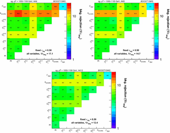
Gluon rejection defined as \(1/\varepsilon _\mathrm{gluon}\) when using each 2-variable combination as a tagger with 50 % acceptance for quark jets. Results are shown for jets with \(p_{T} =1{-}1.1\) TeV and for (top left) \(R=0.4\); (top right) \(R=0.8\); (bottom) \(R=1.2\). The rejection obtained with a tagger that uses all variables is also shown in the plots
Fig. 7 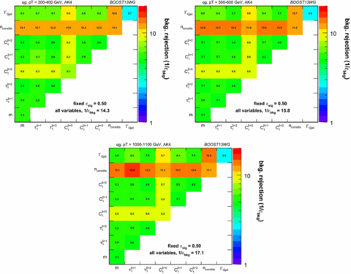
Gluon rejection defined as \(1/\varepsilon _\mathrm{gluon}\) when using each 2-variable combination as a tagger with 50 % acceptance for quark jets. Results are shown for \(\mathrm{R}=0.4\) jets with (top left) \(p_{T} =300{-}400\,\mathrm{GeV}\), (top right) \(p_{T} =500{-}600\,\mathrm{GeV}\) and (bottom) \(p_{T} =1{-}1.1\)TeV. The rejection obtained with a tagger that uses all variables is also shown in the plots
The shoulder label will become more clear when examining groomed jet mass distributions.
Note that we here choose to report the rejection for a higher signal efficiency than the 50 % that was used in the q / g tagging studies of Sect. 5, because the rejection rates in W tagging are considerably higher.
Fig. 10 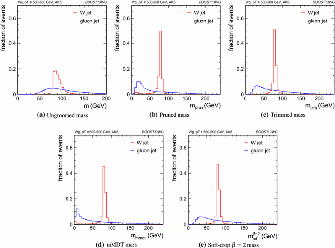
Leading jet mass distributions in the gg background and WW signal samples in the \(p_{T} \) = 500–600 GeV bin using the anti-\(k_T\) \(R=0.8\) algorithm
Fig. 11 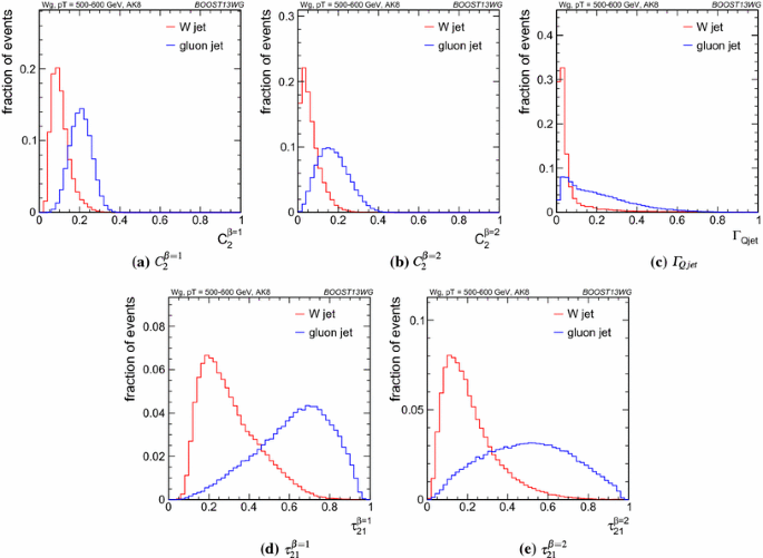
Leading jet substructure variable distributions in the gg background and WW signal samples in the \(p_{T} \) = 500–600 GeV bin using the anti-\(k_T\) \(R=0.8\) algorithm
Fig. 12 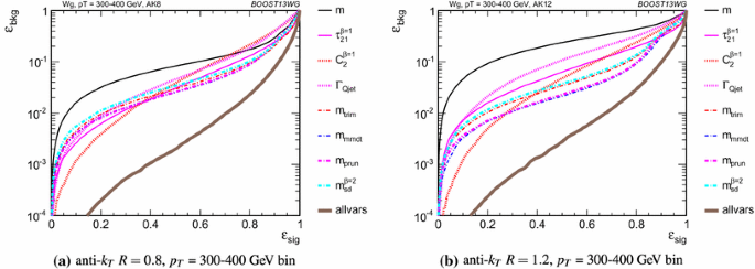
ROC curves for single variables considered for W tagging in the \(p_{T} \) = 300–400 GeV bin using the anti-\(k_T\) \(R=0.8\) algorithm and \(R=1.2\) algorithm, along with a BDT combination of all variables (“allvars”)
Fig. 13 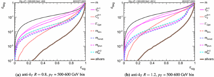
ROC curves for single variables considered for W tagging in the \(p_{T} \) = 500–600 GeV bin using the anti-\(k_T\) \(R=0.8\) algorithm and \(R=1.2\) algorithm, along with a BDT combination of all variables (“allvars”)
Fig. 14 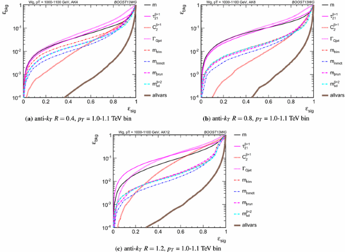
ROC curves for single variables considered for W tagging in the \(p_{T} \) = 1.0–1.1 TeV bin using the anti-\(k_T\) \(R=0.4\) algorithm, anti-\(k_T\) \(R=0.8\) algorithm and \(R=1.2\) algorithm, along with a BDT combination of all variables (“allvars”)
Fig. 15 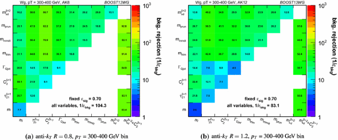
The background rejection for a fixed signal efficiency (70 %) of each BDT combination of each pair of variables considered, in the \(p_{T} \) = 300–400 GeV bin using the anti-\(k_T\) \(R=0.8\) algorithm and \(R=1.2\) algorithm. Also shown is the background rejection for three-variable combinations involving \(m_{sd}^{\beta =2} + C_2^{\beta =1}\), and for a BDT combination of all of the variables considered
Fig. 16 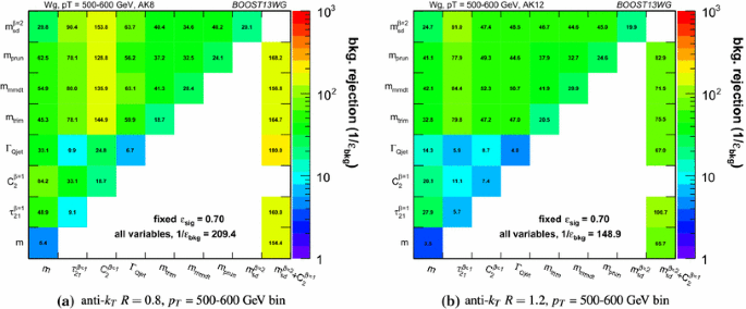
The background rejection for a fixed signal efficiency (70 %) of each BDT combination of each pair of variables considered, in the \(p_{T} \) = 500–600 GeV bin using the anti-\(k_T\) \(R=0.8\) algorithm and \(R=1.2\) algorithm. Also shown is the background rejection for three-variable combinations involving \(m_{sd}^{\beta =2} + C_2^{\beta =1}\), and for a BDT combination of all of the variables considered
Fig. 17 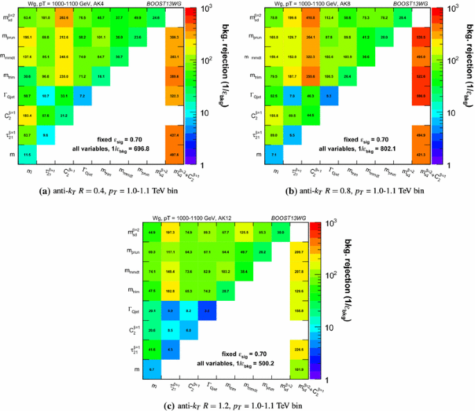
The background rejection for a fixed signal efficiency (70 %) of each BDT combination of each pair of variables considered, in the \(p_{T} \) = 1.0–1.1 TeV bin using the anti-\(k_T\) \(R=0.4\), \(R=0.8\) and \(R=1.2\) algorithm. Also shown is the background rejection for three-variable combinations involving \(m_{sd}^{\beta =2} + C_2^{\beta =1}\), and for a BDT combination of all of the variables considered


References
Boost, SLAC National Accelerator Laboratory, 9–10 July 2009 (2009). http://www-conf.slac.stanford.edu/Boost2009
Boost, University of Oxford, 22–25 June 2010 (2010). http://www.physics.ox.ac.uk/boost2010
Boost, Princeton University, 22–26 May 2011 (2011). https://indico.cern.ch/event/138809/
Boost, IFIC Valencia, 23–27 July 2012 (2012). http://ific.uv.es/boost2012
Boost, University of Arizona, 12–16 August 2013 (2013). https://indico.cern.ch/event/215704/
Boost, University College London, 18–22 August 2014 (2014). http://www.hep.ucl.ac.uk/boost2014/
A. Abdesselam, E.B. Kuutmann, U. Bitenc, G. Brooijmans, J. Butterworth, et al., Eur. Phys. J. C 71, 1661 (2011). doi:10.1140/epjc/s10052-011-1661-y
A. Altheimer, S. Arora, L. Asquith, G. Brooijmans, J. Butterworth, et al., J. Phys. G 39, 063001 (2012). doi:10.1088/0954-3899/39/6/063001
A. Altheimer, A. Arce, L. Asquith, J. Backus Mayes, E. Bergeaas Kuutmann, et al., Eur. Phys. J. C 74(3), 2792 (2014). doi:10.1140/epjc/s10052-014-2792-8
T. Plehn, M. Spannowsky, M. Takeuchi, D. Zerwas, JHEP 1010, 078 (2010). doi:10.1007/JHEP10(2010)078
D.E. Kaplan, K. Rehermann, M.D. Schwartz, B. Tweedie, Phys. Rev. Lett. 101, 142001 (2008). doi:10.1103/PhysRevLett.101.142001
J. Alwall, M. Herquet, F. Maltoni, O. Mattelaer, T. Stelzer, JHEP 1106, 128 (2011). doi:10.1007/JHEP06(2011)128
Y. Gao, A.V. Gritsan, Z. Guo, K. Melnikov, M. Schulze, et al., Phys. Rev. D 81, 075022 (2010). doi:10.1103/PhysRevD.81.075022
S. Bolognesi, Y. Gao, A.V. Gritsan, K. Melnikov, M. Schulze, et al., Phys. Rev. D 86, 095031 (2012). doi:10.1103/PhysRevD.86.095031
I. Anderson, S. Bolognesi, F. Caola, Y. Gao, A.V. Gritsan, et al., Phys. Rev. D 89, 035007 (2014). doi:10.1103/PhysRevD.89.035007
J. Pumplin, D. Stump, J. Huston, H. Lai, P.M. Nadolsky, et al., JHEP 0207, 012 (2002). doi:10.1088/1126-6708/2002/07/012
T. Sjostrand, S. Mrenna, P.Z. Skands, Comput. Phys. Commun. 178, 852 (2008). doi:10.1016/j.cpc.2008.01.036
A. Buckley, J. Butterworth, S. Gieseke, D. Grellscheid, S. Hoche, et al., Phys. Rept. 504, 145 (2011). doi:10.1016/j.physrep.2011.03.005
T. Gleisberg, S. Hoeche, F. Krauss, M. Schonherr, S. Schumann, et al., JHEP 0902, 007 (2009). doi:10.1088/1126-6708/2009/02/007
S. Schumann, F. Krauss, JHEP 0803, 038 (2008). doi:10.1088/1126-6708/2008/03/038
F. Krauss, R. Kuhn, G. Soff, JHEP 0202, 044 (2002). doi:10.1088/1126-6708/2002/02/044
T. Gleisberg, S. Hoeche, JHEP 0812, 039 (2008). doi:10.1088/1126-6708/2008/12/039
S. Hoeche, F. Krauss, S. Schumann, F. Siegert, JHEP 0905, 053 (2009). doi:10.1088/1126-6708/2009/05/053
M. Schonherr, F. Krauss, JHEP 0812, 018 (2008). doi:10.1088/1126-6708/2008/12/018
S. Bethke, et al., Phys. Lett. B 213, 235 (1988). doi:10.1016/0370-2693(88)91032-5
M. Cacciari, G.P. Salam, G. Soyez, JHEP 0804, 063 (2008). doi:10.1088/1126-6708/2008/04/063
Y.L. Dokshitzer, G. Leder, S. Moretti, B. Webber, JHEP 9708, 001 (1997). doi:10.1088/1126-6708/1997/08/001
M. Wobisch, T. Wengler, in Proceedings of the Monte Carlo Generators for HERA Physics Workshop, Hamburg, ed. by A. Doyle (1998)
S. Catani, Y.L. Dokshitzer, M. Seymour, B. Webber, Nucl. Phys. B 406, 187 (1993). doi:10.1016/0550-3213(93)90166-M
S.D. Ellis, D.E. Soper, Phys. Rev. D 48, 3160 (1993). doi:10.1103/PhysRevD.48.3160
S.D. Ellis, A. Hornig, T.S. Roy, D. Krohn, M.D. Schwartz, Phys. Rev. Lett. 108, 182003 (2012). doi:10.1103/PhysRevLett.108.182003
S.D. Ellis, A. Hornig, D. Krohn, T.S. Roy, JHEP 1501, 022 (2015). doi:10.1007/JHEP01(2015)022
S.D. Ellis, C.K. Vermilion, J.R. Walsh, Phys. Rev. D 81, 094023 (2010). doi:10.1103/PhysRevD.81.094023
D. Krohn, J. Thaler, L.T. Wang, JHEP, 084 (2010). doi:10.1007/JHEP02(2010)084
J.M. Butterworth, A.R. Davison, M. Rubin, G.P. Salam, Phys. Rev. Lett. 100, 242001 (2008). doi:10.1103/PhysRevLett.100.242001
A.J. Larkoski, S. Marzani, G. Soyez, J. Thaler, JHEP 1405, 146 (2014). doi:10.1007/JHEP05(2014)146
M. Dasgupta, A. Fregoso, S. Marzani, G.P. Salam, JHEP 1309, 029 (2013). doi:10.1007/JHEP09(2013)029
V. Khachatryan, et al., JHEP 1408, 173 (2014). doi:10.1007/JHEP08(2014)173
G. Aad, et al., New J. Phys. 16(11), 113013 (2014). doi:10.1088/1367-2630/16/11/113013
Performance of Boosted W Boson Identification with the ATLAS Detector. Tech. Rep. ATL-PHYS-PUB-2014-004, CERN, Geneva (2014)
J. Thaler, K. Van Tilburg, JHEP 1103, 015 (2011). doi:10.1007/JHEP03(2011)015
A.J. Larkoski, D. Neill, J. Thaler, JHEP 1404, 017 (2014). doi:10.1007/JHEP04(2014)017
A.J. Larkoski, J. Thaler, JHEP 1309, 137 (2013). doi:10.1007/JHEP09(2013)137
A.J. Larkoski, G.P. Salam, J. Thaler, JHEP 1306, 108 (2013). doi:10.1007/JHEP06(2013)108
S. Chatrchyan, et al., JHEP 1204, 036 (2012). doi:10.1007/JHEP04(2012)036
A.J. Larkoski, J. Thaler, W.J. Waalewijn, JHEP 1411, 129 (2014). doi:10.1007/JHEP11(2014)129
A. Hoecker, P. Speckmayer, J. Stelzer, J. Therhaag, E. von Toerne, H. Voss, An example of the BDT settings used in these studies are as follows: NTrees=1000; BoostType=Grad; Shrinkage=0.1; UseBaggedGrad=F; nCuts=10000; MaxDepth=3; UseYesNoLeaf=F; nEventsMin=200, PoS ACAT, 040 (2007)
G. Aad, et al., Eur. Phys. J. C 74(8), 3023 (2014). doi:10.1140/epjc/s10052-014-3023-z
J. Gallicchio, M.D. Schwartz, JHEP 1304, 090 (2013). doi:10.1007/JHEP04(2013)090
A.J. Larkoski, I. Moult, D. Neill, JHEP 1409, 046 (2014). doi:10.1007/JHEP09(2014)046
M. Procura, W.J. Waalewijn, L. Zeune, JHEP 1502, 117 (2015). doi:10.1007/JHEP02(2015)117
J. Gallicchio, M.D. Schwartz, Phys. Rev. Lett. 107, 172001 (2011). doi:10.1103/PhysRevLett.107.172001
C. Collaboration (2013)
H.n. Li, Z. Li, C.P. Yuan, Phys. Rev. D 87, 074025 (2013). doi:10.1103/PhysRevD.87.074025
M. Dasgupta, K. Khelifa-Kerfa, S. Marzani, M. Spannowsky, JHEP 1210, 126 (2012). doi:10.1007/JHEP10(2012)126
M. Dasgupta, A. Fregoso, S. Marzani, A. Powling, Eur. Phys. J. C 73(11), 2623 (2013). doi:10.1140/epjc/s10052-013-2623-3
Y.T. Chien, R. Kelley, M.D. Schwartz, H.X. Zhu, Phys. Rev. D 87(1), 014010 (2013). doi:10.1103/PhysRevD.87.014010
T.T. Jouttenus, I.W. Stewart, F.J. Tackmann, W.J. Waalewijn, Phys. Rev. D 88(5), 054031 (2013). doi:10.1103/PhysRevD.88.054031
Z.L. Liu, C.S. Li, J. Wang, Y. Wang, JHEP 1504, 005 (2015). doi:10.1007/JHEP04(2015)005
S.D. Ellis, C.K. Vermilion, J.R. Walsh, Phys. Rev. D 80, 051501 (2009). doi:10.1103/PhysRevD.80.051501
Y. Cui, Z. Han, M.D. Schwartz, Phys. Rev. D 83, 074023 (2011). doi:10.1103/PhysRevD.83.074023
D.E. Soper, M. Spannowsky, JHEP 1008, 029 (2010). doi:10.1007/JHEP08(2010)029
C. Anders, C. Bernaciak, G. Kasieczka, T. Plehn, T. Schell, Phys. Rev. D 89, 074047 (2014). doi:10.1103/PhysRevD.89.074047
G. Kasieczka, T. Plehn, T. Schell, T. Strebler, G.P. Salam (2015), JHEP 1506, 203 (2015). doi:10.1007/JHEP06(2015)203
S. Schaetzel, M. Spannowsky, Phys. Rev. D 89(1), 014007 (2014). doi:10.1103/PhysRevD.89.014007
Acknowledgments
We thank the Department of Physics at the University of Arizona for hosting and providing support for the BOOST 2013 workshop, and the US Department of Energy for their support of the workshop. We especially thank Vivian Knight (University of Arizona) for her help with the organization of the of the workshop. We also thank Prof. J. Boelts of the University of Arizona School of Art VisCom program and his Fall 2012 ART 465 class for organizing the design competition for the workshop poster. In particular, we thank the winner of the competition, Ms. Hallie Bolonkin, for creating the final design.
Author information
Authors and Affiliations
Corresponding author
Rights and permissions
Open Access This article is distributed under the terms of the Creative Commons Attribution 4.0 International License (http://creativecommons.org/licenses/by/4.0/), which permits unrestricted use, distribution, and reproduction in any medium, provided you give appropriate credit to the original author(s) and the source, provide a link to the Creative Commons license, and indicate if changes were made.
Funded by SCOAP3
About this article

Cite this article
Adams, D., Arce, A., Asquith, L. et al. Towards an understanding of the correlations in jet substructure. Eur. Phys. J. C 75, 409 (2015). https://doi.org/10.1140/epjc/s10052-015-3587-2
Received:
Accepted:
Published:
DOI: https://doi.org/10.1140/epjc/s10052-015-3587-2