
Abstract
Pulse compression technique plays a vital role in many communication systems e.g. optical, radio frequency (RF)/microwave, and biomedical applications. This article deals with demonstration of the technique in the atmospheric radar employed for wind profiling under various weather conditions. Relevant computation, simulations and analysis involved in practical application or implementation of this technique, that are achieved using the widely accepted complementary codes are presented. Moreover, making use of the computational and visualization features of MATLAB and LabVIEW packages, a flexible front-end graphic-user-interface (GUI) is designed and developed to demonstrate the functionality of this technique in the atmospheric radar operating at 206.5 MHz in the central Himalayan region. The GUI introduces the features of displaying coded or uncoded transmission and reception based on various user defined parameters such as pulse width (PW), pulse repetition frequency (PRF), Doppler frequency, and the number of data points. An interlock arrangement for inter-pulse period (IPP)—duty ratio is added to restrict the radar pulsed operation with the maximum duty ratio up to 15%. An arrangement is also made to visualize the auto and cross-correlations performed on the code sequences and RF signals. The user-friendly and easily customized GUI will benefit the larger user community in saving their time in writing their programs and/or constructing any hardware assemblies to test the performance of pulse compression technique during early design phases.
1 Introduction
Contemporary day communication systems relies on coding techniques for the intent of designing an efficient and reliable transmission system. Pulse compression is one such well-known coding technique being used in variety of applications, including the modern radio communication systems like radar and sonar, where propagation of radio wave or field through non-conducting medium such as air or space is involved [1,2,3,4,5,6]. The present article limits its investigation on the pulse compression application in radar used for profiling the atmosphere [7, 8].
Radar, an abbreviation for “Radio Detection and Ranging”, is a state-of-the-art technology for detecting the presence of target, determining their direction and range, and recognizing their character by means of radio waves [9]. The radar primarily used for the atmospheric probing and wind profiling are called atmospheric radar, which generally operates in pulsed mode, typically in the Very High Frequency (VHF) and Ultra High Frequency (UHF) bands, and basically works on the Doppler principle which was introduced by Austrian mathematician and physicist Christian Andreas Doppler in 18th century [10]. It is widely used to investigate structure and dynamics of the troposphere, stratosphere and mesosphere with unprecedented height and time resolutions [7, 8, 11,12,13]. The turbulent fluctuations in the refractive index of the atmosphere serve as target for these radars [8, 11]. Over the last few decades such radars have gained immense popularity in atmospheric research, but at the same time they pose challenges in retrieving the very weak back-scattered signals [8, 13, 14], and hence it is important to look into the signal processing aspects of such radars [15, 16], which is the subject of our interest here in this article.
An ideal pulsed radar transmits a short pulse of high magnitude, which is then detected by the receiver after some delay. The receiver may receive several smaller pulses reflected from different scattering points within the target. The interval between these smaller pulses defines the resolution (ΔR), which can be resolved before the reflection from two close scattering points. Usually the peak power from the transmitter is limited, and for its given value, the maximum range coverage (R) with desired signal-to-noise ratio (SNR) can be achieved by lengthening the pulse, i.e. sacrificing with ΔR [17]. For some problems, however both maximum R and smaller ΔR are needed, which in turn poses the requirement of impractical values of power from the transmitter, which are unacceptable in most systems. To circumvent such requirements, the pulse compression coding technique is used, in which the codes are superimposed onto the carrier wave. The technique allows radar to achieve data acquisition with maximum range coverage with smaller ΔR and high SNR, at reasonable power levels.
In this work, an attempt is made to demonstrate the usefulness of pulse compression technique in the context of atmospheric radars through GUI based approach that will save a lot of time spent on computer programming and/or constructing any hardware assemblies for testing and demonstration purposes. Apart from the design and development of the GUI tools using LabVIEW, the paper also discusses the salient results on pulse compression technique, obtained from numerical analysis and simulations performed in MATLAB. Section 2 describes the characteristics of the RF pulses, coding schemes, complementary codes, and their properties. Section 3 presents the simulation results and functions of different GUI panels. Section 4 covers the discussion, which is then followed by conclusion in Sect. 5.
2 Theoretical background
2.1 Pulsed waveform
Almost all the pulsed waveforms with constant amplitude and phase (or frequency) are in the form:
where \(u\left( t \right)\) is the pulsed signal, t is the time, e is the Euler’s constant used as base in logarithmic and exponential functions, j is the unit imaginary number that equals square root of − 1, \(\varphi \left( t \right) = \omega t + \phi\), the angular frequency \(\omega = 2\pi f\), \(f\) is the number of cycles per unit time, \(\phi\) is the phase, \(\tau_{p}\) is the PW, and \(rect\left[ {\frac{t}{{\tau_{p} }}} \right] = \left\{ {\begin{array}{*{20}c} {1, \quad 0 \le t \le \tau_{p} } \\ {0, \quad {\text{elsewhere}}} \\ \end{array} } \right.\)
The generation of pulse compression waveform in any radar application involves the two fundamental parameters of the RF waves:
-
Bandwidth The RF carrier will have a particular set of frequencies, with some minimum and maximum range. The total amount of frequency spectrum used by a channel is known as the RF bandwidth.
-
Modulation Carrier waves are generally sinusoidal in nature, defined by their properties of amplitude, frequency and phase. By varying one of these three properties in accordance with the instantaneous values of the modulating signal, they can carry information. This process is known as modulation.
In this work, the carrier frequency is chosen as 206.5 MHz with 5 MHz bandwidth. The atmospheric radar at this frequency has been installed at Aryabhatta Research Institute of observational sciencES (ARIES), Nainital, India which is one of the pristine sites (at 29.22° N, 79.28° E, ~ 1800 m above mean sea level) located in the central Himalayan region [18]. This is a monostatic, active, coherent, pulsed Doppler radar presently being used in obtaining the vertical profiles of wind and its three components namely the zonal (U), meridional (V) and vertical (W) wind up to the lower Stratospheric heights on a continuous basis, with good vertical and temporal resolutions.
2.2 Coding schemes
In the atmospheric radar application, two different types of binary phase codes are popular—Barker codes, and the complementary codes.
Barker codes have been used in the radars deployed for ionospheric incoherent scatter measurements, where the correlation time of the scattering medium is substantially longer than the full-uncompressed length of the transmitted pulse [19,20,21]. The decoding involves adding and subtracting the signal amplitude. If the scattering centers move a significant fraction of the radar’s wavelength between time of arrival of the first and last baud of the pulse, the compression process may fails. The Barker codes offer good pulse compression, and easy decoding, however, they suffers from fairly unacceptable side-lobe suppression. In addition, the Barker sequences are only available for the length of 2, 3, 4, 5, 7, 11 and 13 bauds (Table 1). Due to these limitations, they have limited utility in the atmospheric radar application.
The complementary codes are another form of the binary phase codes that come in pair [22]. They are decoded by matched filter/delay line combination whose impulse response is the time reverse of the pulse. The two pulses encoded with the complementary pair have the property that their side-lobes are equal in magnitude but opposite in sign, so when the outputs are added, the side-lobes cancel out, leaving only the central peak. As far as the complementary codes are concerned, there is still one main restriction i.e. the phase changes introduced by the target must vary only on a time scale much longer than the IPP. This restriction has prevented the use of this code in military applications and in incoherent scatter from ionosphere, where the Doppler shifts are too large. In comparison to the Barker codes, the implementation of pulse compression using complementary codes is quite suitable in atmospheric radar where the received backscattered signal have long correlation time and the Doppler shifts are quite small. For the 206.5 MHz atmospheric radar installed at ARIES, the use of complementary codes for pulse compression is entirely compatible. However, the selection of most suitable complementary code pairs must be decided based on several performance measures like merit factor, discrimination, quality factor, integrated side-lobe level (ISL) and peak side-lobe level (PSL), discussed elsewhere [23].
2.3 Complementary codes and their properties
Golay [22] defined a pair of complementary codes as two equally long finite sequences of two kinds of elements with the property that the number of pairs of like elements (L) with any given separation in one sequence is equal to the number of pairs of unlike elements (U) with the same separation in the other sequence. Figure 1 illustrates this property using 8-bit complementary pairs: A = {− 1, − 1, − 1, 1, − 1, − 1, 1, − 1} and B = {− 1, − 1, − 1, 1, 1, 1, − 1, 1}, where binary ‘1’ in the code sequence represents 0° in phase and binary ‘− 1’ represents 180° out of phase. For the given separation of 2, it is shown that code A has one pair of U and four pairs of L, and code B has four pairs of U and one pair of L. Any other separations (0, 1, 3, and so forth) can be used to check the property of the pair of complementary codes. The given code pairs remain complementary pairs, if they are reversed, or the two kind of their elements are interchanged, or their elements at even orders are altered. Further, longer complementary code pairs can be generated through appending and interleaving operations.

Complementary code sequences, A = {− 1, − 1, − 1, 1, − 1, − 1, 1, − 1} and B = {− 1, − 1, − 1, 1, 1, 1, − 1, 1} and their properties
The complementary sequences are governed by the two major correlation properties that form the basis of pulse compression in radar applications [22,23,24,25].
-
i.
The complementary codes come in a pair of two binary sequences of the same length whose auto-correlation functions (ACFs) have side-lobes equal in magnitude but opposite in sign. The sum of these ACFs gives a single ACF with the peak of twice the original length and zero elsewhere (Fig. 1). For any two complementary sequences \(A_{T}\) and \(B_{T}\) of length N, it holds:
$$R_{{A_{T} }} \left( \tau \right) + R_{{B_{T} }} \left( \tau \right) = \left\{ {\begin{array}{*{20}l} {2N,~~\tau = 0} \hfill \\ {0,~~\tau = \pm 1,~ \pm 2, \ldots . \pm \left( {N - 1} \right)} \hfill \\ \end{array} } \right.$$(2)where \(R_{{A_{T} }} \left( \tau \right)\) and \(R_{{B_{T} }} \left( \tau \right)\) represent the ACFs of \(A_{T}\) and \(B_{T}\) with lags \(\tau\). This property plays a key role in the atmospheric radar when the sequences \(A_{T}\) and \(B_{T}\) are used in the phase modulation of two successive transmit RF pulses separated by the IPP, respectively.
-
ii.
The transmitted complementary sequences \(A_{T}\) and \(B_{T}\) of length N, and the received sequences AR and BR of the same length holds the relation:
$$R_{{A_{T} A_{R} }} \left( \tau \right) + R_{{B_{T} B_{R} }} \left( \tau \right) = 0, \, \quad {\text{for}}\quad \tau = \pm 1, \pm 2, \ldots \pm \left( {N - 1} \right)$$(3)where, \(R_{{A_{T} A_{R} }} \left( \tau \right)\) represents the correlation between \(A_{T}\) and \(A_{R}\), and \(R_{{B_{T} B_{R} }} \left( \tau \right)\) represents the correlation between \(B_{T}\) and \(B_{R} .\)
3 Results
3.1 Pulse compressed waveform: generation and modulation
The MATLAB simulations demonstrating the features of 4, 8, 16 and 32 bit complementary code pairs are shown in Fig. 2. The figure shows that the ACFs of two code sequences A and B have side-lobes equal in magnitude, but opposite in sign. The unique feature of any ideal code pairs is the side-lobe cancellation on addition of their ACFs, and the same is evident in the figure.

Complementary codes A and B generation, their autocorrelation function (ACF), and the sum of their ACFs, for a 4 b 8 c 16, and d 32 bit code pairs. The codes for A and B are mentioned in hexadecimals
Let us consider the 16-bit complementary code pairs, AT = {1, 1, 1, − 1, 1, 1, − 1, 1, 1, 1, 1, − 1, − 1, − 1, 1, − 1} and BT = {1, 1, 1, − 1, 1, 1, − 1, 1, − 1, − 1, − 1, 1, 1, 1, − 1, 1}. In practical radar application, these or similar complementary code pairs are modulated on the carrier waves cos(ωct) and cos(ωc(t-IPP)), to form the coded pulse compressed waveforms used during transmission. Figure 3a and b shows the resulting coded transmit signals generated using the code sequences \(A_{T}\) and \(B_{T}\), respectively. In this case, fc, the carrier frequency is chosen as 206.5 MHz, IPP as 125 μs, N as 16-bit, and baud width, τ as 1 μs. In addition, Fig. 3c shows the power spectral density (PSD) of the two codes \(A_{T}\) and \(B_{T}\).

Modulation of transmit RF pulse using code sequence a AT b BT, and c the power spectral density (PSD) of these code pairs
To band-limit the transmission, generally the coded RF signals are passed through the Infinite-Impulse Response (IIR) digital bandpass filtering stage. The reason behind choosing the IIR filter is that it is computationally more efficient to implement than a comparable Finite Impulse Response (FIR) filter. Figure 4a and b shows the pulse shapes, rise time, fall time and overshoots for the two successive coded transmit signals, modulated with the same 16-bit complementary sequences \(A_{T}\) and \(B_{T}\), respectively.

Pulse shapes, rise time, fall time and overshoots of the coded transmit RF pulse using code sequence a AT, and b BT
3.2 GUI panels
A GUI package has been developed in LabVIEW environment to demonstrate the pulse compression technique in atmospheric radars. The developed package is packed with an array of codes to perform many of the mathematical and signal processing functions related to transmission and reception of the radar under coded and uncoded modes. The front-panel of the GUI is shown in Fig. 5a and b. It mainly comprises of two sub-sections—(1) control panel (Fig. 5a), and (2) display panel (Fig. 5b). The control panel is responsible for setting the simulation parameter required to initiate the radar pulse compression waveform generation and processing, and Table 2 explains the properties of the individual parameters of this panel. The display panel is composed of multiple sub-windows offering plots on the basis of user inputs provided in the control panel (PW, baud length, PRF, mean noise, variance of noise, data points, amplitude, and Doppler frequency).

a Control panel, and b display panel of the GUI
The series of operations performed by the display panel are as follows:
-
(a)
Generates the time series and ACF plots of the individual complementary codes A, B, A’, and B’, together with the summed ACF as final output in the left sub-windows of the display panel. A’ and B’ are complements of A and B, respectively (e.g. Fig. 6a and b).
Fig. 6 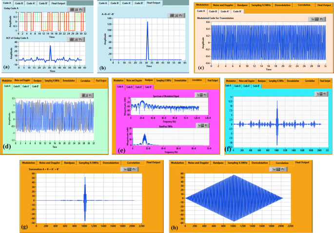
a Time series and ACF plots of 32 bit code A, b sum of the ACFs of codes A, B, A’, and B’, c modulated 206.5 MHz RF with code A, d modulated signal with noise, variance and Doppler added, e spectrum (in dB) of the modulated signal and the band-limited signal, f cross-correlated output of the signal modulated with code A. The sum of the cross correlated outputs of the four consecutive signals modulated, g using the codes A, B, A’ and B’, and h uncoded mode
-
(b)
Generates the modulated carrier wave at 206.5 MHz for 4, 8, 16, 32 bit code pairs in the order A, B, A’, and B’ (e.g. Fig. 6c).
-
(c)
Generates Gaussian noise with user-defined mean and variance added to the modulated signal. User defined Doppler is also added, to form a simulated received signal (e.g. Fig. 6d).
-
(d)
Plots the spectrum of the generated signal (e.g. Fig. 6e)
-
(e)
Produces the band-limit signal achieved using a bandpass filter of 5 MHz bandwidth (e.g. Fig. 6e).
-
(f)
Samples the filtered signal at a frequency of 9.5 MHz (undersampling) [18], and generates the In-phase (I) and Quadrature-phase (Q) signals of the resulting waveform.
-
(g)
Performs decoding of the filtered signals by performing cross-correlation with original transmit signal for the respective code sequences (e.g. Fig. 6f).
-
(h)
Generates the final output by summing the cross correlated outputs of the pulses during four radar sweeps. (e.g. Fig. 6g for coded mode, and Fig. 6h for uncoded mode of operation)

4 Discussion
Radar, an active remote sensing tool has gained immense popularity in atmospheric research. It is capable of making measurements from a range of heights simultaneously with high temporal and spatial resolution as compared to the in situ measurements, and under different atmospheric conditions. However, due to certain limitations or restrictions involved during transmission, it sometime pose a challenge in retrieving very weak back-scattered signals at fine resolution. One of the most popular and effective technique to overcome this signal detectability problem without compromising with the resolution, ΔR is pulse compression [26]. Past studies have shown that the demonstration and realization of this technique can be achieved through simulation or GUI based approach (e.g. [27, 28]). However, none of the reported studies discussed the application of this technique in detail. Therefore, the present work covers the demonstration and realization of this pulse compression technique in a 206.5 MHz atmospheric radar by including variety of attributes (e.g. PW, PRF, amplitude, noise, variance) and selection ranges (e.g. code selection from 4–32 bits, FFT points ranging from 256–4096).
The developed GUI tool shown in the preceding section performs the task of modulating the complementary code sequences onto the carrier frequency during transmission, while during reception, the tool is used to correlate and combine the signals using the same sequence of codes used in transmission. The type of modulation that has been used in the analysis and front-end GUI creation is phase modulation. Phase modulation occurs when the amplitude and frequency remain constant but the phase within the carrier frequency changes over a small range. The change in phase (polarity or direction of wave travel) is related directly to the digital information comprising the transmitted information. The pulse compression technique results in achieving ΔR of a short pulse at practically acceptable transmit peak power levels.
If \(A_{T} = \left\{ {a_{1} ,a_{2} ,a_{3} , \ldots a_{N} } \right\}\) and \(B_{T} = \left\{ {b_{1} ,b_{2} ,b_{3} , \ldots b_{N} } \right\}\), where, \(a_{i} ,b_{i} \in \left\{ { - 1, + 1} \right\}\) for \(1 \le i \le N\), then the coded transmitted radar signal is represented as:
where the width of each pulse (bit) in a code is called baud width (\(\tau\)), and the number of bits in the code is referred as baud length (N). The PW is computed as \(N \times \tau\). The angular frequency, \(\omega_{c} = 2\pi f_{c}\), IPP is the pulse repetition time (PRT), and \(rect\)() is the rectangular function.
The transmit RF signal in a given IPP is only available during the pulse width duration where its phase is altered according to the first code AT, and after some blanking period, the system waits for the returns until the start of the next cycle of IPP, where code BT is used for coding. In practical radar operation, generally four IPP cycles are used for reliable coded transmission, and the coding sequence follows \(A_{T}\), \(B_{T}\), \(A_{T}^{'}\) and \(B_{T}^{'}\), where, \(A_{T}^{'}\) and \(B_{T}^{'}\) are the complements of \(A_{T}\) and \(B_{T}\), respectively. The same sequence is repeated in the next four IPP cycles and so on, as long as the radar operation continues. On the other side, in atmospheric radar, the received signal Rx(t) is the time-shifted (delayed by time to) replica of the transmitted signal Tx(t) plus the additive noise n(t), given by:
In this equation, Tx(t) is expressed by Eq. (4). The noise and shifts in the Doppler frequency (fd = 1/to) may causes the ACFs of the complementary pairs to lose their ideal properties, resulting in the undesired side-lobes not being completely cancelled out, in practical radar application. These leftover side-lobes may suppress the detection from small targets or may cause false target detection. One possible approach to mitigate such problems to arise is proper selection of the complementary code pairs. The good complementary pair is the one that has very high merit factor and discrimination, and extremely low ISL and PSL [23].
5 Conclusion
The designed and developed front-end GUI has demonstrated the successful application to the pulse compression technique in the atmospheric radar at ~ 200 MHz, installed at one of the pristine sites (Nainital) located in the central Himalayan region. The atmospheric radar at 200 MHz frequency band itself is a novel choice which are quite limited in number (< 4) as compared to the similar radars available at ~ 50 MHz and ~ 400 MHz (> 30). User friendly GUI with its variety of attributes (e.g. PW, PRF, amplitude, noise, variance) and selection ranges (e.g. code selection from 4–32 bits, FFT points ranging from 256–4096) makes it plausible enough to be used and test the performance verifications of pulse compression technique in atmospheric radars operating in the VHF and UHF band, which are mainly employed for vertical wind profiling of the atmosphere. While the focus of this article is on atmospheric radar, however, the theory and approach presented may be useful to several other active remote sensing applications where pulse compression is needed.
References
Rouyer J, Mensah S, Vasseur C, Lasaygues P (2015) The benefits of compression methods in acoustic coherence tomography. Ultrason Imaging 37:205–223
Carpentier MH (1979) Evolution of pulse compression in the radar field. In: 9th European microwave conference, Brighton, UK. pp 45–53. https://doi.org/10.1109/EUMA.1979.332676
Ankarao V, Srivatsa S, Sundaram GAS (2017) Evaluation of pulse compression techniques for X-band radar systems. In: 2017 International conference on wireless communications, signal processing and networking (WiSPNET), Chennai, pp 1287–1292. https://doi.org/10.1109/WiSPNET.2017.8299971
O’Hora F, Bech J (2007) Improving weather radar observations using pulse-compression techniques. Meterol Appl 14:389–401. https://doi.org/10.1002/met.38
Le Chevalier F (2002) Principles of radar and sonar signal processing. Artech House, Boston, pp 1–416
Chelton DB, Walsh EJ, MacArthur JL (1989) Pulse compression and sea level tracking in satellite altimetry. J Atmos Ocean Technol 6:407–438. https://doi.org/10.1175/1520-0426(1989)006%3c0407:PCASLT%3e2.0.CO;2
Balsley BB, Gage KS (1980) The MST radar technique: potential for middle atmospheric studies. Pure Appl Geophys 118(1):452–493. https://doi.org/10.1007/BF01586464
Fukao S, Hamazu K, Doviak RJ (2014) Radar for meteorological and atmospheric observations. Springer Jpn. https://doi.org/10.1007/978-4-431-54334-3
Skolnik M (2008) Radar handbook, 3rd edn. McGraw-Hill, New York
Roguin A (2002) Christian Johann Doppler: the man behind the effect. Br J Radiol 75(895):615–619
Atlas D (1990) Radar in meteorology. Am Meteorol Soc. https://doi.org/10.1007/978-1-935704-15-7
Woodman RF, Guillen A (1974) Radar observations of winds and turbulence in the stratosphere and mesosphere. J Atmos Sci 31:493–505. https://doi.org/10.1175/1520-0469(1974)031%3c0493:ROOWAT%3e2.0.CO;2
Gage KS, Balsley BB (1978) Doppler radar probing of the clear atmosphere. Bull Am Meteorol Soc 59:1074–1094. https://doi.org/10.1175/1520-0477(1978)059%3c1074:DRPOTC%3e2.0.CO;2
Strauch RG, Merritt DA, Moran KP, Earnshaw KB, van de Kamp JD (1984) The Colorado wind-profiling network. J Atmos Ocean Technol 1:37–49
Farley DT (1985) On-line data processing techniques for MST radars. Radio Sci 20(6):1177–1184. https://doi.org/10.1029/RS020i006p01177
Hocking WK (2011) A review of mesosphere–stratosphere–troposphere (MST) radar developments and studies, circa 1997–2008. J Atmos Sol Terr Phys 73(9):848–882. https://doi.org/10.1016/j.jastp.2010.12.009
Weintroub S (1967) Pulse compression and radar. Nature 216:409–410. https://doi.org/10.1038/216409b0
Kumar A, Bhattacharjee S, Naja M, Kumar P (2011) Front-end digital signal processing scheme for 206.5 MHz atmospheric radar application. Int J Adv Technol (IJoAT) 2(1):71–81
Barker RH (1953) Group synchronizing of binary digital systems. Commun Theory 4:273–287
Strelkov GM, Konovalova AV (2010) A Barker signal transmitted over an ionospheric path. J Commun Technol Electron 55(7):721–732. https://doi.org/10.1134/S1064226910070016
Damtie B, Lehtinen M, Orispaa M, Vierinen J (2007) Optimal long binary phase code-mismatched filter pairs with applications to ionospheric radars. Bull Astron Soc India 35:619–623
Golay MJE (1961) Complementary series. IRE Trans Inf Theory 7(2):82–87. https://doi.org/10.1109/TIT.1961.1057620
Kumar A, Shrivastava A, Bhattacharjee S, Kumar P, Naja M (2012) Generation, analysis and evaluation of bi-phase complementary pairs. Int J Adv Technol (IJoAT) 3(4):209–214
Hussain A, Rais M, Malik MB (2008) Golay codes in ranging applications. In: 8th IASTED WOC-2008, Canada, pp 159–162
Parker MG, Paterson KG, Tellambura C (2002) Golay complementary sequences. In: Proakis JG (ed) Wiley encyclopedia of telecommunications. Wiley, New York
Blunt SD, Mokole EL (2016) Overview of radar waveform diversity. IEEE Aerosp Electron Syst Mag 31(11):2–42. https://doi.org/10.1109/MAES.2016.160071
Nagajyothi A, Rajeswari KR (2013) Graphical user interface based signal generator for radar/sonar pulse compression codes. Int J Comput Appl 82(16):15–19
Mar TT, Mon SSY (2014) Pulse compression method for radar signal processing. Int J Sci Eng Appl 3(2):31–35
Acknowledgements
We gratefully acknowledge the developers of MATLAB and LabVIEW tools, and thankful to the vendors providing free exceptional online technical supports, and self-learning materials on these tools. Authors are thankful to ARIES Nainital, and IIT(ISM) Dhanbad for providing necessary support and facilities to carry out this research work.
Author information
Authors and Affiliations
Corresponding author
Ethics declarations
Conflict of interest
No potential conflict of interest was reported by the authors.
Additional information
Publisher's Note
Springer Nature remains neutral with regard to jurisdictional claims in published maps and institutional affiliations.
Rights and permissions
About this article

Cite this article
Kumar, A., Singh, N. & Anshumali Simulation and interactive approach based demonstration of pulse compression technique in atmospheric radar. SN Appl. Sci. 1, 1678 (2019). https://doi.org/10.1007/s42452-019-1737-0
Received:
Accepted:
Published:
DOI: https://doi.org/10.1007/s42452-019-1737-0