
Abstract
The denoising and detection of transient disturbances are two important subjects for power quality monitoring and analysis. To effectively denoise and detect transient disturbances under noisy conditions, an improved iterative adaptive kernel regression method is proposed in this paper. The proposed method has advantages in that it does not need to estimate the noise variance or a filter threshold, and has both denoising and detection capabilities for transient disturbances. Simulation results demonstrate that the proposed method provides excellent denoising effects, which can not only suppress noise effectively but also preserve disturbance features of sudden change points well. Additionally, it provides good detection and location performance for single and combined transient disturbances, even under strong noise conditions. Finally, the effectiveness of the proposed method is further verified by using real disturbance data.
1 Introduction
With the wide application of various types of electronic devices and the increasing use of nonlinear, impact, and unbalanced loads in recent years, the power quality (PQ) of power grids is getting declining [1, 2]. PQ monitoring and analysis, including data compression, denoising, detection, feature extraction, and classification, have become important aspects of power distribution networks for avoiding damage to equipment and determining the causes of disturbances [3, 4]. PQ issues in the power systems can be divided into steady-state and transient problems [5]. Transient PQ disturbances (PQDs), including voltage sag, voltage swell, voltage interruption, oscillation transient, and impulsive transient [5], have strong impacts on both the grid and customers, with potentially serious consequences [6]. Therefore, significant researches on transient PQD analysis are expected to increase in the immediate future. This paper focuses on two aspects of transient PQD analysis: denoising and detection.
In practice, PQ signals are often corrupted by white noise introduced by monitoring devices and transmission channels [2, 7]. Noise not only affects the extraction of important features from PQ signals, but also degrades the effectiveness of detection and classification methods [7]. Therefore, effective denoising of PQ signals is necessary and often performed as an initial step in many PQ signal-processing techniques [8]. An excellent transient PQD denoising method should have a good smoothing effect and strong ability to protect disturbance features at sudden change points. Otherwise, PQ signal denoising would be meaningless. A number of papers based on different techniques for PQ signal denoising, such as the wavelet transform (WT), empirical mode decomposition (EMD), mathematical morphology (MM), S-transform (ST), and hyperbolic S-transform (HST), have been published in recent years [8,9,10,11,12,13,14,15]. Among these techniques, WT is the most popular method and many WT-based denoising techniques have been proposed for PQ signal denoising [9,10,11,12]. Although these WT-based denoising methods have achieved some promising results, their denoising effect highly depends on the choice of mother wavelet and decomposition levels. The discrete WT exhibits varying levels of spectra leakage in certain subbands. Additionally, signals at boundaries are easily distorted. The performance of MM is determined by the choice of a morphological transform and the structural elements. If the type of morphological transform or shape and size of structural elements are chosen unreasonably, the denoising results for PQ signals will be seriously affected. When the structural elements of the closed operation are wider than the impulsive transients, the impulsive transients are treated as noise and filtered out [13]. The ST [14] cannot effectively preserve the disturbance features of sudden change points, and requires huge computational resources. As an improvement to the ST technique, HST can preserve the features of sudden change points more effectively than ST [15]. However, the HST still has the disadvantage of huge computational demand. Reference [8] applied two EMD-based denoising techniques to acquire denoised PQ signals and satisfactory classification results under noisy conditions. Although the EMD-based denoising techniques are proved to have better denoising results than ST in [8], their disadvantages were also made clear. The EMD leads to endpoint contamination and mode mixing [16]. Recently, [17] proposed an adaptive denoising method that can provide good denoising effects, but it has high computational demand.
Most existing PQ signal denoising methods must either estimate the noise variance or set a corresponding filter threshold. However, the noise variance of real PQ signals is typically unknown and difficult to estimate accurately. The filter threshold, which is crucial for PQ signal denoising, is also difficult to set accurately and automatically. If a large filter threshold is set, oversmoothing will occur. Conversely, a small filter threshold will result in inefficient denoising. Therefore, the practicality of these existing denoising methods is greatly limited. Kernel regression (KR) is an effective tool not only for the interpolation of regularly and irregularly sampled images but also for the restoration and enhancement of noisy sampled images. Reference [18] proposed the iterative adaptive KR (IAKR) method, which not only can suppress noise effectively but also has a strong ability to preserve the details of images such as the edges. However, there are almost no applications of IAKR in one-dimensional (1D) transient PQD denoising. To effectively denoise transient PQDs under strong noise conditions, an improved IAKR (IIAKR) method is proposed in this paper. The proposed method, which does not need to estimate the noise variance or filter threshold, has superiority when compared with previous methods.
Several approaches have been proposed for the detection of PQDs in recent years, including the discrete Fourier transform (DFT), short-time Fourier transform (STFT), Gabor-Wigner transform (GWT), Hilbert-Huang transform (HHT), WT, ST, Kalman filter (KF), and strong trace filter (STF) [19,20,21,22,23,24,25,26]. However, the DFT is not suitable for the detection of transient PQDs [19, 20]. The STFT [21, 22] has the limitation of a fixed window, so it is also inadequate for the analysis of transient signals. WT overcomes the main drawback of STFT, but its capabilities are often significantly degraded under noisy conditions [7, 20]. The GWT [23] has disadvantages of cross-term interference and heavy computational loads. Additionally, it must satisfy a synchronized sampling constraint [6]. The HHT leads to endpoint contamination during empirical mode decomposition, and is easily influenced by noise superimposed on signals [6, 24]. The ST [25] has the ability to detect disturbances under noisy conditions, but its computational demands are too high. Additionally, the Gaussian window function of the ST is inflexible. The KF [26] is the most popular parameter estimation method, but it cannot indicate the exact locations of transient PQDs. Furthermore, the KF trace has a delay in response to transient PQDs [6]. The STF [6], which is an enhancement of the KF, is also a parameter estimation method.
The IIAKR method proposed in this paper also has the capability to detect transient PQDs. To evaluate the effectiveness of the proposed method, experiments are performed with different types of transient PQDs under different noisy conditions. The experimental results demonstrate the effectiveness of the proposed method.
2 Basic principle of classic KR in 1D
In [18], the 1D data measurement model is defined as:
where yi is the measured data; xi is the coordinate of the measured data; z(·) is the regression function; εi is the independent and identically distributed zero-mean noise value; P is the number of sampling points within the kernel.
While the specific form of z(xi) may remain unspecified, if we assume that it is locally smooth to some order N, then we can estimate the value of the function at any point x given the data based on a generic local expansion of the function about that point. Specifically, if x is near the sample at xi, then we have the N-term Taylor series:
where β0= z(x), β1= z′(x), …, βN= z(N)(x)/N!.
If we assume the Taylor series is a local representation of the regression function, then estimating β0 can yield a local estimate of the regression function based on the data. Specifically, βn (n =1, 2, …, N) will provide localized information regarding the nth derivative of the regression function. Since this method is based on local approximations, a logical step is to estimate βn (n =0, 1, …, N) from the data while giving nearby samples higher weights than samples at greater distances. A weighted least-squares formulation capturing this idea in matrix form is equivalent to solving the following optimization problem:
where
In (5), K(·) is a kernel function that penalizes distance away from the local position where the approximation is centered. The global smoothing parameter h controls the strength of this penalty (smoothness of kernel estimation). K is a symmetric function that attains a maximum value at zero, satisfying:
where C is a constant value. The choice of the specific form of the function K is open and could be exponential, Gaussian, or any other form complying with the above constraints. It is known that for classic regression, the choice of the kernel only has a small effect on estimation accuracy. Therefore, preference is given to differentiable kernels with low computational complexity, such as the Gaussian kernel.
Since our primary interest is to compute an estimate of the signal, the necessary computations are limited to those that estimate β0, regardless of the estimator order N. Therefore, the least-squares estimation can be simplified as:
where e1 is a column vector with the first element equal to one and the other elements equal to zero. It should be noted that there is a fundamental difference between the case of N = 0 and a high-order estimator (N > 0) when computing β0.
3 IIAKR method for disturbance denoising and detection
3.1 Improved adaptive kernel regression
The kernel function in the classic kernel regression method only depends on spatial sample locations, but the adaptive kernel function in the adaptive kernel regression method proposed in [18] depends on sample locations and density, as well as the radiometric values of image data. Therefore, the adaptive kernel regression method has a greater ability to preserve image details, such as edges.
Adaptive kernel regression is structured similarly to (3) and framed as an optimization problem as follows:
where y, A, and β in 2D image processing are defined in [18], and are the same as those in (3) for the 1D case. Wadapt is defined as:
where Kadapt(·) is an adaptive kernel function that penalizes the spatial distance between the point of interest x and its neighbors {xi}, as well as the radiometric distance between the corresponding pixels y and {yi}, and is defined as:
where μi is a local density parameter (typically set as 1); Ci is a symmetric covariance matrix based on differences in local gray values. Because local edge structures are related to gradient covariance, an estimate for this covariance matrix can be obtained as follows:
where \( z_{{x_{1} }} ( \cdot ) \) and \( z_{{x_{2} }} ( \cdot ) \) are the first derivatives along x1 and x2 directions, respectively; wi is a local analysis window around the position of interest x.
Because the covariance in Ci describes the correlation between different dimensions, rather than different samples, it is clear that this covariance is not suitable for describing 1D transient PQ data. Therefore, the adaptive kernel regression method cannot be directly applied to transient PQD denoising and the following improvements are required.
In 2D image processing, Ci is based on differences in local gray values, whereas in the 1D case, it should be based on differences in local sample values. Therefore, Ci is redefined as:
In (13), the estimated value of Ci is entirely determined by local sample values ranging from yi−H to yi+H. For transient PQDs, larger Ci values can be obtained at sudden change points, but smaller Ci values will be obtained at other points. The parameter H controls the radius of a local analysis window and its value should be larger than one, but smaller than 1/10 of the cycle length of the analyzed signal. A larger H value should be chosen under strong noise conditions while a smaller H value should be chosen under weak noise conditions.
The Ci values are normalized as:
where L is the total number of sampling points.
The adaptive kernel function in the 1D case is modified as:
In (15), when the global smoothing parameter h is set to a larger value, the denoised signal will be smoother, but the accuracy of the estimated amplitudes of the sudden change points will decrease. In contrast, if h is set to be smaller, the denoised signal will be rougher, but the amplitude estimates of the sudden change points will be more accurate. Because h is a global smoothing parameter, once the value of h is fixed, the smoothing effect on all samples is the same. Therefore, a scheme must be implemented to reduce the h value at sudden change points to preserve transient PQD features and increase the h value at other points to obtain a good smoothing effect for effective noise suppression.
Because the sampling time interval for the input signal is a fixed value, the local density parameter μi in (15) should be set to one for all samples, meaning μi is not a meaningful parameter. To effectively suppress noise and preserve transient PQD features at sudden change points, μi is redefined in this paper, as shown in (16). In (16), if Ci > CT, then a μi value in the range of 0.25–1 can reduce the h value to preserve transient PQD features at the ith point which corresponds to a sudden change point. Otherwise, we maintain normal smoothing with a μi value of one at other points.
where α is a parameter satisfying 0 < α < 10, which controls the attenuation rate of μi; CT is the determinant threshold.
If we assume that the number of cycles of the input PQDs is M, then Ci can be divided into 4M data segments that do not overlap and have a fixed length of 1/4 of a cycle. If a data segment is defined as Sr (r = 1, 2, …, 4M), then CT is expressed as:
where median(·) indicates obtaining an intermediate value that decreases with an increase in the signal-to-noise ratio (SNR). Therefore, the obtained CT value also decreases with an increase in SNR.
The flow chart representation of the improved adaptive kernel regression method is presented in Fig. 1. In this flow chart, the input noisy PQ signal is utilized to estimate the Ci values based on (13) and (14). The Ci values are then utilized to estimate the adaptive kernel function Kadapt(xi − x, yi − y) (i = 1, 2, …, L) based on (15)–(17). Finally, the optimization problem is established based on (9) and solved by utilizing (8) to obtain the reconstructed (denoised) PQ signal \( \hat{\beta }_{0} \).

Flow chart of improved adaptive kernel regression method
3.2 IIAKR method
The flow chart representation of the IAKR method for image processing is presented in [18]. Therefore, it is not described in this section. In this paper, the IIAKR method for transient PQD denoising and detection is proposed. The flow chart of the proposed method is presented in Fig. 2, where u is the iteration number.

Flow chart of IIAKR method for transient PQD denoising and detection
In Fig. 2, the initial input \( \hat{\beta }_{0}^{(0)} \)for the first iteration is the input transient PQD. In the next iteration, the input, which is the denoised (reconstructed) transient PQD generated by the previous iteration, is utilized to calculate a more reliable reconstructed transient PQD. This process continues for u iterations. The output \( \hat{\beta }_{0}^{(u)} \), which is considered to be the most reliable reconstructed transient PQD, is the final denoising result. The output \( C_{i}^{(u)} \) is then utilized to perform transient PQD detection.
Let \( C = C_{i}^{(u)} \). In this paper, the specific steps for transient PQD detection and location are defined as follows.
Step 1: Estimate the threshold λ adaptively.
The threshold λ is crucial for transient PQD detection. It is known to be poor practice to artificially set a fixed λ value or different λ values for voltages with different levels of noise. Therefore, a scheme for automatically estimating the appropriate threshold λ is defined as:
where S is a matrix that stores the maximum amplitude of each 1/4 cycle of C; δ is a constant variable in the range of 0–1. It has been found that a δ value of 0.3 is typically reasonable, and this value is utilized in all the test cases presented in Section 4.2.
Step 2: Quantify the signal C by utilizing (19) to obtain the signal C′. According to the sharp information in C′, the detection and time localization of transient disturbances can be realized.
Parameters descriptions:
-
1)
The choice of order N affects the bias and variance of estimates [18]. In general, smaller values of N result in smoother reconstructed estimates (large bias and small variance). Conversely, overfitting occurs in regression when utilizing larger N values, resulting in more complex computations, small bias, and large estimation variance (transient PQD features are better preserved). The value of N must be a positive integer and is typically set to 2. The users can choose an optimal order according to their specific application environment.
-
2)
The number of sampling points within the kernel P must be odd, greater than 3, and less than 1/10 of the cycle length of the input signal. For a transient PQD in a low-SNR environment, a larger P value results in a better denoising effect (smoother disturbances), but its value should not be overly large. On the other hand, a smaller P value results in better preservation of disturbance features in high-SNR environments.
-
3)
While increasing the number of iterations reduces the estimation variance and increases the bias [18], it also leads to decreased capacity for preserving transient PQD features at sudden change points. Therefore, approximately 1–6 iterations are typically utilized and the minimum mean-squared error (MSE) of the reconstructed estimate can be obtained. An example of this observation is shown in Fig. 3. Figure 3a shows a voltage swell with SNR of 30 dB. By utilizing the IIAKR method with N = 2, P = 21, H = 5, h = 0.3, α = 2, δ = 0.3, and different iteration numbers, the analysis results of Fig. 3a are shown in Fig. 3b and c. Figure 3b shows the MSE values of the reconstructed voltage swell in different iterations. Figure 3c shows the amplitude errors (AEs) between the original and reconstructed signal at the 900th point (corresponding to the end point of the swell) in different iterations. Detailed explanation of AE will be given in Section 4.1. It can be observed in Fig. 3b and c that the minimum MSE is obtained in the fifth iteration and that the AE of the 900th sample increases with an increase in the number of iterations. Therefore, it is illustrated that the appropriate range of u is 1–6. Since the appropriate iteration number is small, the computational complexity of the proposed algorithm is relatively low.
Fig. 3 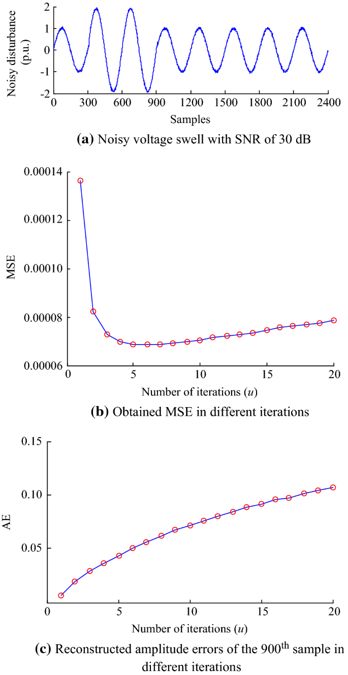
Results of applying IIAKR method with different iteration numbers

4 Results and discussion
To test the effectiveness of the IIAKR method for denoising and detecting transient disturbances, experiments are performed utilizing simulated and real transient data. Transient disturbances, including voltage sag, voltage swell, voltage interruption, impulsive transient, and oscillatory transient, are simulated utilizing MATLAB based on the mathematical models reported in [13] and [27]. All the simulated disturbances are created in eight cycles of a voltage waveform with a fundamental frequency of 50 Hz and sampling frequency fs of 15 kHz (300 sampling points each cycle and a sampling interval of Δt = 1/fs).
To simulate transient PQDs in noisy environments, ideal disturbance waveforms with diverse levels of white Gaussian noise are considered. The definition of SNR is given in (20) (unit: dB), where Ps and Pn refer to the average power of the ideal signal and the noise signals, respectively.
4.1 Denoising experiment for transient disturbances
SNR and MSE are typically utilized to evaluate the effectiveness of PQD denoising methods. However, these two indicators alone cannot accurately reflect the capability of methods to preserve disturbance features at sudden change points. Therefore, to better evaluate the effectiveness of the proposed method, the AEs between the original and reconstructed transient disturbances at the start and end points corresponding to the sudden change points are considered as an indicator in this study. The definition of AE is given in (21), where Ao and Ar refer to the original and reconstructed amplitude, respectively:
Oscillatory transient, voltage interruption, and voltage sag with SNR value of 25 dB are simulated and denoised by utilizing the IIAKR method. The denoised results are shown in Fig. 4a–c. The SNR values of the reconstructed signals in Fig. 4a–c rise to 35.0792 dB, 36.0230 dB, and 37.3386 dB, respectively, and the corresponding MSE values are 1.572 × 10⁻⁴, 9.37 × 10⁻⁵, and 7.5 × 10⁻⁵, respectively. For the oscillatory transient, the AE values at the start time (0.04073 s) and end time (0.06000 s) are 0.0812 p.u. and 0.0304 p.u., respectively. For the voltage interruption, the AE values at the start time (0.04007 s) and end time (0.08000 s) are 0.007922 p.u. and 0.02424 p.u., respectively. For the voltage sag, the AE values at the start time (0.02007 s) and end time (0.06 s) are 0.0101 p.u. and 0.0350 p.u., respectively. Figure 4 reveals that although the transient PQD signals are badly corrupted by noise, the reconstructed signals after applying the proposed method show good characteristics in terms of feature preservation and effective noise suppression.

Denoising results for disturbances with SNR of 25 dB utilizing IIAKR method
To further demonstrate the excellent denoising performance of the IIAKR method, its performance is compared with that of the wavelet method in [9]. Figure 5a shows a voltage swell with SNR of 30 dB and the denoised results after applying the proposed method and wavelet method in [9]. Figure 5b shows an impulsive transient with SNR of 30 dB and the corresponding denoised results after applying the two compared methods. As shown in Fig. 5a, the amplitudes of the denoised voltage swell at 0.008733 s and 0.06133 s (start and end time of the swell) are sharply reduced when utilizing the wavelet method, but are accurately preserved by the proposed method. As shown in Fig. 5b, the impulsive transient beginning at 0.03327 s and ending at 0.03333 s is largely filtered out by the wavelet method, but is accurately preserved by the proposed method. Figure 5 illustrates that the proposed method achieves better denoising performance than the wavelet method.

Denoising results after applying IIAKR method and wavelet method
By changing the SNR value of the noisy signals in Fig. 5, new noisy voltage swells and impulsive transients with SNR values ranging from 50 to 20 dB are created and analyzed by utilizing the proposed method (N = 2, P = 21, H = 5, h = 0.3, α = 2, δ = 0.3, u = 1 for SNR of more than 30 dB, and u = 3 for SNR of no more than 30 dB) and wavelet method (the mother wavelet is sym8, threshold rule is Heursure, decomposition level is 3, and tuning factors a and m are 0.3 and 3, respectively). SNR and MSE comparisons between the two methods are listed in Table 1. Comparisons of the AE at the start and end times of swells and pulses are listed in Tables 2 and 3. It should be noted that the results of the proposed method in Tables 1, 2 and 3 are not optimal and better results can be obtained if parameters are adjusted appropriately.
In Tables 1, 2 and 3, IIAKR represents the proposed method, while WT represents the wavelet method. In Tables 2 and 3, original represents the true amplitude of the ideal disturbance signal; AEIIAKR and AEWT represent the AE values of the IIAKR and WT method, respectively.
As shown in Table 1, the proposed method achieves approximately 3–14 dB better SNR values and smaller MSE values compared with the wavelet method. As shown in Tables 2 and 3, when the SNR is larger than 20 dB, the AE values of the reconstructed transient PQDs at the start and end times are approximately 0.0003–0.0596 p.u. when utilizing the proposed method, but 0.1309–0.2481 p.u. when utilizing the wavelet method. If the SNR is as low as 20 dB, the AE values increase when utilizing the proposed method, because the original transient PQD features are almost entirely buried by noise. However, the proposed method achieves much smaller AE values than the wavelet method, even if the SNR decreases to 20 dB. Tables 2 and 3 indicate that the proposed method has a stronger capability to preserve the characteristics of sudden change points for transient PQDs under different SNR conditions. Therefore, the results in Tables 1, 2 and 3 clearly demonstrate the effectiveness of the proposed method.
The adaptive denoising method [17] can effectively suppress noise and preserve transient PQD features at sudden change points. Therefore, the denoising performance of proposed method is also compared with that of the adaptive denoising method. Figure 6a presents an impulsive transient that begins at 0.03007 s and ends at 0.0304 s, where the SNR value is 20 dB. When utilizing the adaptive denoising method and proposed method, the denoised results for Fig. 6a are presented in Fig. 6b and c, respectively. The SNR values of the denoised signals in Fig. 6b and c rise to 30.4570 dB and 31.5819 dB, respectively, and the corresponding MSE values are 0.0018 and 3.489 × 10⁻⁴, respectively. Figure 6 demonstrates that the proposed method achieves slightly better denoising results compared with the adaptive denoising method. However, based on the results in Table 4, the computation time of the proposed method is only slightly longer than that of the wavelet method, but much shorter than that of the adaptive denoising method. Compared with the wavelet method and adaptive denoising method, the proposed method provides both good denoising results and short computation time and has significant advantages.

Denoising results after applying proposed method and adaptive denoising method
4.2 Detection experiment for transient disturbances
The proposed method not only has a good denoising effect, but also has good capability for transient PQD detection. To demonstrate the effectiveness of the proposed method for transient PQD detection, simulated single and combined transient disturbances are considered in this section.
-
1)
Single transient disturbance detection
By utilizing MATLAB, single transient PQDs, including the impulsive transient, voltage interruption, voltage sag, voltage swell, and oscillatory transient with SNR values ranging from 40 to 20 dB, are generated. These noisy transient PQDs are detected by utilizing the proposed method and the detection results for the transient PQDs with SNR of 20 dB are presented in Fig. 7, where the red dashed line is the estimated threshold λ. One can clearly see a spike in C in Fig. 7a and the two main spikes in C in Fig. 7b–d, which represent the occurrence of transient PQDs. However, there are many spikes in C in Fig. 7e. Oscillation identification can be performed when the number of spikes in each cycle is greater than one and time localization of the oscillations can be performed based on the first and last spikes. According to the estimated threshold λ and (19), the background noise can be easily filtered out, thereby reducing C to C′. The detection and time localization of transient PQDs can be realized by using the obtained C′. The true values, detected values, and errors of the start and end points of different transient PQDs with different SNR values, are listed in Table 5. As shown in Table 5, the time location errors of the proposed method are 0–2Δt, which reveals that the proposed method can accurately detect and locate the single transient PQDs in different SNR environments, even if the SNR value decreases to 20 dB.
Fig. 7 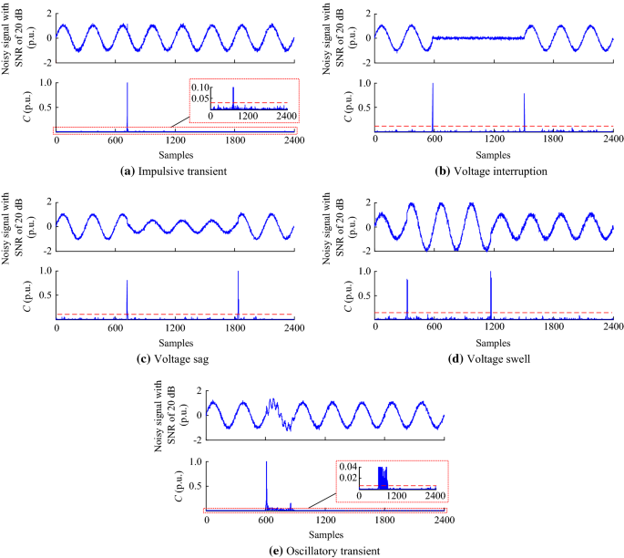
Detection results for transient disturbances with SNR of 20 dB
Table 5 Results for time localization of disturbances in Fig. 7 -
2)
Combined transient disturbance detection
Considering the space limitations for this paper, transient PQD detection experiments are performed utilizing only four types of combined transient PQDs with SNR of 25 dB, namely sag with swell (no overlap), sag with swell (overlap), interruption with oscillation (overlap), and interruption with oscillation (no overlap). The detection results when applying the proposed method are presented in Fig. 8, where the red dashed line is the estimated threshold λ. The results for time localization of the combined transient disturbances in Fig. 8 are listed in Table 6. The results in Fig. 8 and Table 6 demonstrate that the proposed method is effective for detecting and locating combined transient PQDs, even under strong noise conditions.
Fig. 8 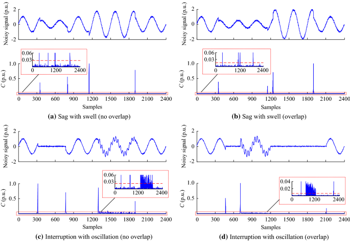
Detection results for the combined disturbances with SNR of 25 dB
Table 6 Results for time localization of combined disturbances in Fig. 8


4.3 Analysis of real data
The feasibility of the proposed method is also evaluated based on real transient disturbance data. Figure 9a presents a real transient disturbance with two small oscillations starting at approximately 0.02969 s and 0.07409 s, as well as a sag starting just after the first oscillation. When utilizing the wavelet method (the mother wavelet is sym8, threshold rule is Heursure, decomposition level is 3, and tuning factors a and m is 0.3 and 3, respectively), the denoising result for Fig. 9a is presented in Fig. 9b. When utilizing the proposed method with N = 2, u = 2, h = 0.3, P = 11, H = 7, α = 2, and δ = 0.3, the denoising and detection results for Fig. 9a are presented in Fig. 9c and d, respectively. Compared with Fig. 9b, c reveals that the proposed method provides a superior denoising effect, which not only makes the denoised signal smoother (as shown in the locally enlarged figures) but also accurately preserves transient disturbance characteristics. The red dashed line in Fig. 9d is the estimated threshold λ calculated based on (18). One can observe that the sharp information can be easily preserved according to the threshold. Figure 9d clearly identifies the occurrences of transient PQDs, which facilitates automatic signal processing by a computer.

Denoising and detection results for real disturbance data
5 Conclusion
The main purpose of this paper is to introduce a novel method to denoise and detect transient disturbances. The IAKR method is an effective image denoising tool that can not only suppress noise effectively, but also preserve the details in images, such as edges. Based on deep research of this method, the IIAKR method is proposed for transient PQD denoising and detection, which has the advantage of avoiding estimating noise variance and a filter threshold.
Experimental results demonstrate that the proposed method is effective in transient PQD denoising and can accurately preserve transient disturbance characteristics at sudden change points, even under strong noise conditions. Additionally, it yields good detection and location results for single and combined transient disturbances in different SNR environments. The proposed method has great potential for transient disturbance denoising and detection in PQ monitoring and analysis.
References
Singh U, Singh SN (2017) Application of fractional Fourier transform for classification of power quality disturbances. IET Sci Meas Technol 11(1):67–76
Li JM, Teng ZS, Tang Q et al (2016) Detection and classification of power quality disturbances using double resolution S-transform and DAG-SVMs. IEEE Trans Instrum Meas 65(10):2302–2312
Wang N, Li LC, Jia QQ et al (2011) Classification of power quality disturbance signals using atomic decomposition method. Proc CSEE 31(4):51–58
Manikandan MS, Samantaray SR, Kamwa I (2015) Detection and classification of power quality disturbances using sparse signal decomposition on hybrid dictionaries. IEEE Trans Instrum Meas 64(1):27–38
Liu ZG, Zhang QG (2014) An approach to recognize the transient disturbances with spectral kurtosis. IEEE Trans Instrum Meas 63(1):46–55
He SF, Li KC, Zhang M (2014) A new transient power quality disturbances detection using strong trace filter. IEEE Trans Instrum Meas 63(12):2863–2871
Dwivedi UD, Singh SN (2009) Denoising techniques with change-point approach for wavelet-based power-quality monito- ring. IEEE Trans Instrum Meas 24(3):1719–1727
Shukla S, Mishra S, Singh B (2014) Power quality event classification under noisy conditions using EMD-based de-noising techniques. IEEE Trans Ind Inf 10(2):1044–1054
Ke H, Gu J (2010) Wavelet threshold de-noising of power system signals. Proc CSU-EPSA 22(2):103–108
Li TY, Chen CL, Cheng WL et al (2007) Application of cross validation in power quality de-noising. Autom Electr Power Syst 31(16):75–78
Zhang M, Li KC, Hu YS (2010) A power quality signal de-noising algorithm based on wavelet domain neighbouring thresholding classification. Autom Electr Power Syst 34(10):84–89
Jia YT, Zhang DL, Zhang B (2013) Power quality disturbance data denoising and compression using signal’s scale-dependencies of wavelet coefficients. Autom Electr Power Syst 37(5):68–73
Zhao J, He ZY, Qian QQ (2009) Detection of power quality disturbances utilizing generalized morphological filter and difference-entropy. Proc CSEE 29(7):121–127
Yi JL, Peng JC, Luo A et al (2010) Power quality signals denoising using modified S-transform method. Chin J Sci Instrum 31(1):32–36
Jiao SB, Huang H, Zhang Q (2011) A new hyperbolic S-Transform based denoising method of power quality signals. Power Syst Technol 35(9):105–110
Qian Y, Huang CJ, Chen C (2005) Denoising of partial discharge based on empirical mode decomposition. Autom Electr Power Syst 29(12):53–56
Wang Y, Li QZ, Gao J (2016) Adaptive de-noising method for power quality disturbance signals. Autom Electr Power Syst 40(23):109–117
Takeda H, Farsiu S, Milanfar P (2007) Kernel regression for image processing and reconstruction. IEEE Trans Image Process 16(2):349–366
Lin CH, Wang CH (2006) Adaptive wavelet networks for power-quality detection and discrimination in a power system. IEEE Trans Power Deliv 21(3):1106–1113
Liao CC, Yang HT, Chang HH (2011) Denoising techniques with a spatial noise-suppression method for wavelet-based power quality monitoring. IEEE Trans Instrum Meas 60(6):1986–1996
Wright PS (1999) Short-time Fourier transforms and Wigner- Ville distributions applied to the calibration of power frequency harmonic analyzers. IEEE Trans Instrum Meas 48(2):475–478
Gu YH, Bollen MHJ (2000) Time-frequency and time-scale domain analysis of voltage disturbances. IEEE Trans Power Deliv 15(4):1279–1284
Cho SH, Jang G, Kwon SH (2010) Time-frequency analysis of power-quality disturbances via the Gabor-Wigner transform. IEEE Trans Power Deliv 25(1):494–499
Li P, Gao J, Xu D et al (2016) Hilbert-Huang transform with adaptive waveform matching extension and its application in power quality disturbance detection for microgrid. J Mod Power Syst Clean Energy 4(1):19–27
Dash PK, Panigrahi BK, Panda G (2003) Power quality analysis using S-transform. IEEE Trans Power Deliv 18(2):406–411
Abdelsalama AA, Eldesouky AA, Sallam AA (2012) Classification of power system disturbances using linear Kalman filter and fuzzy-expert system. Int J Electr Power Energy Syst 43(1):688–695
Lee CY, Shen YX (2011) Optimal feature selection for power- quality disturbances classification. IEEE Trans Power Deliv 26(4):2342–2351
Acknowledgements
This work is supported in part by the National Key R&D Program of China (No. 2016YFB1200401, No. 2017YFB1201103), and in part by the Program for Application of Cophase Power Supply Technology (No. 2018002).
Author information
Authors and Affiliations
Corresponding author
Additional information
CrossCheck date: 24 August 2018
Rights and permissions
Open Access This article is distributed under the terms of the Creative Commons Attribution 4.0 International License (http://creativecommons.org/licenses/by/4.0/), which permits unrestricted use, distribution, and reproduction in any medium, provided you give appropriate credit to the original author(s) and the source, provide a link to the Creative Commons license, and indicate if changes were made.
About this article

Cite this article
WANG, Y., LI, Q. & ZHOU, F. Transient power quality disturbance denoising and detection based on improved iterative adaptive kernel regression. J. Mod. Power Syst. Clean Energy 7, 644–657 (2019). https://doi.org/10.1007/s40565-018-0467-4
Received:
Accepted:
Published:
Issue Date:
DOI: https://doi.org/10.1007/s40565-018-0467-4