
Abstract
Geographic variations in reproductive traits are important for evolutionary biology, but often difficult to investigate because of the need for a large-scale survey and the ephemeral nature of secondary sexual characteristics. Here, using web image searches (Google Images and Twitter), we revealed large-scale geographic variations (>1500 km) in breeding timing and nuptial coloration in the mutually ornamented fish, Japanese dace (Tribolodon hakonensis). As this fish is easily caught and many anglers upload their photographs on the web, we were able to find a total of 401 high-resolution photographs from all over Japan. Breeding periods were determined from dates of photographs with/without nuptial coloration, which matched with previous studies. We also found that breeding periods might have advanced three weeks over the last 80 years in the Chitose River, potentially because of climate change. Additionally, the pattern of latitudinal cline for breeding timing revealed delayed timing in higher latitudes, although regional variations were also high. Finally, we quantified the patterns of nuptial coloration for this mutually ornamented fish, and confirmed that over 80% of individuals showed typical colorations, but others showed rare phenotypes that were never previously described, including an intermediate coloration between T. hakonensis and a potentially hybridizing species, T. brandtii. Our web-based method for estimating breeding phenology could be adopted for organisms with temporal sexual characteristics, such as plants (e.g., flowering time) and some fishes. Web image analyses are still preliminarily with many limitations, but could be promising for investigating variations in visible traits.
Introduction
Massive amounts of information have been made available on the web by people worldwide, and the quantity of information is growing at an overwhelming rate. Scientists are aware of the importance and usefulness of information on the web. In particular, biologists have tried to actively acquire data from citizens via web-based projects (e.g., eBird); that is, researchers encourage citizens to send biological information to the researchers’ websites or e-mail addresses. Such projects have successfully revealed phenology (Hurlbert and Liang 2012) and temporal changes in distribution (Taylor et al. 2014). However, in other research areas, such as linguistics and environmental science, researchers have been gathering information in an easier way by using internet search engines such as Google and Yahoo (e.g., Blair et al. 2002; Schade et al. 2013).
Three types of biological information can be obtained from web searches: search queries, videos, and photographs. These data often include dates and localities. Although the search query itself only represents citizen interest in the query, the frequency of searching for a certain organism could relate to the abundance of that organism, and temporal change in search frequency could represent temporal change in biological phenomena (i.e., phenology). In fact, search query frequency has been used to detect flu epidemics (e.g., Ginsberg et al. 2009), range expansion, and phenology via Google Trends (Proulx et al. 2014). Videos and photographs contain biological information, and could be used in various ways: videos can be used to study animal behavior (Nelson and Fijn 2013; Yamazaki and Koizumi 2017); photographs have been used to detect invasive species (Miyazaki et al. 2016), color variations between (Allen et al. 2013; Sanz et al. 2013) and within species (Leighton et al. 2016), and for morphological study. These topics are crucial for ecological and evolutionary studies, and ecosystem management, but are often difficult to study because long-term or wide-range surveys are required. Because web-based citizen science can be cost-effective and well suited to macro-ecology (Kobori et al. 2016), web search-based research is becoming increasingly popular (Newman et al. 2012; Proulx et al. 2014; Leighton et al. 2016).
Japanese dace (Tribolodon hakonensis), a cyprinid fish, is a potentially good target for citizen science. Because they are easy to catch by fishing, many anglers upload pictures on the web. Japanese dace is distributed in Far East Asia, and ranges from Kyushu to Sakhalin and Sea of Japan (Sakai 1995). In this fish, males and females exhibit remarkable nuptial coloration during breeding season (e.g., Nakamura 1969). Current theories argue that such mutual ornamentation evolves via mutual sexual selection (i.e., both males and females are sexually selected) and/or social selection (i.e., ornamentation reflects status regardless of sex) (reviewed in Kraaijeveld et al. 2007). However, the dace shows little territoriality (Ogawa and Katano 2016) and high promiscuity (Ito 1975); thus, the mutual nuptial coloration is enigmatic. This nuptial color is known to intra-specifically vary, and may be affected by hybridization with similar heterospecific, T. brandtii, in Russia (Sviridov et al. 2003). In Japan, geographic variation in coloration is suggested (Nakamura 1969), and hybridization with T. brandtii is also reported (Hokkaido, northeastern Japan; Sakai and Hamada 1985), but there has been no detailed description of nuptial color variation. Understanding inter- or intra-population variation in nuptial coloration could be important for revealing the function of this ornamentation. Additionally, because this species ranges widely in latitude, breeding period varies geographically: February to March in Kyushu, southwestern Japan (Tabeta and Tsukahara 1964), and July in Hokkaido, northeastern Japan (Okada 1935). However, reports of breeding periods are relatively sparse.
Here, we investigated the variations in breeding season and nuptial coloration in Japanese dace using web image searches with four specific analysis components. (1) First, we investigated the characteristics of photographs found from the web, such as locality and years, especially focusing on whether the frequency of photographs represent the relative abundance of the species (Ginsberg et al. 2009; Proulx et al. 2014). (2) Second, we estimated breeding periods based on the dates of photographs with/without nuptial coloration from three regions where breeding period has been reported. (3) Third, we evaluated latitudinal cline in breeding timing across Japan (ca. 1700 km), which is a basic but important macro-ecological pattern (e.g., O’Malley et al. 2010; Kobayashi and Shimizu 2013). (4) Finally, we assessed inter- and intra-population variations in nuptial coloration, and considered allopatric and sympatric distributions with the potentially hybridizing species T. brandtii. To our knowledge, this is the first study to estimate breeding season from web image searches, which might be a promising approach for phenology studies.
Methods
Web search methods
We slightly altered the search methods for photographs based on analysis components (Table 1). Web search was conducted over a total of eight days in November 2016 (8–10, 14, 17–18, 20, and 27; see Table 1).
-
1.
The first aim was to describe general characteristics of web photographs (e.g., frequency, locality, date). To find photographs from all over Japan with equal search effort among regions, we used the search query “Ugui” (the common name of Japanese dace in Japan), “Haya” (Japanese dace in the dialect of central and eastern Japan), or “Ida” (the dialect of western Japan) in Google Images. To find as many photographs as possible, we searched photographs every month from January 2008 to November 2016 by setting a custom date range (for example, we searched photographs uploaded from April to May 2008, then searched from May to June 2008). Exchangeable Image File Format (EXIF) data contain the date and time of photographs and camera settings, which are automatically recorded by the camera, and were used to investigate timing. If photographs did not contain EXIF data, photograph dates followed uploaders’ descriptions. Photograph localities followed uploaders’ descriptions, because none of the photographs contained localities in the EXIF data. Photographs without localities were omitted from the analyses. If uploaders did not describe the localities in detail, we defined their localities at the end point of the rivers described or the municipal office of the city, town, or village described. This should not significantly bias the results, because the potential maximum error (i.e., 0°35′27.60 in Sapporo city) is much smaller than the range we analyzed (i.e., 12°13′17.49 from Nobeoka, Kyushu to Teshio, Hokkaido). In addition, we only used only photographs with the date provided and visible nuptial coloration, because dace species in Japan can be easily distinguished by nuptial coloration. Species identification followed Amano and Sakai (2014) and the Japan Game Fish Association (2010); we omitted instances of nuptial coloration with broad black band and red cheeks (T. sachalinensis type) or one black and one red band (T. brandtii type, including two subspecies: T. b. maruta, which is distributed from Tokyo Bay to southern Iwate Prefecture; and T. b. brandtii, which is distributed from the Sea of Japan and Hokkaido; Sakai and Amano 2014) from analysis.
We also calculated the proportion of photographs that could be utilized for the analyses. We resampled photographs with nuptial-colored Japanese dace, and recorded the frequency of photographs for which the localities and dates were available. Here, we used “Ugui” as the search query and searched photographs every three month from 2014 to 2015. This search was conducted on 21 March 2017. Photographs found using this procedure were not used in the other analyses.
-
2.
To estimate local breeding periods, we compared the photograph dates with and without nuptial coloration (i.e., breeding and non-breeding status, respectively) within single rivers. We selected three rivers (Fig. 1a: Chikuma, Tama, and Chitose Rivers), because the estimated breeding periods were reported (Koyama and Nakamura 1955, Nakamura 1969 and Okada 1935, respectively) and enough photographs were available (>30 photographs) in these rivers. To find more photographs, we searched via Twitter in addition to Google Images. Because the three rivers are located in eastern Japan, the search queries were “Ugui” and “Haya,” which are the names of the dace in eastern Japan, combined with the name of the river (for example, “Ugui OR Haya Tama River”). Among the photographs without nuptial coloration, we selected the photographs that were clear enough to identify species from number of pre-dorsal scales or locality. In Tama and Chitose Rivers, because other similar species occur (T. brandtii and/or T. sachalinensis), we discarded the matching photographs that had more than 36 pre-dorsal scales (which is not in the range of Japanese dace, but of T. brandtii and T. sachalinensis) (Amano and Sakai 2014). As those two species are not distributed in Chikuma River, we did not select photographs based on scale number.
Fig. 1 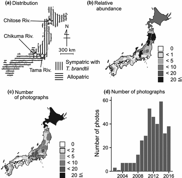
a Distribution of the Japanese dace, Tribolodon hakonensis, including sympatric and allopatric regions with a similar species with which it is potentially hybridizing, T. brandtii (T. b. maruta is distributed from Tokyo Bay to southern Iwate Prefecture, and T. b. brandtii is distributed from the Sea of Japan and Hokkaido: Sakai and Amano 2014). Stars indicate the three rivers where local breeding periods were estimated. b Relative abundances of Japanese dace calculated from the National Census on River Environments data. Numbers of photographs found for c each prefecture and d each year from 2002 to 2016
-
3.
To infer latitudinal cline, breeding timing was estimated from the dates of photographs with nuptial-colored Japanese dace. We used photographs from the above two procedures except for those without dates or nuptial coloration. In addition, to cover as many regions as possible, we searched specific regions where samples were sparse by adding the names of regions or rivers to the search query (e.g., “Ugui” OR “Haya” OR “Ida” “Osaka”).
-
4.
To elucidate variation in nuptial coloration, we selected the photographs based on the above three procedures. Photographs without dates were included in the analysis, and photographs with clear nuptial coloration were selected; photographs taken in turbid waters with nuptial-colored Japanese dace were omitted from the analysis.

Characteristics of photographs from the web
We summarized photographs from the web based on prefecture, and analyzed the relationship between number of photographs and relative abundance of Japanese dace. Here, we hypothesized that photograph frequency is correlated with local abundance or biomass of the species. However, it is difficult to estimate local abundance or biomass in many places. Therefore, we used the relative abundance (i.e., proportion of the target species to the total species) from a large nationwide dataset (described below). Relative abundance is widely used as a good surrogate for abundance or biomass (e.g., Wang et al. 1995; Pearce and Ferrier 2001). We also considered the effect of human population size, because the number of photographs uploaded to the web should also correlate with human population size.
We used three datasets: (1) the number of photographs in each prefecture, (2) relative abundance of Japanese dace in each prefecture calculated from National Census on River Environments data (data available at http://mizukoku.nilim.go.jp/ksnkankyo/03/index.htm; accessed 20 December 2016), and (3) human population size in each prefecture in 2014 (data available at Statistics Japan, http://www.stat.go.jp/data/nihon/02.htm; accessed 27 December 2016).
In the river census dataset, we chose the most recent dataset available for each river, and did not use datasets from before 2010. Datasets were available for at least one river in every prefecture, with a maximum of five datasets used for a single prefecture. The census was conducted throughout each year (four seasons per year), and, because we used data from all seasons, the dace should be detected if present even though Japanese dace partially migrate. In each river, the proportion of Japanese dace to all fishes captured were calculated from the catch per unit effort standardized by the National River Census. The relative abundance in each prefecture was estimated by averaging the dace proportions calculated from the rivers surveyed in the prefecture. We only used the individuals identified as Japanese dace (T. hakonensis), and did not use unidentified individuals (i.e., T. spp.) which can contain other species of Tribolodon.
We constructed a generalized linear model (GLM) with log link and Poisson error distribution. The number of photographs was used as a response variable, and the relative dace abundance and human population sizes were used as independent variables. All statistical analyses were performed using R (R Development Core Team 2016).
Local breeding period estimation
During breeding season, Japanese dace of both sexes show obvious nuptial coloration, which typically consists of a combination of three red/yellow and two black bands (Fig. 2b, c, Nakamura 1969). During non-breeding season, they show silver to greyish color with two inconspicuous grey bands (however, lowermost orange/red bands may occasionally exist; Nakamura 1969). Therefore, we assigned one of two scores to photographs: the dace showed obvious orange/red bands or patches, score 1; pale/no orange/red band or patches, score 0. When multiple individuals with different body colorations were in the same photographs, we separately scored those individuals. However, individuals showing the same coloration pattern within one photograph were treated as a single data point. Dates of photographs were transformed into the number of days from 1 January regardless of year (i.e., May 30 was transformed into 150); inter-year difference was not considered because of limited sample sizes.

a Schematic diagram of Japanese dace from seven regions used to evaluate nuptial coloration. b–h Some photograph examples of variations in nuptial coloration (b, c typical coloration with difference in the color of Rb1–2): b orange/red Rp1–2 and Rb1–2, and black/dark grey Bb1–2 sampled in Sapporo, Hokkaido; c orange/red Rp1–2, yellow Rb1–2, orange/red Rb3, and black/dark grey Rb1–2 in Chiba, central Honshu; d orange/red Rp1–2 and Rb1–2, and grey Bb1–2 sampled in Bibi River, Hokkaido; e grey Rp1, pale red Rp2, grey Rb1–2, pale red Rb3, and grey Bb1–2 sampled in Akkeshi, Hokkaido; f orange/red Rp1–2 and Rb1–3, and white/orange Bb1–2 in Gifu, central Honshu; g orange/red Rp1–2, Rb1–3, and Bb1–2 sampled in Fukuoka, Kyushu; and h orange/red Rp1–2 and Rb1, black/dark grey Rb2, orange/red Rb3, and black dark grey Bb1–2, which is an intermediate phenotype between Tribolodon hakonensis and T. brandtii maruta sampled in Tama River, Tokyo. i, j PCA results; samples from allopatric and sympatric areas with T. brandtii are shown as circles and triangles, respectively. i Sample sizes are represented by plot size, and color variations of each region are indicated by arrows. j Variations in allopatric/sympatric areas are represented as box plots, and variation ranges within rivers (Chikuma, Tama and Chitose) are shown. b–h were photographed by citizens or researchers, and printed with their permission. Color version is in the online article
As Japanese dace spawns from spring to early summer, the average scores of breeding color (presence = 1, absence = 0) should be lower from late summer to early spring, and higher in spring and early summer. Therefore, a quadratic relationship is expected between dates and color scores. Hence, we employed a logistic regression using the date and its quadratic term as explanatory variables. Here, the ranges of days for which regression lines predicted >0.5 color score were defined as estimated breeding periods. To reduce potential scoring biases, a single person (KA) scored all the photographs, and consistency was confirmed by a blind test that used 50 random photographs (94% of scores were consistent). We also confirmed little observer bias with an additional blind test: 96% of scores judged by another person were consistent.
Latitudinal cline in breeding timing
As spawning of Japanese dace is strongly affected by water temperature (e.g., Tabeta and Tsukahara 1964; Nakamura 1969), we expected a latitudinal cline in breeding timing, which is usually found in many taxa (e.g., O’Malley et al. 2010; Kobayashi and Shimizu 2013). Therefore, we regressed the dates of photographs that showed the individuals with nuptial coloration against latitude. We assumed that the regression line represented the mean breeding timing at the given latitude. Although estimating local breeding period requires a relatively large dataset (see “Local breeding period estimation” in the “Results”), collecting many photographs from nearby areas should allow insight into the mean breeding timing around the region. Altitude may also affect regional temperature (Caissie 2006), but we did not consider altitude, because altitude can be sensitive to error caused by uncertain photograph localities. Longitude was not considered either, because latitude and longitude were strongly correlated (r = 0.74).
Variation in nuptial coloration
Detailed coloration was evaluated based on seven features: Rp1 and Rp2, red patches on the head located on the upper operculum and lower cheek, respectively; Rb1, Rb2, and Rb3, red bands on the body located above Bb1, on the lateral line, and below Bb2, respectively; and Bb1 and Bb2, black bands on the body located between Rb1 and Rb2, and Rb2 and Rb3, respectively (Fig. 2a). We subjectively evaluated the colors with identifiable criteria: we did not use color hue from compressed photographs (e.g., jpeg and png), because actual color hue in those images at pixel scale may significantly differ from what we perceive (Stevens et al. 2007). Coloration of each region was categorized into four ranks (red/orange, 2; pale red/yellow, 1; silver/grey, −0; black/dark grey, −1). To reduce potential scoring biases, a single person (KA) scored all the photographs, and consistency was confirmed from a blind test that used 210 points from 30 random photographs (92.4% of scores were consistent). Additionally, 80.5% of scores were consistent with those from another person. When multiple individuals with different body coloration were taken in the same photograph, we separately scored those individuals. However, individuals that showed the same coloration in one photograph were treated as a single data point.
To reduce the dimensions of the data, principal component analysis (PCA) was conducted. By checking the contribution of each trait to PCs, we can easily evaluate overall trait combination patterns. As the first two PCs accounted for most of the variance (75.9%), we used PC1 and PC2 values in subsequent analyses.
Geographical pattern in nuptial coloration was investigated. First, we examined correlation between PC values and latitude, because secondary sexual traits often show a latitudinal cline that is more elaborate in lower latitudes (Chui and Doucet 2009; Kawajiri et al. 2009). Second, we assessed a potential effect of hybridization with T. brandtii on nuptial coloration (Sviridov et al. 2003) by comparing the variance and mean values of PCs between sympatric and allopatric areas using the F-test and Welch’s t test, respectively. Sympatric and allopatric areas were categorized at the basin scale based on Sakai and Amano (2014). Body conditions and environmental factors may affect nuptial coloration (e.g., Morrongiello et al. 2010). However, because such information was rarely described by uploaders, we could not consider those factors.
Results
Characteristics of photographs from the web
Overall, we found a total of 401 photographs of Japanese dace from most areas of Japan (Table 1); of the 42 prefectures in which Japanese dace were found during the National River Census and the 46 prefectures that make up their known range, we acquired Japanese dace photographs from a total of 39 prefectures. We were able to utilize approximately half of the photographs from the web: among the 115 resampled photographs with nuptial coloration, both locality and date were available for 43.5% of the photographs. Among 401 photographs, 136 photographs (33.9%) contained dates, but no photograph contained localities in their EXIF data.
The number of photographs found during this analysis component (characteristics of photographs from the web) varied among regions, from 0 (nine prefectures in western Japan) to 52 (Tokyo) (Fig. 1c). GLM showed that both dace relative abundance and human population size positively affected the number of photographs (P < 0.001, Fig. 1b; Table 2). Most photographs dated from 2002 to 2016 (Fig. 1d), with a rapid increase from 2008 to 2011. We also analyzed relative abundance and phenology with Google Trends: the overall pattern showed peaks during early summer–early autumn, which might represent spawning season, but regional analysis was impossible because of small sample sizes (Online Resource Fig. S1C).
Local breeding period estimation
We found 33, 98, and 72 photographs taken in Chikuma, Tama, and Chitose Rivers, respectively. Regression curves were convex-shaped in Tama and Chitose Rivers (Fig. 3b, c). In Tama River, estimated range was almost the same at the ending, and two weeks earlier at the beginning of the previously reported breeding period (Nakamura 1969). In Chitose River, length of the breeding period was four times longer, and the peak of the curve was approximately three weeks prior to the peak of the breeding period reported 80 years ago (Okada 1935). In Chikuma River, the regression curve was sigmoid-shaped, and its peak was located outside of the known breeding period, which is due to the lack of data from January to March. However, the ranges of the dates of photographed nuptial-colored fish were well within the reported breeding periods (Fig. 3a).

Estimation of breeding periods in a Chikuma, b Tama, and c Chitose Rivers by quadratic logistic regression. Photograph dates were calculated taking 1 January as day 1 (i.e., 30 May was transformed into 150). Dashed lines indicate the day for which the regression curve predicted 0.5 breeding color value. Solid lines indicate the breeding periods reported in previous studies (for the respective rivers, Koyama and Nakamura 1955; Nakamura 1969; Okada 1935)
Latitudinal cline in breeding timing
We found a clear latitudinal cline in the dates of photographs that showed individuals with nuptial coloration across the Japanese archipelago (Fig. 4), which revealed that the mean breeding period was delayed in higher latitudes. This relationship was still significant after removing samples from Tama, Chikuma, and Chitose Rivers (r = 0.27, P < 0.01), where sample sizes were large. Estimated breeding timing was within the reported breeding periods except for a few cases (Fig. 4). Estimated breeding timing is mid-March in Kyushu, which is the southern margin of the distribution, and May in northern Hokkaido, northeastern Japan. We also found large variations in the dates when the dace showed nuptial coloration within the same latitude, which can indicate regional variation or long breeding periods within the same rivers. Additionally, five individuals showed nuptial coloration in late August and early September.

Latitudinal cline in breeding timing of Japanese dace estimated from the dates of photographs with nuptial coloration. Photograph dates were calculated taking 1 January as day 1 (i.e., 30 May was transformed into 150). Vertical lines indicate previously reported breeding periods in a Matsuura River (northern Kyushu, Tabeta and Tsukahara 1964); b Toba (central Honshu, Ishizaki et al. 2009); c # Tama River (Tokyo, see Fig. 1a, Nakamura 1969); d Tochigi Prefecture (central Honshu, Iwamoto and Kanoki 1983); e # Chikuma River (central Chubu, see Fig. 1a, Koyama and Nakamura 1955); f Mu River (central Hokkaido, Sakai 1995); g # Chitose River (central Hokkaido, see Fig. 1a, Okada 1935); and h Teshio River (northern Hokkaido, Ito 1975). (Hash) Rivers for which breeding periods were also estimated in this study (Fig. 3). *P < 0.01, **P < 0.001
Breeding color analyses
Of the total of 313 photographs, 80.8% (253) showed the typical nuptial coloration reported in Nakamura (1969), with two red patches on the head (Rp1–2), three red (to yellow) bands (Rb1–3), and two black (to gray) bands (Bb1–2) (Fig. 2b–d). The other 60 individuals lacked some of the red patches/bands (i.e., showing silver/greyish color), but some general patterns (clusters) appeared. For example, 8.3% (26) lacked Rb1–2, 5.8% (18) lacked Rp1 and Rb1–2 (Fig. 2e), 3.5% (11) only lacked Rb2, and less than 1% lacked Rp2 and Rb3. Of the 11 individuals that lacked Rb2, three from Tama River had dark-grey Rb2 (Fig. 2h). Most individuals showed black to grey Bb1–2. However, in two individuals from central Honshu and northern Kyushu, Bb1–2 were orange/white and orange, respectively (Fig. 2f, g). Correlations in colorations of Rp2 to Rb3, Rb1 to Rb2, and Bb1 to Bb2 were strong (r > 0.80, P < 0.001 after Bonferroni correction), and those of Rp1–2 and Rb3 to Bb1–2 were significant but weak (−0.29 < r < − 0.22, P < 0.001 after Bonferroni correction, see Fig. 2i). This means that (1) red patches/bands largely co-vary positively, (2) two black bands co-vary positively, and (3) red patches/bands vary independently from black bands. We could not find orange/red spots within Bb1–2, which are frequently found in Primorye, Russia (Sviridov et al. 2003).
PC1–2 values were not significantly correlated with latitude (r = − 0.05, P = 0.44 and r = 0, P = 0.94 for PC1 and PC2, respectively). Additionally, variance and average of PC1 values did not differ between allopatric and sympatric regions with T. brandtii (average, t = − 0.46, P = 0.64, Welch’s t-test; variance, F = 1.30, P = 0.14, F-test). However, PC2 showed greater variance in allopatric regions (F = 0.44, P < 0.001, F-test), mainly because of the two individuals that had orange Bb1, as mentioned above (Fig. 2j), whereas average did not differ between allopatric and sympatric regions (t = − 1.70, P = 0.09, Welch’s t-test). Variations within Chikuma, Tama, and Chitose Rivers were large and overlapping but not equal (Fig. 2j).
Discussion
Potential of web-based data for studying reproductive biology
We demonstrated the usefulness of web-based citizen data to investigate breeding season and the associated latitudinal cline, and nuptial color variations of a mutually ornamented fish, Japanese dace. It is now widely recognized that global climate change significantly affects organismal phenology, including breeding period (Walther et al. 2002). Web image searching can facilitate comparison between current and past phenologies in a wide range of species. In our case, the mean breeding period of Japanese dace in Chitose River was mid-July in the 1930s (Okada 1935), but was estimated to be mid-June based on photographs taken after 2009, which might be due to climate change or anthropogenic impacts.
Breeding period can directly influence population divergence via temporal reproductive isolation (reviewed in Ketterson et al. 2015) and candidate genes for phenology, such as clock genes, are known to vary with latitude (e.g., O’Malley et al. 2010). Empirical evidence on the latitudinal cline of breeding phenology, however, is limited (but see Berthold 1996; O’Malley et al. 2010). We successfully estimated the latitudinal pattern of breeding timing in Japanese dace over 1500 km, with only several days of web searching. Differences of 30–40 days in average breeding timing might contribute to intra-specific divergence. Future research can utilize this geographic variation to elucidate the temporal and spatial components of genetic variations within this species.
We also found large variation in nuptial coloration across Japan. The variation had some common trends, such as correlated changes within similar color patches/bands (i.e., red–yellow or black–gray) but not between the color patches/bands. Variation within populations was also large, although some geographic patterns still existed. Nuptial color variation has been occasionally mentioned in Japanese dace (Nakamura 1969; Sviridov et al. 2003), but this web-based approach is the first to quantitatively describe the variation in Japan.
Web-based data collection is useful for species that are frequently photographed by citizens and their photograph localities are easy to obtain (e.g., not conserved species). In particular, we were able to use web photographs with a relatively high proportion (i.e., 43.5%) that had available locality and date data compared with another similar study (26% in Leighton et al. 2016). This is probably because many photographs were uploaded on anglers’ blogs, which provide accurate date and approximate localities (e.g., names of rivers, cities, or villages) in many cases. Phenological traits may be able to be estimated for species that (1) change body colorations or shapes (e.g., plants, cyprinid, and salmonid fishes) or (2) migrate to spawning habitat during breeding seasons (e.g., migratory birds). In addition, variations in coloration could be revealed using citizen photographs, especially in organisms with discrete traits such as number of bands/spots, which can prevent observational errors. Although coloration and morphology seem easy to analyze using citizen photographs, various potential biases may exist because these characteristics are highly sensitive for to photography conditions (e.g., light conditions such as weather, and distance and angle to the targets) (Stevens et al. 2007; Sanz et al. 2013). Therefore, as a first step, categorical analysis of multiple spots/bands/patches, as used in this study, is preferable.
Although a web-based approach is cost-effective for describing large-scale patterns, it is important to recognize some limitations. First, inter-annual variation was not considered in this study, because we could not find enough photographs within years. To estimate the breeding period, photographs from before, during, and after the breeding period were needed: we could not estimate the breeding period in Chikuma River, mainly because of the lack of photographs in the spring. A balanced, relatively large dataset is needed to evaluate inter-annual variations (possibly 50–100 photographs per year based on the three rivers examined). If breeding period varies among years, and if the dace with nuptial coloration are more likely to be photographed than non-nuptial-colored dace, our analyses could overestimate the length of the breeding period. Second, non-random sampling is suggested, because the number of photographs was affected by human populations and relative abundance of Japanese dace. In addition, if rivers are long and the fish spawn in several places with different timing within rivers, estimation will be more difficult, because detailed localities are barely available from web images (only the names of rivers or towns, villages, and cities were available for most photographs). Another potential sampling bias is that uncommon phenotypes might be more likely to be photographed. This could be problematic if researchers are trying to evaluate the frequency of morphs or variations. However, it may be beneficial for describing overall variation if citizens tend to take photographs of rare phenotypes. Third, we subjectively categorized colorations, because qualitative evaluation of color hue from compressed photographs (e.g., jpeg and png) can have some biases (Stevens et al. 2007). Nonetheless, Leighton et al. (2016) subjectively evaluated color patterns of various animals using citizen photograph data on the web, and yielded results consistent with previous studies. We believe that evaluated patterns in this study were biologically meaningful, because the consistency with a previous study was high: over 80% of individuals were categorized with the same coloration as reported by Nakamura (1969). In addition, repeatability between persons was fairly high: consistency with another person was (1) 96% for judging the presence or absence of nuptial color, and (2) 80.5% in categorizing color patterns. Higher repeatability in judging presence or absence than scoring coloration could be due to evaluation simplicity.
Some limitations will be rapidly overcome by methodological advances. In particular, by asking photographers to include a color reference and scale bars in high-resolution photographs (e.g., Casanovas et al. 2014), citizen-based science might allow us to quantitatively analyze color hue and investigate the effect of body size on coloration. Therefore, we started gathering photographs for scientific use on the web site “Ugui nuptial coloration project” (http://ugui-guigui.wix.com/ugui-guigui), in which we ask citizens to take pictures with some forms of scale information, such as tobacco cases and postcards. Finally, the reproductive behavior of Japanese dace can also be studied based on data from the web: over 40 videos on the spawning of Japanese dace and closely related species (T. brandtii and T. sachalinensis) were uploaded to YouTube as of 31 December 2016, which will facilitate comparative studies.
Potential factors that affect nuptial coloration
Although our nuptial coloration analyses were preliminary, several important findings were yielded: (1) color co-varied within black bands and red bands/patches but not between black and red bands/patches, (2) nearly 20% of individuals lacked a few red bands/patches with some exceptional phenotypes (see Fig. 2f–h), and (3) large color variations existed within rivers. We also found that variation in color pattern was greater in allopatric than sympatric areas with a closely related species, T. brandtii, which can potentially hybridize with T. hakonensis (Fig. 2j). Potential factors that affect nuptial coloration include the conditions of individuals, such as nutritional status (Craig and Foote 2001); local environment, such as predation risk (Andersson 1994) and light conditions (Reimchen 1989), and timing (Kodric-Brown 1998).
Nuptial coloration of Japanese dace varied at a small spatial scale (i.e., within rivers). Red/orange coloration in Japanese dace is based on carotenoids (Matsuno and Katsuyama 1976), which animals can only acquire from diet (Goodwin 1984). Carotenoids are plant-synthesized pigments; thus, their abundance and coloration should co-vary with primary productivity (Leavitt 1993). Japanese dace migrate to the ocean or reside in rivers (e.g., Sakai and Imai 2005), which can shape substantial variation in body size within rivers (Nakamura 1969). Therefore, such tactics might result in a nuptial color variation via nutritional status, as is known in salmonids (Craig and Foote 2001). In addition, because variations within spawning schools were small (we only found one or two phenotypes within each photograph), such variations may also be due to temporal change. For example, Nakamura (1969) stated that Rb3 occasionally existed in the non-breeding season, which indicates that each coloration component appears/disappears at different timing.
Together with variations within rivers, geographic variations in nuptial coloration may also exist, because unique phenotypes were found in some areas (Fig. 2f–h: central Honshu, northern Kyushu, and Tama River, respectively). Hybridization with T. brandtii might also change nuptial coloration, because the two species differ in the coloration: T. brandtii has one dark grey/black band on the lateral line and one red (not orange) band below the lateral line (Nakamura 1969; Sviridov et al. 2002; Sakai and Amano 2014). We found three samples with an intermediate phenotype in nuptial coloration: two obvious orange bands above and below the lateral line, and one dark grey band on the lateral line. These samples were photographed in Tama River (Fig. 2h), where both species are abundant. The number of pre-dorsal scales (33–35) was also intermediate between the two species: it was within the range of Japanese dace (29–36: Amano and Sakai 2014), but also the range of T. brandtii (34–41: the range of the subspecies T. b. maruta, Sakai and Amano 2014). Because cranial morphology of the three individuals resembled T. brandtii (cheek wider than eye diameter), these individuals may be T. brandtii. However, the presence of an orange band above the lateral line, which is a characteristic of Japanese dace, has never been reported in T. brandtii (Nakamura 1969; Sviridov et al. 2002; Sakai and Amano 2014). These individuals are potentially hybrids, although hybridization between the daces is rare in northeastern Honshu (Tohoku district: Hanzawa et al. 1984; Sakai et al. 2007). Further study utilizing genetic markers in unexplored regions, including Tama River, is required. If coloration in daces prevents heterospecific matings, as previously suggested (Gritsenko 1974), species-specific coloration should be more conserved in sympatric than allopatric areas, because there is no risk of hybridization in allopatric regions (i.e., reinforcement: e.g., Higgie and Blows 2008).
We also suggest that the nuptial coloration of Japanese dace may differ between Japan and Primorye, Russia: in Japan, red/orange spots were absent from black/grey bands and Rb2 rarely reached the caudal fin; alternatively, in Primorye, Sviridov et al. (2003) reported that spots tended to be present (approximately 40% of individuals surveyed) and Rb2 reached the caudal fin (approximately 90% of individuals). This could be due to either the conditional or environmental factors discussed above, or genetic differences; Japanese dace in the eastern Sea of Japan, including Primorye, are genetically different from those in the Japanese archipelago (Sakai et al. 2002; Polyakova et al. 2015).
Mutual ornamentation is taxonomically widespread, but its function is still debated (Kraaijeveld et al. 2007). Promising approaches include comparative studies that analyze inter- or intra-specific variations in mutual ornamentation or degree of sexual difference, and other ecological or social factors that affect natural/sexual/social selection. Our findings regarding nuptial color variation within/between populations provides a foundation for investigating ecological/social factors that affect mutual ornamentation. In addition, some uploaders in western Japan suggested that nuptial coloration is more elaborate in males than females. Citizen-based science could facilitate studies that focus on intra-specific variation in strength of sexual difference, which is important for revealing the function of mutual ornamentation.
Change history
29 March 2018
The article “Web image search revealed large-scale variations in breeding season and nuptial coloration in a mutually ornamented fish.
References
Allen WL, Baddeley R, Scott-Samuel NE, Cuthill IC (2013) The evolution and function of pattern diversity in snakes. Behav Ecol 24:1237–1250
Amano S, Sakai H (2014) Morphological differentiation and geographic distribution of two types of anadromous cyprinid Tribolodon brandtii. J Nat Fish Univ 63:17–32 (in Japanese with English abstract)
Andersson M (1994) Sexual selection. Princeton University Press, Princeton
Berthold P (1996) Control of bird migration. Springer-Verlag, Berlin
Blair I, Urland G, Ma J (2002) Using Internet search engines to estimate word frequency. Behav Res Methods Instrum Comput 34:286–290. doi:10.3758/BF03195456
Caissie D (2006) The thermal regime of rivers: a review. Freshw Biol 51:1389–1406. doi:10.1111/j.1365-2427.2006.01597.x
Casanovas P, Lynch H, Fagan W (2014) Using citizen science to estimate lichen diversity. Biol Conserv 171:1–8. doi:10.1016/j.biocon.2013.12.020
Chui CKS, Doucet SM (2009) A test of ecological and sexual selection hypotheses for geographical variation in coloration and morphology of golden-crowned kinglets (Regulus satrapa). J Biogeogr 36:1945–1957
Craig JK, Foote CJ (2001) Countergradient variation and secondary sexual color: phenotypic convergence promotes genetic divergence in carotenoid use between sympatric anadromous and nonanadromous morphs of sockeye salmon (Oncorhynchus nerka). Evolution 55:380–391. doi:10.1554/0014-3820(2001)055[0380:CVASSC]2.0.CO;2
Ginsberg J, Mohebbi MH, Patel RS, Brammer L, Smolinski MS, Brilliant L (2009) Detecting influenza epidemics using search engine query data. Nature 457:1012–1014. doi:10.1038/nature07634
Goodwin TW (1984) The biochemistry of the carotenoids. II, animals. Chapman and Hall, New York
Gritsenko OF (1974) Systematics of Far Eastern rudd of the genus Tribolodon (Leuciscus brandti) (Cyprindae). J Ichthyol 14:677–689
Hanzawa N, Taniguchi N, Shinzawa H (1984) Genetic markers of the artificial hybrids between Tribolodon hakonensis and T. sp. (Ukekuchi-ugui). Otsuchi Mar Res Cent Rep 10:11–17 (in Japanese)
Higgie M, Blows M (2008) The evolution of reproductive character displacement conflicts with how sexual selection operates within a species. Evolution 62:1192–1203. doi:10.1111/j.1558-5646.2008.00357.x
Hurlbert AH, Liang Z (2012) Spatiotemporal variation in avian migration phenology: citizen science reveals effects of climate change. PLoS One 7:e31662. doi:10.1371/journal.pone.0031662
Ishizaki D, Otake T, Sato T, Yodo T, Yoshioka M, Kashiwagi M (2009) Use of otolith microchemistry to estimate the migratory history of Japanese dace Tribolodon hakonensis in the Kamo River, Mie Prefecture. Nippon Suisan Gakkaishi 75:419–424. doi:10.2331/suisan.75.419
Ito Y (1975) Notes on the spawning habits of three species of genus Tribolodon in Hokkaido. Sci Rep Hokkaido Fish Hatch 30:39–42 (in Japanese)
Iwamoto K, Kanoki H (1983) Aquaculture of Japanese dace. Bull Tochigi Fish Exp Stn 8:1–16 (in Japanese)
Japan Game Fish Association (2010) https://www.jgfa.or.jp/news_o/detail.html?LM_NWS_ID=714. Accessed 14 Nov 2016 (in Japanese)
Kawajiri M, Kokita T, Yamahira K (2009) Heterochronic differences in fin development between latitudinal populations of the medaka Oryzias latipes (Actinopterygii: Adrianichthyidae). Biol J Linn Soc 97:571–580
Ketterson E, Fudickar A, Atwell J, Greives T (2015) Seasonal timing and population divergence: when to breed, when to migrate. Curr Opin Behav Sci 6:50–58. doi:10.1016/j.cobeha.2015.09.001
Kobayashi MJ, Shimizu KK (2013) Challenges in studies on flowering time: interfaces between phenological research and the molecular network of flowering genes. Ecol Res 28:161. doi:10.1007/s11284-011-0835-2
Kobori H, Dickinson J, Washitani I, Sakurai R (2016) Citizen science: a new approach to advance ecology, education, and conservation. Ecol Res 31:1–19. doi:10.1007/s11284-015-1314-y
Kodric-Brown A (1998) Sexual dichromatism and temporary color changes in the reproduction of fishes. Am Zool 38:70–81. doi:10.1093/icb/38.1.70
Koyama H, Nakamura K (1955) Census of cast-net fishing and analysis of the stock in Tribolodon hakonensis and Zacco platypus, Chikuma River, Nagano Prefecture. Bull Freshw Fish Res Lab 4:1–16 (in Japanese)
Kraaijeveld K, Kraaijeveld-Smit FJL, Komdeur J (2007) The evolution of mutual ornamentation. Anim Behav 74:657–677
Leavitt PR (1993) A review of factors that regulate carotenoid and chlorophyll deposition and fossil pigment abundance. J Paleolimnol 9:109–127
Leighton G, Hugo P, Roulin A (2016) Just Google it: assessing the use of Google Images to describe geographical variation in visible traits of organisms. Methods Ecol Evol 7:1060–1070. doi:10.1111/2041-210X.12562
Matsuno T, Katsuyama M (1976) Comparative biochemical studies of carotenoids in Fishes-XIII carotenoids in six species of Leuciscinaeous fishes. Bull Japan Soc Sci Fish 42:847–850 (in Japanese with English abstract)
Miyazaki Y, Teramura A, Senou H (2016) Biodiversity data mining from Argus-eyed citizens: the first illegal introduction record of Lepomis macrochirus macrochirus Rafinesque, 1819 in Japan based on Twitter information. ZooKeys 569:123–133
Morrongiello J, Bond N, Crook D, Wong B (2010) Nuptial coloration varies with ambient light environment in a freshwater fish. J Evol Biol 23:2718–2725. doi:10.1111/j.1420-9101.2010.02149.x
Nakamura M (1969) Cyprinid fishes of Japan: Studies on the life history of cyprinid fishes of Japan. Research Institute of Natural Resources, Tokyo (in Japanese)
Nelson XJ, Fijn N (2013) The use of visual media as a tool for investigating animal behaviour. Anim Behav 85:525–536
Newman G, Wiggins A, Crall A, Graham E, Newman S, Crowston K (2012) The future of citizen science: emerging technologies and shifting paradigms. Front Ecol Environ 10:298–304. doi:10.1890/110294
Ogawa H, Katano O (2016) Effects of pale chub Zacco platypus and Japanese dace Tribolodon hakonensis on the growth of each other. Nippon Suisan Gakkaishi 82:128–130 (in Japanese)
Okada S (1935) Spawning habits of “ugui”, Leuciscus hakonensis Günther. Zool Mag 47:767–783 (in Japanese)
O’Malley KG, Ford MJ, Hard JJ (2010) Clock polymorphism in Pacific salmon: evidence for variable selection along a latitudinal gradient. Proc R Soc Lond B Biol Sci 277:3703–3714
Pearce J, Ferrier S (2001) The practical value of modelling relative abundance of species for regional conservation planning: a case study. Biol Conserv 98:33–43
Polyakova N, Semina A, Brykov V (2015) Analysis of mtDNA and nuclear markers points to homoploid hybrid origin of the new species of Far Eastern redfins of the genus Tribolodon (Pisces, Cyprinidae). Russ J Genet 51:1075–1087. doi:10.1134/S1022795415110137
Proulx R, Massicotte P, Pépino M (2014) Googling Trends in conservation biology. Conserv Biol 28:44–51. doi:10.1111/cobi.12131
R Development Core Team (2016) R: a language and environment for statistical computing, ver 3.3.1. R Foundation for Statistical Computing, Vienna. http://www.R-project.org/. Accessed 3 Aug 2016
Reimchen TE (1989) Loss of nuptial color in threespine sticklebacks (Gasterosteus aculeatus). Evolution 43:450–460
Sakai H (1995) Life-histories and genetic divergence in three species of Tribolodon (Cyprinidae). Mem Fac Fish Hokkaido Univ 42:1–98
Sakai H, Amano S (2014) A new subspecies of anadromous Far Eastern dace, Tribolodon brandtii maruta subsp. nov. (Teleostei, Cyprinidae) from Japan. Bull Natl Mus Nat Sci Ser A 40:219–229
Sakai H, Hamada K (1985) Electrophoretic discrimination of Tribolodon species (Cyprinidae) and the occurence of their hybrids. Jpn J of Ichthyol 32:216–224
Sakai H, Imai C (2005) Otolith Sr:Ca ratios of the freshwater and anadromous cyprinid genus Tribolodon. Ichthyol Res 52:182–184. doi:10.1007/s10228-004-0264-0
Sakai H, Goto A, Jeon S-R (2002) Speciation and dispersal of Tribolodon species (Pisces, Cyprinidae) around the Sea of Japan. Zool Sci 31:1291–1303. doi:10.2108/zsj.19.1291
Sakai H, Saitoh T, Takeuchi M, Sugiyama H, Katsura K (2007) Cyprinid inter-generic hybridization between Tribolodon sachalinensis and Rhynchocypris lagowskii in Tohoku District. J Nat Fish Univ 55:45–52 (in Japanese)
Sanz E, Taubadel N, Roberts D (2013) Species differentiation of slipper orchids using color image analysis. Lankesteriana 12:165–173. doi:10.15517/lank.v0i0.11743
Schade S, Díaz L, Ostermann F, Spinsanti L, Luraschi G, Cox S, Nuñez M, Longueville B (2013) Citizen-based sensing of crisis events: sensor web enablement for volunteered geographic information. Appl Geomat 5:3–18. doi:10.1007/s12518-011-0056-y
Stevens M, Párraga CA, Cuthill IC, Partridge JC, Troscianko TS (2007) Using digital photography to study animal coloration. Biol J Linn Soc 90:211–237. doi:10.1111/j.1095-8312.2007.00725.x
Sviridov V, Ivankov V, Luk’yanov P (2002) Variation of breeding dress of eastern redfins of the genus Tribolodon: I. Tribolodon brandti and T. ezoe. J Ichthyol 42:485–490
Sviridov V, Ivankov V, Luk’yanov P (2003) Variability of breeding coloration in the genus Tribolodon: II. Tribolodon hakuensis. J Ichthyol 43:101–104
Tabeta O, Tsukahara H (1964) The spawning habits of the anadromous Ugui-minnow, Tribolodon hakonensis hakonensis (Günther), with reference to the fishery in the northern Kyushu. Sci Bull Fac Agric Kyushu Univ 21:215–225 (in Japanese)
Taylor SA, White TA, Hochachka WM, Ferretti V, Curry RL, Lovette I (2014) Climate-mediated movement of an avian hybrid zone. Curr Biol 24:671–676
Walther GR, Post E, Convey P, Menzel A, Parmesan C, Beebee TJC, Fromentin JM, Hoegh-Guldberg O, Bairlein F (2002) Ecological responses to recent climate change. Nature 416:389–395
Wang WX, Fisher NS, Luoma SN (1995) Assimilation of trace elements ingested by the mussel Mytilus edulis: effects of algal food abundance. Mar Ecol Prog Ser 129:165–176
Yamazaki C, Koizumi I (2017) High frequency of mating without egg release in highly promiscuous nonparasitic lamprey Lethenteron kessleri. J Ethol. doi:10.1007/s10164-017-0505-0
Acknowledgements
We appreciate D. Kishi, J. Nakajima, S. Nakamura, I. Sakagawa, and N. Suzuki for permitting publication of their pictures in this paper, and M. Shibata and I. Atsumi for participating in the blind test. We are grateful to anonymous reviewers and editors for constructive comments, C. Ayer for checking the English, and D. Nomi for statistical advice.
Author information
Authors and Affiliations
Corresponding author
Ethics declarations
Conflict of interest
The authors have no conflict of interest.
Additional information
The original version of this article was revised due to a retrospective Open Access.
Electronic supplementary material
Below is the link to the electronic supplementary material.
Rights and permissions
This article is published under an open access license. Please check the 'Copyright Information' section either on this page or in the PDF for details of this license and what re-use is permitted. If your intended use exceeds what is permitted by the license or if you are unable to locate the licence and re-use information, please contact the Rights and Permissions team.
About this article

Cite this article
Atsumi, K., Koizumi, I. Web image search revealed large-scale variations in breeding season and nuptial coloration in a mutually ornamented fish, Tribolodon hakonensis . Ecol Res 32, 567–578 (2017). https://doi.org/10.1007/s11284-017-1466-z
Received:
Accepted:
Published:
Issue Date:
DOI: https://doi.org/10.1007/s11284-017-1466-z