
Abstract
This paper analyses the regional variation of age-related depreciation rates for housing: firstly, using observations of single-family house prices, our analysis estimates housing market-specific age-cohort depreciation rates, while taking into account the heterogeneity in attributes, location, and state of maintenance. Secondly, we examine whether the derived depreciation rates correlate with determinants of the regional supply- and demand-side. Considering the durability of the housing stock and substitution effects in housing demand, we find that a rise in excess supply will not only lead to declining house prices in the aggregate, but also to a widening of relative house price differentials among houses at different ages.


Notes
Due to the prevailing incapability of measuring housing quality appropriately, building age usually serves as an approximation for all sources of depreciation instead. Thus, age-related housing depreciation does not distinguish between declining functionality, physical deterioration, and an increase in incidental cost for maintenance (e.g., Smith 2004; Francke and Minne 2017).
The age-related depreciation of housing is the key ingredient of the filtering theories in which old dwellings represent the housing supply for households with lower income.
This represents a consequence of an indispensably high building activity given the shortage of living space as well as of a tendency toward suburbanization caused by an increased degree of motorization.
This work is therefore related to a large strand of literature which estimates age-related depreciation rates on the basis of cross-sectional data and hedonic modelling. For a literature review see Malpezzi et al. (1987), Wilhelmsson (2008), and Francke and Minne (2017). For an empirical application of a repeat sales approach see Clapp and Giaccotto (1998) or Harding et al. (2007).
A higher proportion of land value decreases the absolute price differences of single properties and therewith the relative price differences in structural characteristics. Hence, assuming the proportion of structural building value to land value to differ, the regional variation in depreciation rates is also likely to be a phenomenon of the spatial diversity in the land-to-structural value ratio (e.g., Bostic et al. 2007; Bourassa et al. 2011; Bourassa, Hoesli, Scognamiglio, and Zhang 2011; Francke and Minne 2017).
The set of existing rules formulated in the DIN 4108 Waermeschutzbestimmung had no legal force.
Defined in the Waermeschutzverordnung WSchV’95.
The empirical strategy is related to the literature dealing with estimating the demand for housing attributes. See Bayer et al. (2016) for a current study and a literature review. Our primary issue under consideration is, however, to examine the regional variation in age-related depreciation rates. Therefore, the analysis does not go beyond the first stage of the Rosen (1974)-two-step approach.
See also Sect. 2. For comparison, we make use of a polynomial function of the second order, which is commonly used in housing literature, as well as unspecific decade depreciation rates, \(j\in[<1950\), 1950–60, 1970–80, 1990–00, 2000–10], which are not justified by changes in legal settlement.
There has been no consensus in the housing literature so far as to how one should control appropriately for locational effects. In the last two decades the traditional hedonic model has been augmented by methodologies from spatial statistics and econometrics (e.g., Basu and Thibodeau 1998; Dubin 1999). Bourassa et al. (2007) finds, however, that simple ordinary least squares models containing community dummies do well in terms of predictive ability.
We use a fixed number of neighbors, \(k=10\), for the spatial structure. For the time period, we use a fixed number of objects relying on the absolute dimension of offered objects. The general weighting matrix can be described as follows: \(W={\sum^{m_{s}}_{i=1}{\rho^{i}S_{i}}}/{\sum^{m_{s}}_{i=1}{\rho^{i}}}\), with \(S_{i}\) (\(i\in[1,m_{s}]\)) the spatial neighbor, \(m_{s}\) represents the predefined number of regarded neighbors; \(\rho\) (\(\in[0,1]\)) represents the decay parameter \(\rho\) (\(\in[0,1]\)) which measures the relative impact of the individual neighbors which is then set to \(0.7\) (results are however robust to changes in \(\rho\)). By using a lower triangular weighting scheme with a large temporal dimension, we avoid endogenous problems and can apply a simple least squares methods for estimation (Pace et al. 2000).
Clapp and Salavei (2010) show that their findings are robust when the ratio of interior size to mean interior size of new houses in proximity is used instead. Accordingly, the calculated intensity of a house j is given as follows: \(\textit{int}_{i}=\boldsymbol{X_{i,int}}/(\boldsymbol{X_{j,int}}\,\vline\,j\in\boldsymbol{S})/{n_{X}}\) whereby \(\boldsymbol{S}\) represents the vector of neighboring houses to object i, and \(\boldsymbol{X_{i}}\) contains \({n_{X}}=4\) variables: living space, living space to overall lot size, building age, elevated equipment, and modernized.
According to Clapp et al. (2012), there is a problem in the identification of significant positive option values with regard to measuring land value. Therefore, the positive option value has only been identified correctly if the marginal effect (the log price difference between a house with low intensity and the middle (omitted) category) for the lower quartiles is positive as well as if the difference between a low intensity and a high intensity is positive as well.
Though considering rental prices, Thomschke (2015) is the only German data-based housing study to consider quantile effects.
For a review of quantile regression methodology, with a detailed discussion of the truncation problem and estimation procedure by minimization of the weighted sums of absolute residuals, see e.g. Koenker and Hallock (2001).
Although the dependent variable represents estimates, we do not need to bootstrap standard errors, seeing as derived coefficients stem from separate estimations.
See Lerbs and Teske (2016) for a literature review on the house price-vacancy relation.
We use the ratio of land-to-structural value of new construction as this age-cohort represents the reference group for the relative depreciation scheme in the hedonic models. By use of structural and locational variables discussed in previous subsections, we control for intraregional differences in land value as well as structural characteristics, such as lot size and living space among age-cohorts.
Single-family houses are defined as detached and semi-detached houses. Special housing types, such as mansions, are not included. The analysis of relative price differences among various housing types may be part of future research.
Some regional districts (Emden, Hameln-Pyrmont, Luechow-Dannenberg, Wilhelmshaven) have been deleted from the overall sample due to a very low number of observations.
Potential buyers will have a stronger market position in housing markets with high excess supply, which in turn will increase the local bargaining bias (e.g., Harding et al. 2003).
This supports the hypothesis that excess supply will also lead to a selection and therewith to lower re-use probabilities of existing older houses, notably in housing market areas where the share of single-family houses is high.
Table 9 shows dynamics for selected regional variables from Lower Saxony together with dynamics for all German regions.
The labor market of Wolfsburg is strongly marked by the head offices of Volkswagen.
The highest and lowest vacancy rates for all residential houses can be found in Salzgitter (\(10.43\%\)) and Wolfsburg (\(1.39\%\)) respectively.
Form of presentation is strongly inspired by Clapp et al. (2012). Coefficients are declared as statistically significant if their p-value is smaller than 0.1. Empirical results are robust against smaller \(\alpha\) values. Estimation results with \(\alpha=5\) will be provided upon request. Huber-White robust standard errors are calculated.
Although empirical results reveal that the model with a polynomial function (that is commonly used in housing literature) and the model with specific age-cohorts depreciation scheme do not differ significantly in measure-of-fit, the latter is more appropriate for the analysis of regional differences in marginal effects.
Due to a low spatial density of micro data, we concentrate mainly on indirect neighborhood effects. For a more differentiated analysis of price effects of houses in direct proximity see Zahirovich-Herbert and Gibler (2014).
Our results are therefore in contrast to the findings of Clapp et al. (2012). This may stem from the fact that we already use a large set of variables to control for locational values. However, for an interpretation of significant option value in sub-markets, the results must be identified by the strategy proposed by the former.
Significance is assessed by bootstrapped standard errors and significance levels of \(\alpha=10\) or better. Pseudo R‑squared statistics are reported as well. Results are robust against smaller \(\alpha\) values. Empirical results for a critical value of \(\alpha=5\%\) as well as for the specification without spatial effects are not reported but will be provided upon request.
Fig. 4 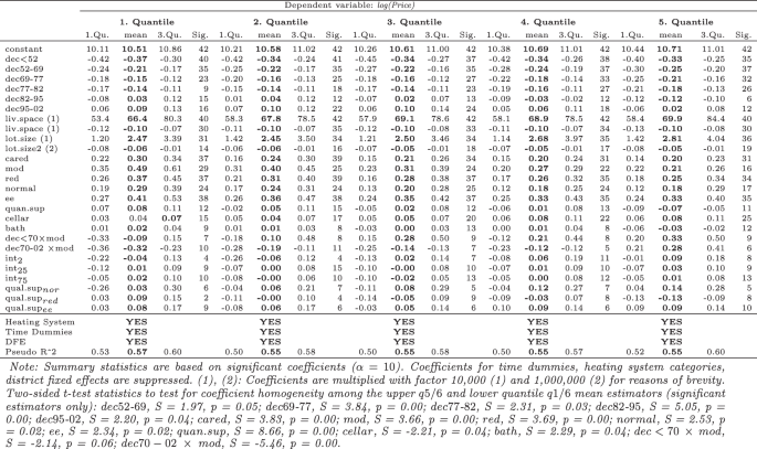
Quantile hedonic estimation results
For lack of describing the characteristics of the distribution-on-distribution of the estimators, we use t‑test statistics (two-sided) to test for coefficient homogeneity among the upper and lower quantile mean estimators in Fig. 4. Results are only reported for estimators that differ significantly.
Due to the relatively low number of observations, we present only selected estimation results with relevant accompanying variables. Empirical analyses on the basis of regional data often suffer from spatially correlated error terms due to omitted variables or spillover effects. To test for the presence of such phenomena, we use Moran’s I statistics, but do not find remaining autocorrelation in residuals.
There is however a strong correlation between vacancy rates and shares of age-cohorts on the total supply. We suggest that this stems from a long-term process: regions with steadily increasing population and low vacancy rates respectively are more likely to show a higher share of newly built houses. The endogeneity of new construction and deterioration is already discussed in the seminal paper of Sweeney (1974).
Offering prices, on the other hand, are likely to be biased due to bargaining effects. Hence, further research may deal with this problem in greater detail.

References
Arnott RJ, Braid RM (1997) A filtering model with steady-state housing. Reg Sci Urban Econ 27(4–5):515–546 (https://ideas.repec.org/a/eee/regeco/v27y1997i4-5p515-546.html)
Basu S, Thibodeau TG (1998) Analysis of spatial autocorrelation in house prices. J Real Estate Finance Econ 17(1):61–85 (https://ideas.repec.org/a/kap/jrefec/v17y1998i1p61-85.html)
Bayer P, McMillan R, Murphy A, Timmins C (2016) A dynamic model of demand for houses and neighborhoods. Econometrica 84:893–942 (https://ideas.repec.org/a/wly/emetrp/v84y2016ip893-942.html)
Bischoff O (2012) Explaining regional variation in equilibrium real estate prices and income. J Hous Econ 21(1):1–15 (https://ideas.repec.org/a/eee/jhouse/v21y2012i1p1-15.html)
Boehm TP, Ihlanfeldt KR (1986) The improvement expenditures of urban homeowners: an empirical analysis. Real Estate Econ 14(1):48–60 (https://ideas.repec.org/a/bla/reesec/v14y1986i1p48-60.html)
Bostic RW, Longhofer SD, Redfearn CL (2007) Land leverage: decomposing home price dynamics. Real Estate Econ 35(2):183–208 (https://ideas.repec.org/a/bla/reesec/v35y2007i2p183-208.html)
Bourassa S, Cantoni E, Hoesli M (2007) Spatial dependence, housing submarkets, and house price prediction. J Real Estate Finance Econ 35(2):143–160 (https://doi.org/10.1007/s11146-007-9036-8, https://ideas.repec.org/a/kap/jrefec/v35y2007i2p143-160.html)
Bourassa SC, Hoesli M, Scognamiglio D, Zhang S (2011) Land leverage and house prices. Reg Sci Urban Econ 41(2):134–144 (https://ideas.repec.org/a/eee/regeco/v41y2011i2p134-144.html)
Caplin A, Leahy J (2011) Trading frictions and house price dynamics. J Money Credit Bank 43:283–303 (https://ideas.repec.org/a/mcb/jmoncb/v43y2011ip283-303.html)
Chang Y, Chen J (2011) A consistent estimate of land price, structure price and depreciation factor. Technical Report, Freddie Mac Working Paper Series (Available at SSRN: https://ssrn.com/abstract=2296217 or http://dx.doi.org/10.2139/ssrn.2296217)
Clapp JM, Giaccotto C (1998) Residential hedonic models: a rational expectations approach to age effects. J Urban Econ 44(3):415–437 (https://ideas.repec.org/a/eee/juecon/v44y1998i3p415-437.html)
Clapp JM, Salavei K (2010) Hedonic pricing with redevelopment options: a new approach to estimating depreciation effects. J Urban Econ 67(3):362–377 (https://ideas.repec.org/a/eee/juecon/v67y2010i3p362-377.html)
Clapp JM, Bardos KS, Wong S (2012) Empirical estimation of the option premium for residential redevelopment. Reg Sci Urban Econ 42(1–2):240–256 (https://ideas.repec.org/a/eee/regeco/v42y2012i1p240-256.html)
Dubin RA (1988) Estimation of regression coefficients in the presence of spatially autocorrelated error terms. Rev Econ Stat 70(3):466–474 (https://ideas.repec.org/a/tpr/restat/v70y1988i3p466-74.html)
Dubin R, Kelley PR, Thibodeau TG (1999) Spatial autoregression techniques for real estate data. J Real Estate Lit 7(1):79–95
Francke MK, Minne AM (2017) Land, structure and depreciation. Real Estate Econ 45(2):415–451 (https://ideas.repec.org/a/bla/reesec/v45y2017i2p415-451.html)
Glaeser EL, Gyourko J (2005) Urban decline and durable housing. J Polit Econ 113(2):345–375 (https://ideas.repec.org/a/ucp/jpolec/v113y2005i2p345-375.html)
Gyourko J, Saiz A (2004) Reinvestment in the housing stock: the role of construction costs and the supply side. J Urban Econ 55(2):238–256 (https://ideas.repec.org/a/eee/juecon/v55y2004i2p238-256.html)
Harding JP, Knight JR, Sirmans C (2003) Estimating bargaining effects in hedonic models: evidence from the housing market. Real Estate Econ 31(4):601–622 (https://ideas.repec.org/a/bla/reesec/v31y2003i4p601-622.html)
Harding JP, Rosenthal SS, Sirmans C (2007) Depreciation of housing capital, maintenance, and house price inflation: estimates from a repeat sales model. J Urban Econ 61(2):193–217 (https://ideas.repec.org/a/eee/juecon/v61y2007i2p193-217.html)
Kholodilin KA, Menz JO, Siliverstovs B (2010) What drives housing prices down?: evidence from an international panel. J Econ Stat 230(1):59–76 (Jahrbuecher fuer Nationaloekonomie und Statistik)
Knight JR, Sirmans CF (1996) Depreciation, maintenance, and housing prices. J Hous Econ 5(4):369–389 (https://ideas.repec.org/a/eee/jhouse/v5y1996i4p369-389.html)
Koenker R, Hallock K (2001) Quantile regression: an introduction. J Econ Perspect 15(4):43–56
Lerbs O, Teske M (2016) The house price-vacancy curve. Tech. rep., ZEW Discussion Paper No. 16-082
Maennig W, Dust L (2008) Shrinking and growing metropolitan areas asymmetric real estate price reactions?: the case of German single-family houses. Reg Sci Urban Econ 38(1):63–69 (https://ideas.repec.org/a/eee/regeco/v38y2008i1p63-69.html)
Malpezzi S, Ozanne L, Thibodeau TG (1987) Microeconomic estimates of housing depreciation. Land Econ 63(4):372–385 (https://ideas.repec.org/a/uwp/landec/v63y1987i4p372-385.html)
Margolis SE (1981) Depreciation and maintenance of houses. Land Econ 57(1):91–105 (https://ideas.repec.org/a/uwp/landec/v57y1981i1p91-105.html)
McMillen DP (2008) Changes in the distribution of house prices over time: structural characteristics, neighborhood, or coefficients? J Urban Econ 64(3):573–589 (https://ideas.repec.org/a/eee/juecon/v64y2008i3p573-589.html)
Munneke HJ, Womack KS (2015) Neighborhood renewal: the decision to renovate or tear down. Reg Sci Urban Econ 54:99–115
Nappi-Choulet I, Maury TP (2011) A spatial and temporal Autoregressive local estimation for the Paris housing market. J Reg Sci 51(4):732–750 (https://ideas.repec.org/a/bla/jregsc/v51y2011i4p732-750.html)
Pace RK, Barry R, Gilley OW, Sirmans CF (2000) A method for spatial-temporal forecasting with an application to real estate prices. Int J Forecast 16(2):229–246 (https://ideas.repec.org/a/eee/intfor/v16y2000i2p229-246.html)
Rosen S (1974) Hedonic prices and implicit markets: product differentiation in pure competition. J Polit Econ 82(1):34–55 (https://ideas.repec.org/a/ucp/jpolec/v82y1974i1p34-55.html)
Rosenthal SS (2008) Old homes, externalities, and poor neighborhoods. A model of urban decline and renewal. J Urban Econ 63(3):816–840 (https://ideas.repec.org/a/eee/juecon/v63y2008i3p816-840.html)
Shilling JD, Sirmans C, Dombrow JF (1991) Measuring depreciation in single-family rental and owner-occupied housing. J Hous Econ 1:368–383
Smith BC (2004) Economic depreciation of residential real estate: microlevel space and time analysis. Real Estate Econ 32(1):161–180 (https://ideas.repec.org/a/bla/reesec/v32y2004i1p161-180.html)
Smith BA, Tesarek WP (1991) House prices and regional real estate cycles: market adjustments in houston. AREUEA J 19(3):396–416
Sweeney JL (1974) A commodity hierarchy model of the rental housing market. J Urban Econ 1(3):288–323 (https://ideas.repec.org/a/eee/juecon/v1y1974i3p288-323.html)
Thomschke L (2015) Changes in the distribution of rental prices in Berlin. Reg Sci Urban Econ 51(C):88–100 (https://ideas.repec.org/a/eee/regeco/v51y2015icp88-100.html)
Wilhelmsson M (2008) House price depreciation rates and level of maintenance. J Hous Econ 17(1):88–101 (https://ideas.repec.org/a/eee/jhouse/v17y2008i1p88-101.html)
Zahirovich-Herbert V, Gibler KM (2014) The effect of new residential construction on housing prices. J Hous Econ 26(C):1–18 (https://ideas.repec.org/a/eee/jhouse/v26y2014icp1-18.html)
Zietz J, Zietz E, Sirmans G (2008) Determinants of house prices: a quantile regression approach. J Real Estate Finance Econ 37(4):317–333 (https://ideas.repec.org/a/kap/jrefec/v37y2008i4p317-333.html)
Acknowledgements
The author thanks the editor and two anonymous reviewers for their very valuable comments.
Author information
Authors and Affiliations
Corresponding author
Appendix
Appendix
Rights and permissions
About this article

Cite this article
Gröbel, S. Regional heterogeneity in age-related housing depreciation rates. Rev Reg Res 38, 219–254 (2018). https://doi.org/10.1007/s10037-018-0125-3
Received:
Accepted:
Published:
Issue Date:
DOI: https://doi.org/10.1007/s10037-018-0125-3
Keywords
- Age-related housing depreciation
- Hedonic pricing model
- Regional housing markets
- Germany
- Single-family houses
Schlüsselwörter
- Altersbedingte Werminderung von Wohnimmobilien
- Hedonische Preisschätzung
- Regionale Wohnungsmärkte
- Deutschland
- Einfamilienhäuser