u–w formulation for dynamic problems in large deformation regime solved through an implicit meshfree scheme

Abstract

Solving dynamic problems for fluid saturated porous media at large deformation regime is an interesting but complex issue. An implicit time integration scheme is herein developed within the framework of the u–w (solid displacement–relative fluid displacement) formulation for the Biot’s equations. In particular, liquid water saturated porous media is considered and the linearization of the linear momentum equations taking into account all the inertia terms for both solid and fluid phases is for the first time presented. The spatial discretization is carried out through a meshfree method, in which the shape functions are based on the principle of local maximum entropy LME. The current methodology is firstly validated with the dynamic consolidation of a soil column and the plastic shear band formulation of a square domain loaded by a rigid footing. The feasibility of this new numerical approach for solving large deformation dynamic problems is finally demonstrated through the application to an embankment problem subjected to an earthquake.

A Appendix: Consistent linearization

As the linearization is referred to the undeformed domain, $B_0$, since it is time independent, it is necessary to move Eqs. (31–32) to the reference configuration. From the transport theorems we know that $dv=J \, dV$ and $ds=J\varvec{F}^{-T}dS$ and the Piola transformation states that $Div(\varvec{u})=J\, div(\varvec{u})$ (See [24, 35] for more information). Starting from these points, the equations to be linearized yield

$$\begin{aligned}&-\alpha _7\int _{B_0}\varvec{\tau }':\text{ grad }(\delta \varvec{u}) \, dV \; -\alpha _7\int _{B_0} Q \, \text{ Div }(\varvec{u}) \text{ div }(\delta \varvec{u}) \, dV\nonumber \\&\quad -\, \alpha _7 \int _{B_0} Q \, \text{ Div }(\varvec{w}) \text{ div }(\delta \varvec{u}) \, dV - \alpha _1 \int _{B_0} \left[ \rho _0\varvec{u}+J\rho _w \varvec{w}\right] \cdot \delta \varvec{u} \, dV \nonumber \\&\quad +\, \alpha _8 \int _{B_0} \rho _0\varvec{g}\cdot \delta \varvec{u} \, dV+ \alpha _8 \int _{\delta B_0} {\overline{\varvec{T}}}\cdot \delta \varvec{u} \, dS =0 \end{aligned}$$

(A.1)

$$\begin{aligned}&-\,\alpha _7 \int _{B_0} Q \, \text{ Div } (\varvec{u}) \text{ div }(\delta \varvec{w}) \, dV -\alpha _7 \int _{B_0} Q \, \text{ Div } (\varvec{w}) \text{ div }(\delta \varvec{w}) \, dV\nonumber \\&\quad - \,\alpha _4 \int _{B_0} \frac{J\mu _w}{k}\varvec{w} \cdot \delta \varvec{w} \, dV- \alpha _1 \int _{B_0} \frac{J\rho _w}{n}\varvec{w}\cdot \delta \varvec{w} \, dV\nonumber \\&\quad -\,\alpha _1 \int _{B_0} J \rho _w\varvec{u} \cdot \delta \varvec{w} \, dV + \alpha _8\int _{B_0} J \rho _w\varvec{g} \cdot \delta \varvec{w} \, dV\nonumber \\&\quad -\,\alpha _8\int _{\delta B_0}{\overline{\varvec{T}}}_w\cdot \delta \varvec{w} \, dS =0, \end{aligned}$$

(A.2)

where $\varvec{\tau }'$ is the effective Kirchhoff stress tensor and ${\overline{\varvec{T}}}$ and ${\overline{\varvec{T}}}_w$ are respectively the traction vectors of solid and fluid phases computed respect the undeformed configuration.

Before linearizing the different terms of the target equation, the linearization of some useful terms is carried out against $\varDelta \varvec{u}$:

$$\begin{aligned} D_u\left[ J\right] =J \, \text{ div }(\varDelta \varvec{u}) \end{aligned}$$

(A.3)

(From [16]) Also the linearization of n will be useful for the derivation of other quantities:

$$\begin{aligned} D_u\left[ n\right]= & {} D_u\left[ 1-\frac{1-n_0}{J}\right] =-(1-n_0)\frac{-1}{J^2}D_u\left[ J\right] \nonumber \\= & {} \frac{1-n_0}{J}\text{ div }(\varDelta \varvec{u})=(1-n) \text{ div }(\varDelta \varvec{u}) \end{aligned}$$

(A.4)

From tensor analysis [15] we determine that:

$$\begin{aligned} D_u\left[ \text{ grad }(\varvec{u})\right]= & {} D_u\left[ \text{ Grad }(\varvec{u}) \, \varvec{F}^{-1} \right] \nonumber \\= & {} \text{ Grad }(D_u\left[ \varvec{u} \right] ) \varvec{F}^{-1} + \text{ Grad }(\delta \varvec{u}) D_u\left[ \varvec{F}^{-1} \right] \nonumber \\= & {} \text{ Grad }(\varDelta \varvec{u}) \varvec{F}^{-1} - \text{ Grad }(\varvec{u}) \varvec{F}^{-1} \text{ grad }(\varDelta \varvec{u}) \nonumber \\= & {} \text{ grad }(\varDelta \varvec{u}) - \text{ grad }(\varvec{u}) \text{ grad }(\varDelta \varvec{u}) \end{aligned}$$

(A.5)

(A.6)

$$\begin{aligned} D_u\left[ \text{ Div }(\varvec{u})\right]= & {} D_u\left[ \varvec{I}: \text{ Grad }(\varvec{u})\right] =\varvec{I}:D_u \left[ \text{ Grad }(\varvec{u})\right] \nonumber \\= & {} \varvec{I}:\text{ Grad }(D_u\left[ \varvec{u}\right] )= \varvec{I}:\text{ Grad }(\varDelta \varvec{u})=\text{ Div } (\varDelta \varvec{u})\nonumber \\ \end{aligned}$$

(A.7)

So, the term we can see in the linear momentum balance equations is linearized as follows:

$$\begin{aligned} D_u\left[ \text{ Div }(\varvec{u})\text{ div }(\delta \varvec{u})\right]= & {} D_u\left[ \text{ Div }(\varvec{u})\right] \text{ div }(\delta \varvec{u})\nonumber \\&+\, \text{ Div }(\varvec{u})D_u\left[ \text{ div }(\delta \varvec{u})\right] \nonumber \\= & {} \text{ grad }(\delta \varvec{u}) : [ \text{ Div }(\varDelta \varvec{u})\varvec{I}\nonumber \\&-\, \text{ Div }(\varvec{u}) \text{ grad }^T(\varDelta \varvec{u})] \end{aligned}$$

(A.8)

Other important linearizations can be derived from Eq. A.4:

$$\begin{aligned} D_u\left[ k\right] =(1-n) \, \frac{\partial k}{\partial n}\, \text{ div }(\varDelta \varvec{u}) \end{aligned}$$

(A.9)

(See also [35])

$$\begin{aligned} D_u\left[ J\frac{\mu }{k}\right]= & {} \frac{\mu }{k}J \,\text{ div }(\varDelta \varvec{u})-J\frac{\mu }{k^2}D_u\left[ k\right] \nonumber \\= & {} J\frac{\mu }{k}\left[ 1-\frac{1-n}{k} \frac{\partial k}{\partial n} \right] \text{ div }(\varDelta \varvec{u}) \end{aligned}$$

(A.10)

$$\begin{aligned} D_u\left[ Q\right]= & {} D_u\left[ \frac{K_w}{n}\right] = K_w\frac{\partial }{\partial n}\left[ \frac{1}{n}\right] \, \frac{\partial n}{\partial \varvec{u}}=-\frac{K_w}{n^2}D_u[n]\nonumber \\= & {} -\frac{K_w}{n^2}(1-n) \text{ div }(\varDelta \varvec{u}) \end{aligned}$$

(A.11)

$$\begin{aligned} D_u\left[ J \frac{\rho _w}{n}\right]= & {} \frac{\rho _w}{n} J \, \text{ div }(\varDelta \varvec{u}) -J\frac{\rho _w}{n^2}(1-n) \text{ div }(\varDelta \varvec{u})\nonumber \\= & {} J \frac{\rho _w}{n}\frac{2n-1}{n}\text{ div }(\varDelta \varvec{u}) \end{aligned}$$

(A.12)

As the reference density is defined as

$$\begin{aligned} \rho _0= & {} J\rho =J \, n\rho _{w}+J(1-n)\rho _s\nonumber \\= & {} J \rho _{w}-(1-n_0)\rho _{w}+(1-n_0)\rho _s, \end{aligned}$$

(A.13)

the linearization of the density yields:

$$\begin{aligned} D_u\left[ \rho _0\right] =D_u\left[ J\rho _{w}\right] =J\rho _w \text{ div }(\varDelta \varvec{u}). \end{aligned}$$

(A.14)

The linearization will be stated for the weak form with respect to the reference configuration. Hereinafter the linearization of the terms that upon the deformation field are presented. All other terms will take part of the Newton scheme in the sense that it presented in Sect. 3. In the following equations superscripts represent the different terms of both Linear Momentum Balance equation of mixture and fluid phases respectively.

• $DG_{LMS} \cdot \varDelta \varvec{u}$:

  $$\begin{aligned} DG_{LMS}^{\; \;\;1} \cdot \varDelta \varvec{u}= & {} D_u\left[ \varvec{\tau }':\text{ grad }(\delta \varvec{u})\right] \nonumber \\= & {} \text{ grad }(\varDelta \varvec{u})\varvec{\tau }': \text{ grad }(\delta \varvec{u})\nonumber \\&+ \,J\,\text{ grad }(\varDelta \varvec{u}):\varvec{C}^{ep}: \text{ grad }(\delta \varvec{u})\nonumber \\ \end{aligned}$$

  (A.15)

  where $\varvec{C}^{ep}$ is the material elasto-plastic constitutive tangent operator. This linearization is widely developed in literature [40].

  $$\begin{aligned} DG_{LMS}^{\; \;\;2} \cdot \varDelta \varvec{u}= & {} D_u\left[ Q \, \text{ Div }(\varvec{u})\text{ div }(\delta \varvec{u}) \right] \nonumber \\= & {} D_u\left[ Q\right] \text{ Div }(\varvec{u})\text{ div } (\delta \varvec{u})\nonumber \\&+ \,Q \,D_u\left[ \text{ Div }(\varvec{u})\text{ div }(\delta \varvec{u})\right] \nonumber \\= & {} Q\,\left( -\frac{1-n}{n}\text{ div }(\varDelta \varvec{u}) \text{ Div }(\varvec{u})\text{ div }(\delta \varvec{u})\right. \nonumber \\&+\left. \text{ grad }(\delta \varvec{u}) : \left[ \text{ Div }(\varDelta \varvec{u})\varvec{I}- \text{ Div }(\varvec{u}) \text{ grad }^T(\varDelta \varvec{u})\right] \right) \nonumber \\= & {} J\,Q \,\text{ grad }\bigg (\delta \varvec{u}) :(\text{ div }(\varDelta \varvec{u})\varvec{I}\nonumber \\&-\, \text{ div }(\varvec{u}) \left[ \text{ grad }^T(\varDelta \varvec{u})+\frac{1-n}{n} \text{ div }(\varDelta \varvec{u})\varvec{I}\right] \bigg ) \nonumber \\\end{aligned}$$

  (A.16)
  $$\begin{aligned} DG_{LMS}^{\; \;\;3} \cdot \varDelta \varvec{u}= & {} D_u\left[ Q\, \text{ Div }(\varvec{w})\text{ div }(\delta \varvec{u}) \right] \nonumber \\= & {} D_u\left[ Q\,\right] \text{ Div }(\varvec{w})\text{ div }(\delta \varvec{u})\nonumber \\&+\, Q\, D_u\left[ \text{ Div }(\varvec{w})\right] \text{ div }(\delta \varvec{u})\nonumber \\&+\, Q \, \text{ Div }(\varvec{w})D_u\left[ \text{ div }(\delta \varvec{u})\right] \nonumber \\= & {} -J\,Q\,\text{ grad }(\delta \varvec{u}) :( \text{ div }(\varvec{w}) [ \text{ grad }^T(\varDelta \varvec{u}) \nonumber \\&+ \frac{1-n}{n}\text{ div }(\varDelta \varvec{u})\varvec{I} ] ) \end{aligned}$$

  (A.17)
  $$\begin{aligned} DG_{LMS}^{\; \;\;4} \cdot \varDelta \varvec{u}= & {} D_u\left[ \rho _0\varvec{u}+J\rho _w\varvec{w}\right] \cdot \delta \varvec{u}\\= & {} D_u\left[ J\rho _w\right] \left( \varvec{u}+\varvec{w}\right) \cdot \delta \varvec{u} + J\rho \, D_u[\varvec{u}]\cdot \delta \varvec{u}\nonumber \\= & {} J \left[ \rho \varDelta \varvec{u} + \rho _w \text{ div }(\varDelta \varvec{u})\left( \varvec{u}+ \varvec{w}\right) \right] \cdot \delta \varvec{u}\nonumber \end{aligned}$$

  (A.18)

• $DG_{LMS} \cdot \varDelta \varvec{w}$:

  $$\begin{aligned} DG_{LMS}^{\; \;\;2} \cdot \varDelta \varvec{w}= & {} D_w\left[ Q \, \text{ Div }(\varvec{u})\text{ div }(\delta \varvec{u}) \right] =0 \end{aligned}$$

  (A.19)
  $$\begin{aligned} DG_{LMS}^{\; \;\;3} \cdot \varDelta \varvec{w}= & {} D_w\left[ Q \, \text{ Div }(\varvec{w})\text{ div }(\delta \varvec{u}) \right] \nonumber \\= & {} J\,Q \, \text{ grad }(\delta \varvec{u}) : \text{ div }(\varDelta \varvec{w})\varvec{I} \end{aligned}$$

  (A.20)

• $DG_{LMW} \cdot \varDelta \varvec{u}$:

  $$\begin{aligned} DG_{LMW}^{\; \;\;1} \cdot \varDelta \varvec{u}= & {} D_u\left[ Q \,\text{ div }(\varvec{u})\text{ div }(\delta \varvec{w}) \right] \nonumber \\= & {} J\,Q \,\text{ grad }(\delta \varvec{w}) :\left( \text{ div }(\varDelta \varvec{u})\varvec{I}\right. \nonumber \\&- \left. \text{ div }(\varvec{u}) \left[ \text{ grad }^T(\varDelta \varvec{u})+\frac{1-n}{n} \text{ div }(\varDelta \varvec{u})\varvec{I}\right] \right) \end{aligned}$$

  (A.21)
  $$\begin{aligned} DG_{LMW}^{\; \;\;2} \cdot \varDelta \varvec{u}= & {} D_u\left[ Q\, \text{ div }(\varvec{w})\text{ div }\delta \varvec{w} \right] \nonumber \\= & {} -J\,Q\,\text{ grad }(\delta \varvec{w}) :( \text{ div }(\varvec{w}) [ \text{ grad }^T(\varDelta \varvec{u})\nonumber \\&+\,\frac{1-n}{n}\text{ div }(\varDelta \varvec{u})\varvec{I} ] ) \end{aligned}$$

  (A.22)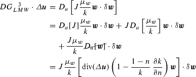
  

  (A.23)
  

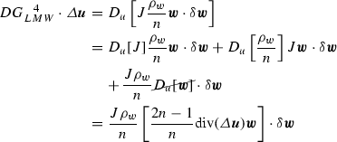  (A.24)
  $$\begin{aligned} DG_{LMW}^{\; \;\;5} \cdot \varDelta \varvec{u}= & {} D_u\left[ J\rho _w \varvec{u}\cdot \delta \varvec{w} \right] \nonumber \\= & {} \left[ D_u[J] \rho _w \varvec{u} + J\rho _w D_u[\varvec{u}]\right] \cdot \delta \varvec{w} \nonumber \\= & {} J \rho _w \left[ \varDelta \varvec{u}-\text{ div }(\varDelta \varvec{u})\varvec{u}\right] \cdot \delta \varvec{w} \end{aligned}$$

  (A.25)

• $DG_{LMW} \cdot \varDelta \varvec{w}$:

  $$\begin{aligned} DG_{LMW}^{\; \;\;1} \cdot \varDelta \varvec{w}= & {} D_w\left[ Q \text{ div }(\varvec{u})\text{ div }(\delta \varvec{w}) \right] =0 \end{aligned}$$

  (A.26)
  $$\begin{aligned} DG_{LMW}^{\; \;\;2} \cdot \varDelta \varvec{w}= & {} D_w\left[ Q \text{ div }(\varvec{w})\text{ div }(\delta \varvec{w}) \right] \nonumber \\= & {} J\,Q \, \text{ grad }(\delta \varvec{w}) : \text{ div }(\varDelta \varvec{w})\varvec{I} \end{aligned}$$

  (A.27)

Finally, using the different terms carried out in the Eqs. (A.15–A.27), the linearization of Eqs. (A.1–A.2) gives the following result:

$$\begin{aligned}&-\,\alpha _7 \int _B \text{ grad }(\delta \varvec{u}):\varvec{c}^{ep}: \text{ grad }(\varDelta \varvec{u}) \, dv\nonumber \\&-\,\alpha _7 \int _B \varvec{\sigma }':\text{ grad }^T (\delta \varvec{u} )\, \text{ grad }(\varDelta \varvec{u}) \, dv\nonumber \\&-\,\alpha _7 \int _B\text{ grad }(\, \delta \varvec{u}) :\left( Q\left[ \text{ div }(\varDelta \varvec{u})+\text{ div } (\varDelta \varvec{w}) \right] \varvec{I}\right) dv\nonumber \\&-\,\alpha _7 \int _B\text{ grad }(\, \delta \varvec{u}) : \left( p_w \left[ \text{ grad }^T(\varDelta \varvec{u})+\frac{1-n}{n}\text{ div } (\varDelta \varvec{u})\varvec{I} \right] \right) dv\nonumber \\&-\, \alpha _1\int _B \delta \varvec{u} \cdot \left[ \rho \varDelta \varvec{u} + \rho _w \varDelta \varvec{w} + \rho _w \text{ div }(\varDelta \varvec{u}) \left( \varvec{u}+\varvec{w}\right) \right] dv\nonumber \\&+ \,\alpha _8\int _B \rho _w \delta \varvec{u} \cdot \varvec{g} \, \text{ div }(\varDelta \varvec{u})\, dv \end{aligned}$$

(A.28)

$$\begin{aligned}&-\,\alpha _7 \int _B \text{ grad }(\, \delta \varvec{w}) :\left( Q\left[ \text{ div }(\varDelta \varvec{u})+ \text{ div }(\varDelta \varvec{w}) \right] \varvec{I}\right) dv\nonumber \\&-\,\alpha _7 \int _B \text{ grad }(\, \delta \varvec{w}) :\left( p_w \left[ \text{ grad }^T(\varDelta \varvec{u}) +\frac{1-n}{n}\text{ div }(\varDelta \varvec{u})\varvec{I} \right] \right) dv\nonumber \\&-\, \alpha _4 \int _B \frac{\mu _w}{k} \delta \varvec{w} \cdot \left[ \varDelta \varvec{w} + \text{ div }(\varDelta \varvec{u})\left( 1-\frac{1-n}{k} \, \frac{\partial k}{\partial n}\right) \varvec{w}\right] \, dv\nonumber \\&- \,\alpha _1\int _B\frac{\rho _w}{n} \delta \varvec{w} \cdot \left[ \varDelta \varvec{w} + \frac{2n-1}{n}\text{ div }(\varDelta \varvec{u})\varvec{w}\right] \, dv\nonumber \\&- \,\alpha _1 \int _B \rho _w \delta \varvec{w} \cdot \left[ \varDelta \varvec{u} + \text{ div }(\varDelta \varvec{u}) \varvec{u}\right] \, dv\nonumber \\&+\, \alpha _8\int _B \rho _w \delta \varvec{w} \cdot \varvec{g} \, \text{ div }(\varDelta \varvec{u})\, dv \end{aligned}$$

(A.29)

References

Arias-Trujillo J, Blázquez R, López-Querol S (2012) A methodology based on a transfer function criterion to evaluate time integration algorithms. Soil Dyn Earthq Eng 37:1–23
Armero F (1999) Formulation and finite element implementation of a multiplicative model of coupled poro-plasticity at finite strains under fully saturated conditions. Comput Methods Appl Mech Eng 171:205–241
Arroyo M, Ortiz M (2006) Local maximum-entropy approximation schemes: a seamless bridge between finite elements and meshfree methods. Int J Numer Meth Eng 65(13):2167–2202
Bandara S, Soga K (2015) Coupling of soil deformation and pore fluid flow using material point method. Comput Geotech 63:199–214
Biot MA (1956) Theory of propagation of elastic waves in a fluid-saturated porous solid. I. Low-frequency range. J Acoust Soc Am 28(2):168–178
Borja R, Alarcón E (1995) A mathematical framework for finite strain elastoplastic consolidation. Part1: balance laws, variational formulation, and linearization. Comput Methods Appl Mech Eng 122:145–171
Borja R, Tamagnini C, Alarcón E (1998) Elastoplastic consolidation at finite strain. pPart 2: finite element implementation and numerical examples. Comput Methods Appl Mech Eng 159:103–122
Cao T, Sanavia L, Schrefler B (2016) A thermo-hydro-mechanical model for multiphase geomaterials in dynamics with application to strain localization simulation. Int J Numer Methods Eng 107:312–337
Ceccato F, Simonini P (2016) Numerical study of partially drained penetration and pore pressure dissipation in piezocone test. Acta Geotech 12:195–209
Cividini A, Gioda G (2013) On the dynamic analysis of two-phase soils. In: Pietruszczak S, Pande GN (eds.) Proceedings of the third international symposium on computational geomechanics (ComGeo III), pp 452–461
Cuitiño A, Ortiz M (1992) A material-independent method for extending stress update algotithms from small-strain plasticity to finite plasticity with multiplicative kinematics. Eng Comput 9:437–451
Diebels S, Ehlers W (1996) Dynamic analysis of fully saturated porous medium accounting for geometrical and material non-linearities. Int J Numer Methods Eng 39:81–97
Ehlers W, Eipper G (1999) Finite elastic deformations in liquid-saturated and empty porous solids. Transp Porous Media 34:179–191
Gawin D, Sanavia L, Schrefler B (1998) Cavitation modelling in saturated geomaterials with application to dynamic strain localisation. Int J Numer Methods Fluids 27:109–125
Hughes T, Hilber H (1978) Collocation, dissipation and overshoot for time integration schemes in structural dynamics. Earthq Eng Struct Dyn 6:99–117
Hughes TJR, Pister KS (1978) Consistent linearization in mechanics of solids and structures. Comput Struct 8:391–391
Jeremić B, Cheng Z, Taiebat M, Dafalias Y (2008) Numerical simulation of fully saturated porous materials. Int J Numer Anal Methods Geomech 32:1635–1660
Lee E (1969) Elastic–plastic deformation at finite strains. J Appl Mech 36:1–6
Lewis R, Schrefler B (1998) The finite element method in the static and dynamic deformation and consolidation of porous media. Wiley, New York
Li B, Habbal F, Ortiz M (2010) Optimal transportation meshfree approximation schemes for fluid and plastic flows. Int J Numer Methods Eng 83:1541–1579
Li C, Borja RI, Regueiro RA (2004) Dynamics or porous media at finite strain. Comput Methods Appl Mech Eng 193:3837–3870
López-Querol S, Blazquez R (2006) Liquefaction and cyclic mobility model in saturated granular media. Int J Numer Anal Methods Geomech 30:413–439
López-Querol S, Fernández-Merodo J, Mira P, Pastor M (2008) Numerical modelling of dynamic consolidation on granular soils. Int J Numer Anal Methods Geomech 32:1431–1457
Marsden J, Hughes TJR (1983) Mathematical foundations of elasticity. Prentice Hall Inc., Upper Saddle River
Mokni M, D J (1998) Strain localisation measurements in undrained plane-strain biaxial tests on Hostun RF sand. Mech Cohes Frict Mater 4:419–441
Navas P (2017) Meshfree methods applied to dynamic problems in materials in construction and soils. Ph.D. Thesis, University of Castilla-La Mancha
Navas P, López-Querol S, Yu R, Li B (2016) B-bar based algorithm applied to meshfree numerical schemes to solve unconfined seepage problems through porous media. Int J Numer Anal Methods Geomech 40:962–984
Navas P, Sanavia L, López-Querol S, Yu R (2017) Explicit meshfree solution for large deformation dynamic problems in saturated porous media. Acta Geotech. https://doi.org/10.1007/s11440-017-0612-7
Navas P, Yu R, López-Querol S, Li B (2016) Dynamic consolidation problems in saturated soils solved through u–w formulation in a LME meshfree framework. Comput Geotech 79:55–72
Nemat-Nasser S (1983) On finite plastic flow of crystalline solids and geomaterials. Trans ASME 50:1114–1126
Ortiz A, Puso M, Sukumar N (2004) Construction of polygonal interpolants: a maximum entropy approach. Int J Numer Methods Eng 61(12):2159–2181
Ravichandran N, Muraleetharan K (2009) Dynamics of unsaturated soils using various finite element formulations. Int J Numer Anal Methods Geomech 33:611–631
Sanavia L, Schrefler B, Stein E, Steinmann P (2001) Modelling of localisation at finite inelastic strain in fluid saturated porous media. In: Ehlers W (ed) Proceedings of IUTAM symposium on theoretical and numerical methods in continuum me- chanics of porous materials. Kluwer Academic Publishers, pp 239–244
Sanavia L, Schrefler B, Steinmann P (2001) A mathematical and numerical model for finite elastoplastic defor- mations in fluid saturated porous media. In: Capriz G, Ghionna V, Giovine P (eds) Modeling and mechanics of granular and porous materials, series of modeling and simulation in science. Engineering and technology, pp 293–340. https://doi.org/10.1007/978-1-4612-0079-6_10
Sanavia L, Schrefler B, Steinmann P (2002) A formulation for an unsaturated porous medium undergoing large inelastic strains. Comput Mech 28:137–151
Schrefler B, Sanavia L, Majorana C (1996) A multiphase medium model for localisation and postlocalisation simulation in geomaterials. Mech Cohes Frict Mater 1:95–114
Simo J (1998) Numerical analysis and simulation of plasticity. In: Ciarlet PG, Lions JL (eds) Numerical methods for solids (part 3), handbook of numerical analysis, vol 6. North-Holland, Amsterdam
Terzaghi KV (1925) Principles of soil mechanics. Eng News Record 95:19–27
Uzuoka R, Borja R (2012) Dynamics of unsaturated poroelastic solids at finite strain. Int J Numer Anal Methods Geomech 36:1535–1573
Wriggers P (2008) Nonlinear finite element methods. Springer, Berlin
Ye F, Goh S, Lee F (2010) A method to solve Biot’s u-U formulation for soil dynamic applications using the ABAQUS/explicit platform. In: Benz T, Nordal S (eds) Numerical methods in geotechnical engineering. CRC Press, London, pp 417–422
Zhang H, Sanavia L, Schrefler B (1999) An internal length scale in strain localisation of multiphase porous media. Mech Cohes Frict Mater 4:433–460
Zienkiewicz O, Chan A, Pastor M, Schrefler B, Shiomi T (1999) Computational Geomechanics with Special Reference to Earthquake Engineering. Wiley, New York
Zienkiewicz O, Chang C, Bettes P (1980) Drained, undrained, consolidating and dynamic behaviour assumptions in soils. Géotechnique 30(4):385–395
Zienkiewicz O, Shiomi T (1984) Dynamic behaviour of saturated porous media: the generalized biot formulation and its numerical solution. Int J Numer Anal Geomech 8:71–96
Acknowledgements
The financial support to develop this research from the Ministerio de Ciencia e Innovación, under Grant Numbers, BIA2012-31678 and BIA2015-68678-C2-1-R, and the Consejería de Educación, Cultura y Deportes de la Junta de Comunidades de Castilla-La Mancha, Fondo Europeo de Desarrollo Regional, under Grant No. PEII-2014-016-P, Spain, is greatly appreciated. The first author also acknowledges the fellowship BES2013-0639 as well as the fellowship EEBB-I-17-12624 which supported him on his stay in DICEA, University of Padova (Italy). The second author also would like to thank the University of Padova, Italy (research Grant DOR1725272/17).
Author information
Authors and Affiliations
Corresponding author