On the Cycle Augmentation Problem: Hardness and Approximation Algorithms

Abstract

In the k-Connectivity Augmentation Problem we are given a k-edge-connected graph and a set of additional edges called links. Our goal is to find a set of links of minimum size whose addition to the graph makes it (k + 1)-edge-connected. There is an approximation preserving reduction from the mentioned problem to the case k = 1 (a.k.a. the Tree Augmentation Problem or TAP) or k = 2 (a.k.a. the Cactus Augmentation Problem or CacAP). While several better-than-2 approximation algorithms are known for TAP, for CacAP only recently this barrier was breached (hence for k-Connectivity Augmentation in general). As a first step towards better approximation algorithms for CacAP, we consider the special case where the input cactus consists of a single cycle, the Cycle Augmentation Problem (CycAP). This apparently simple special case retains part of the hardness of the general case. In particular, we are able to show that it is APX-hard. In this paper we present a combinatorial $\left (\frac {3}{2}+\varepsilon \right )$-approximation for CycAP, for any constant ε > 0. We also present an LP formulation with a matching integrality gap: this might be useful to address the general case of the problem.

1 Introduction

The basic goal of Survivable Network Design is to construct low cost networks that provide connectivity guarantees between pre-specified sets of nodes even after the failure of a few edges/nodes (in the following we will focus on the edge failure case). This has many applications, e.g., in transportation and telecommunication networks.

A relevant subclass of these problems is given by Network Augmentation problems. Here the goal is to augment a given graph G = (V,E) by adding extra edges taken from a given set L (links), so as to satisfy given (edge-)connectivity requirements. Several such problems are NP-hard, and in most cases the best known approximation factor is 2 due to Jain [19].

In this paper we focus on the following k-Connectivity Augmentation Problem (k-CAP). Given a k-(edge)-connected undirected graph G = (V,E) and a collection L of extra edges (links), the goal is to find a subset $A\subseteq L$ with minimum size, such that $G^{\prime }=(V,E\cup A)$ is (k + 1)-connected. (We recall that G = (V,E) is k-connected if for every set of edges $F\subseteq E$, |F|≤ k − 1, the graph $G^{\prime }=(V,E\setminus F)$ is connected.) Dinitz et al. [10] presented an approximation preserving reduction from this problem to the case k = 1 for odd k, and k = 2 for even k. This motivates a deeper understanding of the latter two special cases.

The case k = 1 is also known as the Tree Augmentation Problem (TAP). The reason for this name is that any 2-edge-connected component of the input graph G can be contracted, hence leading to a tree. For this problem several better-than-2 approximation algorithms are known [1, 7, 11, 12, 17, 24, 28]. The case k = 2 is also known as the Cactus Augmentation Problem (CacAP) since, similarly to the previous case, the input graph can be assumed to be a cactus [10]. Recall that a cactus G is a connected undirected graph in which every edge belongs to exactly one cycle. For technical reasons in this paper we also consider cycles of length 2. However, here the best-known approximation factor was 2 [19] for a long time and only recently this was improved to 1.91 (implying the same for k-CAP in general).

For all the mentioned problems it makes sense to consider the weighted version, where links have non-negative integral weights, and the goal is to find a minimum weight (rather than minimum cardinality) subset of links A with the desired properties. In particular we will speak about Weighted TAP (WTAP) and Weighted CacAP (WCacAP). Here the best-known approximation factor is 2 in both cases [19]. Moreover, improving on that approximation factor for WTAP is considered as a major open problem in the area. We also notice that we can turn a WTAP instance into an equivalent WCacAP instance by replacing each edge with two parallel edges. Hence, approximating WCacAP is not any easier than approximating WTAP (and the same holds for the corresponding unweighted versions).

1.1 Our Results

As mentioned before, CacAP contains TAP as a special case when all the cycles in the cactus have length 2 (formed by a pair of parallel edges). Hence, in order to make progress on CacAP, it makes sense to consider the somehow complementary case where the input cactus consists of a single cycle of n nodes. We call the corresponding subproblem the Cycle Augmentation Problem (CycAP), and its weighted version Weighted CycAP (WCycAP). To the best of our knowledge, these special cases were not studied before. However, as we will see, they still retain part of the difficulties of the general cactus case. In more detail, we achieve the following main results:

Approximation Algorithms

We present better-than-2 approximation algorithms for this problem. In particular, we present a simple $\frac {5}{3}$-approximation, and a slightly more complex (3/2 + ε)-approximation for any constant ε > 0. Notice that the latter approximation factor is not far from the best known approximation factor for TAP which is equal to 1.458 [17]. Our algorithms are purely combinatorial, and they consist of two main phases. In the first phase, we greedily add some links to the solution under construction and contract them. At the end of this phase we achieve an instance of CacAP that can be solved exactly in polynomial time. In particular, for the $\frac {5}{3}$-approximation this reduces to computing a spanning tree, while for the (3/2 + ε)-approximation we use an FPT algorithm parameterized by a proper notion of maximum length of a link.

Hardness of Approximation

We are able to show that WCycAP is as hard to approximate as WCacAP. Therefore, improving on a 2-approximation for WCycAP would imply a major breakthrough in the area (in particular, it would imply the same for WTAP). This also justifies a more careful investigation of CycAP. In our opinion it is a priori not so obvious that CycAP is even NP-hard. Indeed, the special case of TAP (and even of WTAP) where the input graph is a path can be solved exactly in polynomial time. The case of an input cycle might closely remind the path case. Here we show that this intuition is not correct: we prove that CycAP is NP-hard and even APX-hard via a simple but non-trivial adaptation of the proofs in [15, 23]. In particular, we need one extra step in the reduction where we turn an intermediate CacAP instance into a CycAP one while maintaining certain properties of the optimal solution.

LP Gaps

The recent literature on TAP approximation [1, 12, 17] shows that finding strong LP relaxations for the problem can be very helpful to design improved approximation algorithms. In the same spirit, we tried to address the problem of finding LP relaxations for CycAP with small integrality gap. For both TAP and CacAP (hence CycAP) one can define a natural and simple standard cut LP (more details later). While for TAP it was recently shown that the standard cut LP has integrality gap smaller than 2 [29], interestingly for CycAP (hence for CacAP) the standard cut LP has integrality gap 2. Here we present a stronger LP that, for any ε > 0, has integrality gap at most $\frac {3}{2}+\varepsilon$ (hence matching the approximation ratio of our algorithm). In our opinion this could be useful for future work on CacAP approximation.

1.2 Related Work

As mentioned before, the best known result in terms of polynomial time approximation algorithms for k-CAP is a 1.91-approximation proposed by Byrka et al [2]. However, if the set of links is equal to V × V it is possible to solve this problem optimally [33]. More recently, this problem has been studied in the framework of Fixed-Parameter Tractability: Végh and Marx [27] proved that this problem is in FPT when parameterized by the size of the optimal solution, and later the running time of their algorithm was further improved [3].

Tree Augmentation has been extensively studied over the past few decades. It was first shown that WTAP is NP-hard by Frederickson and Jájá [15], then that TAP is NP-hard by Cheriyan et al. [6], and later that TAP is APX-hard by Kortsarz et al. [23]. For WTAP, the best-known approximation guarantee is 2 and was first established by Frederickson and Jájá [15]. Their algorithm was later simplified by Khuller and Thurimella [21]. A 2-approximation can also be achieved by various other techniques developed later on, including a primal-dual approach [16] and iterative rounding [19]. Improvements on the factor 2 have only been obtained for restricted cases, including bounded diameter trees [8] and bounded weights [1, 12, 17, 29].

Regarding TAP, the first algorithm beating the approximation guarantee of 2 is due to Nagamochi [28], achieving an approximation factor of 1.815 + ε. This factor was subsequently improved to 1.8 [11] and to 1.5 [24]. These results are combinatorial in nature, but LP-based results have been achieved as well. As an example, recently Nutov [29] showed that the standard cut LP for TAP has an integrality gap of at most 28/15 while a lower bound of 3/2 was known [7]. An LP-based $\left (\frac {5}{3} + \varepsilon \right )$-approximation was given by Adjiashvili [1] and then refined by Fiorini et al. [12] to obtain a $\left (\frac {3}{2} + \varepsilon \right )$-approximation (see also [4, 5, 26]). Both results are obtained by adding a proper family of extra constraints to the standard cut LP. Recently, Grandoni et al. [17] achieved a 1.458 approximation for TAP, which is smaller than the integrality gap of the standard cut LP.

The rest of this paper is organized as follows. In Section 2 we give some preliminary definitions and results. The approximation algorithms, LP-gaps and hardness of approximation results are discussed in Sections 3, 4 and 5 respectively.

2 Preliminaries

For a set X and element y, we use the shortcut X ∖ y for X ∖{y}, and similarly for other set operations.

Given a graph G = (V,E), we let V (G) = V and E(G) = E. Recall that in WCacAP we are given a cactus G = (V,E), a set of links $L \subseteq \binom {V}{2}$ and a non-negative weight function $c:L \to \mathbb {R}_{\geq 0}$. The task is to compute a subset of links $A \subseteq L$ such that the graph (V,E ∪ A) is 3-edge-connected while minimizing $c(A):={\sum }_{\ell \in A} c(\ell )$. The special case where G is a cycle is called WCycAP, and the unweighted versions of the above problems are called CacAP and CycAP respectively. By n we will denote the number of nodes of the considered instance of the problem.

Notice that, given an instance (G,L) of CacAP, we can check in polynomial time if the graph (V (G),E(G) ∪ L) is 3-edge-connected by exhaustively checking if the removal of any pair of elements from E(G) ∪ L disconnects the graph. Hence we will assume along this work that the instance always admits a feasible solution.

Observation 1

The 2-edge cuts of a cactus G are identified by pairs $S=\{e,e^{\prime }\}$ of distinct edges belonging to the same cycle, and consist of the node sets (U,V ∖ U) of the two connected components obtained by removing S from G. A necessary and sufficient condition for a subset of links A to be a feasible solution for WCacAP is that, for any such cut S, there is at least one ℓ =< u,v >∈ A that u ∈ U and v ∈ (V ∖ U). (in which case ℓ satisfies the $\{e,e^{\prime }\}$-cut).

Note that in the case of CycAP, Observation 1 implies that any feasible solution must be an edge cover as 2-edge cuts defined by neighboring edges of the cycle must be satisfied. Given a 2-edge cut $S=\{e,e^{\prime }\}$, let L_S be the subset of links satisfying S. The standard cut LP for CycAP is as follows:

$$\begin{array}{rll} \min & \displaystyle\sum\limits_{\ell \in L}{x_{\ell}}& \text{(standard cut LP)}\\ s.t. & \displaystyle\sum\limits_{\ell\in L_{S}}{x_{\ell}} \ge 1 & \forall S: S \text{ is a 2-edge cut}\\ & 0\leq x_{\ell}\leq 1 & \forall \ell \in L \end{array}$$

Now we proceed to define a standard building block for our algorithms, the contraction of a link.

Definition 1

Contracting a subset of nodes W consists of the following operations: (i) remove the nodes in W and all edges/links incident to them; (ii) add a new node w and, for each original edge/link of type (y,x), x ∈ W,y∉W, add the edge/link (y,w) (of the same weight for the case of links). Note that we do not create loops this way but may introduce parallel links. We say that (y,w) is the image of (y,x) and (y,x) is the preimage of (y,w).

We will sometimes slightly abuse notation and use the same label to denote a link and its image: the meaning will be clear from the context.

For a link ℓ = (u,v), we define a sequence w₀,…,w_q of boundary nodes B(ℓ) as follows. Consider a simple path from u to v in the cactus, and let C₁,C₂,…,C_q be the ordered sequence of cycles visited by this path (possibly q = 1). Note that a path visits a cycle iff it includes an edge from the cycle. We define w_i, i = 1,…,q − 1 as the unique common node between C_i and C_i+ 1, and set w₀ = u and w_q = v.

Definition 2

Contracting a link ℓ is the operation of contracting its boundary nodes B(ℓ). We denote by G|ℓ the graph obtained by this operation. Contracting a set of links A is the operation of contracting any ℓ ∈ A, and then continue recursively on G|ℓ and on the image of A ∖ ℓ until A becomes empty.

Note that contracting a link in a cactus yields again a cactus. We will extensively use the following standard fact.

Lemma 1

Let (G,L) be a CacAP instance, $A\subseteq L$, and ℓ ∈ A. Then A is a feasible solution for (G,L) iff the image of A ∖ ℓ is a feasible solution for (G|ℓ,L ∖ ℓ).

We require some further notation before proving the lemma. The internal projectionsS(ℓ) of ℓ are the links (w_i,w_i+ 1), i = 0,…,q − 1. In terms of feasibility, ℓ and S(ℓ) are equivalent as the following proposition states.

Proposition 1

Let (G,L) be a CacAP instance and ℓ ∈ L. Then ℓ satisfies precisely the same 2-edge cuts as S(ℓ).

Proof

Let B(ℓ) = (w₀,…,w_q) and C₁,…,C_q be the corresponding sequence of cycles visited by a simple path between the endpoints of ℓ. Notice that pairs (w_i,w_i+ 1), i = 0,…,q − 1, subdivide each C_i into two paths next denoted as $C^{\prime }_{i}$ and $C^{\prime \prime }_{i}$. Trivially ℓ satisfies only cuts belonging to the cycles C₁,…,C_q, and the same holds for S(ℓ). Consider any pair (e₁,e₂) belonging to some C_i. Link ℓ satisfies the corresponding cut if and only if precisely one such edge e_j belongs to $C^{\prime }_{i}$. The same holds for (w_i,w_i+ 1), hence for S(ℓ). □

In order to prove Lemma 1, let us first consider the simpler case where G is a cycle.

Lemma 2

Let (G = (V,E),L) be a CycAP instance, $A\subseteq L$, and ℓ = (u,v) ∈ A. Then A is a feasible solution for (G,L) iff the image of A ∖ ℓ is a feasible solution for the CacAP instance (G|ℓ,L ∖ ℓ).

Proof

Let C₁ and C₂ be the two cycles in G|ℓ, with common node w.

Suppose first that the image of A ∖ ℓ is a feasible solution for (G|ℓ,L ∖ ℓ). Consider a pair of edges {e₁,e₂} belonging to a common cycle C_i, and the corresponding cut $(S^{\prime },S^{\prime \prime })$ in G|ℓ with $w \in S^{\prime \prime }$. There must be a link $\ell ^{\prime }\in A\setminus \ell$ satisfying this cut in G|ℓ. The preimage of $\ell ^{\prime }$ has one endpoint in $S^{\prime }$ and the other in $V\setminus S^{\prime } = (S^{\prime \prime } \setminus \{w\}) \cup \{u,v\}$, hence it satisfies the {e₁,e₂}-cut in G. The remaining pairs of edges {e₁,e₂} of G satisfy e₁ ∈ C₁ and e₂ ∈ C₂, modulo symmetries. Those cuts are satisfied by ℓ in G.

Suppose now that A is feasible for (G,L). Consider a pair of edges {e₁,e₂} belonging to a common cycle C_i. Let $(S^{\prime },S^{\prime \prime })$ be the corresponding cut in G|ℓ with $w \in S^{\prime \prime }$. Since ℓ does not satisfy that cut in G, this means that there is some other link $\ell ^{\prime }\in A\setminus \ell$ satisfying it. The image of $\ell ^{\prime }$ has one endpoint in $S^{\prime }$ and the other in $S^{\prime \prime }$, hence it satisfies the {e₁,e₂}-cut. □

Now we can proceed with the proof of Lemma 1.

Proof Proof of Lemma 1

By Proposition 1, we obtain an equivalent statement of the lemma by replacing A with the set S(A) of the internal projections of links in A and replacing ℓ with its internal projection S(ℓ).

Let B(ℓ) = (w₀,…,w_q) and C₁,…,C_q be the corresponding sequence of cycles visited by a simple path between the endpoints of ℓ. Consider any cycle C not in the above list. Then trivially any pair of edges in C is covered by links in S(A) ∖ S(ℓ). Therefore it is sufficient to consider pairs of edges e₁,e₂ belonging to the same cycle C_i. Let ℓ_i = (w_i,w_i+ 1) be the internal projection of ℓ with both endpoints in C_i, and define similarly S_i(A) w.r.t. S(A). Then it is sufficient to show that S_i(A) is a feasible solution for the CycAP instance induced by C_i if and only if S_i(A) ∖ ℓ_i is a feasible solution for the CycAP instance induced by C_i|ℓ_i, which follows from Lemma 2. □

3 Approximation Algorithms for Cycle Augmentation

In this section we present improved approximation algorithms for CycAP. We start with a simple $\frac {5}{3}$-approximation to illustrate the main ideas, and then present a slightly more complex $\left (\frac {3}{2}+\varepsilon \right )$-approximation. The approach we will follow in both cases is as follows: in a first phase we iteratively add a properly chosen subset of a few links to the solution under construction, and then contract them. Notice that, after the first contraction, the cycle structure may be lost and we obtain a CacAP instance instead. These choices are designed so that, at the end of the first phase, the remaining CacAP instance can be solved efficiently, which is done in a second phase with an ad-hoc algorithm.

3.1 A $\frac {5}{3}$-Approximation

We next describe a simple greedy algorithm that provides a $\frac {5}{3}$-approximation for CycAP, that we refer to as crossing-first algorithm. In order to present the algorithm clearly, we need the following definitions.

Definition 3

A link ℓ = (u,v) of a CacAP instance is internal if both its endpoints belong to a common cycle, and external otherwise.

Definition 4

Given a CacAP instance, a pair of internal links {(u₁,v₁),(u₂,v₂)} of a cycle C is crossing if they are node disjoint and deleting u₂ and v₂ disconnects u₁ from v₁ in C.

The kind of links that we want to add in the first stage of the algorithm are external links plus crossing pairs of links. More in detail, the algorithm has two main stages. The first stage consists of a set of rounds, where in each round we first check if there exists an external link ℓ, in which case we add it to our solution, contract it and proceed to the next round. Otherwise, if there exists a pair of (internal) crossing links $\ell ^{\prime }$ and $\ell ^{\prime \prime }$, we add them to our solution, contract them and proceed to the next round. If none of the two cases above applies, we are left with a CacAP instance without neither external links nor crossing pairs of links which we address in the second stage of the algorithm. As the following lemma states, in the second stage we can efficiently compute the optimal solution.

Lemma 3

Consider an instance (G = (V,E),L) of CacAP. If there are no external links and no crossing pairs of links, then every minimal solution has size exactly |V |− 1 and induces a spanning tree over V.

Proof

We prove the first part of the claim by induction on n = |V |. The base case n = 2 is trivial since in this case the instance is just a cycle consisting of two parallel edges and any link must be incident to the two nodes of G (hence defining a feasible solution). For the inductive case, assume the claim is true up to instances having n − 1 nodes, and consider an instance of the problem defined by a cactus G having n nodes with optimal solution OPT. If G is not a cycle of length n, then it is defined by a set of cycles of length at most n − 1 where every link is internal, so we can apply the inductive hypothesis to each cycle independently. If G is a cycle of n nodes, then let ℓ = (u,v) ∈OPT. Contracting ℓ leads to a CacAP instance on two cycles C₁ and C₂ sharing a common node w, with |V (C₁)| + |V (C₂)| = n. Let $\text {OPT}^{\prime }$ be the optimal solution for the new instance. By Lemma 1, $|\text {OPT}|=|\text {OPT}^{\prime }|+1$. Observe that any remaining link $\ell ^{\prime }$ must have both endpoints in the same C_i (otherwise ℓ and $\ell ^{\prime }$ would be crossing). Thus by the inductive hypothesis the optimum solution for the problem induced by C_i has size |V (C_i)|− 1. It then follows that $|\text {OPT}^{\prime }|=|V(C_{1})|-1+|V(C_{2})|-1=n-2$. Hence |OPT| = n − 1 as desired.

For the second part of the claim, it is sufficient to show that a minimal solution does not induce a cycle. By contradiction, consider a minimal solution containing a simple cycle $L^{\prime }$, and consider now a solution where we remove precisely one arbitrary link ℓ = (u,v) from $L^{\prime }$. Consider any pair of edges e₁,e₂ belonging to the same cycle such that ℓ satisfies the {e₁,e₂}-cut. Since $L^{\prime }\setminus \ell$ induces a simple u-v path, then some $\ell ^{\prime }\in L^{\prime }\setminus \ell$ must satisfy the cut. Thus $L^{\prime }\setminus \ell$ is a feasible solution, contradicting the minimality of $L^{\prime }$. □

Now we proceed to prove the approximation guarantee of the algorithm.

Theorem 2

The crossing-first algorithm is a $\frac {5}{3}$-approximation for CycAP.

Proof

Let OPT be the optimal solution and APX the computed solution. Let also $n^{\prime \prime }$ be the number of nodes remaining at the end of the first stage, and $\text {APX}^{\prime }$ (resp. $\text {APX}^{\prime \prime }$) be the set of links added to the solution during the first (resp. second) stage. Since contracting an external link decreases the number of nodes by at least 2 and contracting any pair of crossing links decreases the number of nodes by at least 3, we have that $|\text {APX}^{\prime }|\leq \frac {2}{3}(n-n^{\prime \prime })$.

By Lemma 3, $|\text {APX}^{\prime \prime }|=n^{\prime \prime }-1$, and hence $|\text {APX}|\leq \frac {2}{3}(n-n^{\prime \prime })+n^{\prime \prime }-1=\frac {2n+n^{\prime \prime }-3}{3}$. On the other hand, since any feasible solution must be an edge cover, we have that |OPT|≥ n/2. Observe also that $|\text {OPT}|\ge n^{\prime \prime }-1$ since by Lemma 1 contracting links cannot increase the cost of the optimum solution. Thus $|\text {OPT}|\geq \max \limits \{n/2,n^{\prime \prime }-1\}$. We can conclude that $\frac {|\text {APX}|}{|\text {OPT}|}\le \frac {(2n+n^{\prime \prime }-3)/3}{\max \limits \{n/2,n^{\prime \prime }-1\}}\leq \frac {5}{3}$, being $n^{\prime \prime }-1 = n/2$ the worst case. □

We complement this result with an asymptotically matching lower bound.

Lemma 4

The approximation ratio of the crossing-first algorithm is not better than $\frac {5}{3}$.

Proof

Consider the following construction: for each k ≥ 2 consider an instance (G_k,L_k) of CycAP defined by a cycle of n = 6k nodes (assume that the cycle is defined by the order of the nodes $v_{1},v_{2}, \dots , v_{6k}$) and the following set of links (see Fig. 1 (Left)):

• $(v_{1}, v_{\frac {n}{2}+1}) \in L_{k}$;

  Fig. 1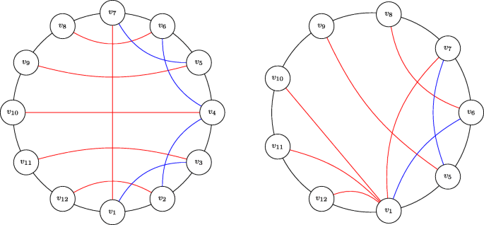

  

  Left: Instance (G₂,L₂) from the lower bound construction in Lemma 4. Red links define an optimal solution. Right: If the algorithm in the first phase picks and contracts the crossing links {(v₁,v₃),(v₂,v₄)}, this is the obtained CacAP instance

• For each $i=1,\dots , \frac {n}{2}-1$, (v_i+ 1,v_n+ 1−i) ∈ L_k;

• For each $i=1,\dots , \frac {n}{6}$, (v_{3(i− 1)+ 1},v_{3(i− 1)+ 3}) ∈ L_k and (v_{3(i− 1)+ 2},v_{3(i− 1)+ 4}) ∈ L_k;

Notice that the first and second set of links define a feasible solution of size $\frac {n}{2}$, hence being optimal: if we remove any two edges of the cycle, then we are either satisfying the corresponding cut via $(v_{1}, v_{\frac {n}{2}+1})$, or one side of the partition is contained in either $\{v_{2}, \dots , v_{\frac {n}{2}}\}$ or in $\{v_{\frac {n}{2}+2}, \dots , v_{n}\}$ but the links selected form a matching between those sets.

We will now prove that there exists a sequence of choices performed by our algorithm that outputs a solution of size $\frac {5n}{6}-1$, which implies that the approximation ratio is at least $\frac {5}{3} - \frac {2}{n}$ and this value approaches $\frac {5}{3}$ as k goes to infinity. Notice first that the pair of links $\{(v_{1},v_{3}), (v_{2},v_{4})\} \subseteq L_{k}$ is crossing, and hence the algorithm can include them in the solution in the first round (and finish the round). Furthermore, after these links are contracted no link becomes external as the new cactus instance consists of a cycle of length n − 3, and also the links with endpoints v_n,v_n− 1 and v_n− 2 are not part of any pair of crossing links (see Fig. 1 (Right)). If we now iteratively pick all the pairs of crossing links $\{(v_{3(i-1)+1},v_{3(i-1)+3}), (v_{3(i-1)+2},v_{3(i-1)+4})\} \subseteq L_{k}$, $i=2,\dots , \frac {n}{6}$, after $\frac {n}{6}$ rounds we end up with a cycle of length $\frac {n}{2}$ without crossing links, and the algorithm must now take the remaining $\frac {n}{2}-1$ links to complete the solution. Thus, the size of the computed solution is $2\cdot \frac {n}{6} + \frac {n}{2}-1 = \frac {5}{6}n - 1$, proving the claim. □

3.2 A $\left (\frac {3}{2}+\varepsilon \right )$-approximation

The family of instances from Lemma 4 suggests that “short” crossing pairs of links, although being locally profitable, may enforce the algorithm to take expensive decisions in the end. In this section we present a more involved $\left (\frac {3}{2}+\varepsilon \right )$-approximation for CycAP that tries to avoid this kind of situation. Like in the previous algorithm, there is a certain kind of links that we want to iteratively add to our solution in a first phase, and in this case such links correspond to external links and long links, which are defined as follows.

Definition 5

The length of an internal link (u,v) is the length of the shortest path between u and v in the corresponding cycle. For a given parameter 0 < ε < 1, an internal link is called long if its length is at least $\frac {1}{\varepsilon }$, and short otherwise.

Our algorithm consists of the following two main phases. In the first phase, we iteratively check if there exists a long (internal) link ℓ. Otherwise, we check if there exists an external link ℓ. In both cases, we add ℓ to the solution under construction and contract it. Observe that contracting links does not create new long links, hence we will first select a set L_long of long links, and then a set L_ext of external links. After exhausting the previous choices, we move to the second phase. Here we are left with an instance where all links are short and internal, so we can solve independently the sub-instance induced by each cycle. We refer to this algorithm as long-first. This second stage can be solved efficiently, due to the lack of long links, by means of the following lemma.¹

Lemma 5

Given a CycAP instance, there exists an algorithm that returns the optimal solution in time $\text {poly}(n)\cdot 2^{O(h_{\max \limits }^{2})}$, where $h_{\max \limits }$ is the maximum length among the links.

Let L_short be the collection of edges obtained in the second stage. The final solution is L_long ∪ L_ext ∪ L_short.

Theorem 3

The long-first algorithm is a $(\frac {3}{2}+\varepsilon )$-approximation algorithm for CycAP.

Proof

The running time of the algorithm is upper-bounded by $\text {poly}(n) 2^{O(1/\varepsilon ^{2})}$. Consider next the approximation factor. Note first that |L_long|≤ εn. Indeed, contracting a long link always increases the number of cycles in the cactus by one without decreasing the number of edges, and all these cycles always have size at least 1/ε, so there are at most εn of them. Similarly to Theorem 2, we have that |OPT|≥|L_short| and $|\text {OPT}|\ge \frac {n}{2}$.

If $|L_{\text {long}}|+|L_{\text {ext}}|+|L_{\text {short}}|\leq \frac {(3+2\varepsilon )n}{4}$ then we already have a $\left (\frac {3}{2}+\varepsilon \right )$-approximation as $|\text {OPT}|\geq \frac {n}{2}$. Otherwise, since the contraction of each external link reduces the number of nodes by at least 2 and the contraction of any other link reduces the number of nodes by at least 1, we have that |L_long| + 2|L_ext| + |L_short|≤ n. So $|L_{\text {ext}}|\leq n-\frac {(3+2\varepsilon )n}{4}=\frac {(1-2\varepsilon )n}{4}$ and hence $|L_{\text {ext}}|+|L_{\text {long}}|\leq \frac {n+2\varepsilon n}{4}\le \left (\frac {1}{2} + \varepsilon \right )|\text {OPT}|$. Since |OPT|≥|L_short|, we have that in this case the size of the solution is also at most $(\frac {3}{2}+\varepsilon )|\text {OPT}|$, concluding the proof. □

Remark 1

By replacing ε with $1/\sqrt {\log n}$ in the above construction, we can obtain a slightly improved approximation factor of 3/2 + o(1) which still runs in polynomial time.

It remains to prove Lemma 5. To do this, we need some more notations. Given a link ℓ = (u,v), we say that the edges of the shortest path between u and v in the cycle are covered by ℓ (in case of multiple shortest paths we choose the one going from u to v in counter-clockwise order along the cycle). Given an edge e of the cycle, we define the cut-neighborhood of e, namely $\mathcal {N}(e)$, as the $2h_{\max \limits }-1$ edges that are closest to e, e included. We also define $\mathcal {N}_{L}(e)$ as the set of links in L covering at least one edge from $\mathcal {N}(e)$.

Notice that in any feasible solution to a CycAP instance, at most one edge of the cycle is not covered: if it is not the case, then the cut defined by two uncovered edges is not satisfied as any link satisfying the cut would cover one of these two edges. We can use this observation to characterize the feasibility of a solution in terms of the cut-neighborhoods.

Lemma 6

Consider a CycAP instance and let A be a set of links such that every edge of the cycle is covered by some link in A. A is feasible iff for each edge e, all the $\{e,e^{\prime }\}$-cuts, where $e^{\prime }\in \mathcal {N}(e)$, are satisfied.

Proof

If A is feasible then the required properties are clearly satisfied since every cut is satisfied. On the other hand, suppose that A satisfies that every edge is covered by some link in A and the $\{e,e^{\prime }\}$-cuts are satisfied for every edge e and $e^{\prime }\in \mathcal {N}(e)$. Consider a pair of edges $\{e,e^{\prime }\}$ such that $e^{\prime }\notin \mathcal {N}(e)$. By definition of $\mathcal {N}(e)$ there is no link in A covering both edges at the same time, and as e is covered by some link, this link satisfies the $\{e,e^{\prime }\}$-cut. This implies that A is feasible as every cut is satisfied. □

This lemma is useful as it implies that, given an edge e and a set of links S, we can optimally complete S in order to satisfy every $\{e,e^{\prime }\}$-cut in time $2^{O(h_{\max \limits }^{2})}$ just by guessing the subset of links from $\mathcal {N}_{L}(e)$ that must be added, which are $O(h_{\max \limits }^{2})$ only. Now we proceed to present the proof.

Proof Proof of Lemma 5

Let us assume that we deal with instances of CycAP such that there exists an optimal solution where every edge is covered by some link. If it is not the case, as there may be only one uncovered edge, we can guess this edge and contract it; this leads to an equivalent instance of the problem where we can require that the optimum solution covers all the edges. We say that an edge e is satisfied by a set of links A if it is covered by some link in A and furthermore every $\{e,e^{\prime }\}$-cut is satisfied by A. In particular A is a feasible solution for the problem iff it satisfies all the edges.

We next design a dynamic programming algorithm to compute a minimum cardinality feasible solution. Let us name the nodes v₁,v₂,...,v_n in counter-clockwise order starting from some arbitrary node v₁, and let the edges be e_i = (v_i,v_i+ 1) for each $i=1,\dots ,n$ (assuming v_n+ 1 = v₁).

For each edge e_i and $S\subseteq \mathcal {N}_{L}(e_{i})$, we define a cell T[i][S] which will correspond to a set $S^{\prime }$ of links of smallest cardinality such that for each $j\in \{1,\dots ,i\}$, e_j is satisfied by $S^{\prime }$, subject to $S\subseteq S^{\prime }$. It is then sufficient to return T[n][∅].

We initialize the table by computing T[1][S] for each set $S\subseteq \mathcal {N}_{L}(e_{1})$, which can be done by guessing how to complete S in order to satisfy e₁ with links from $\mathcal {N}_{L}(e_{1})$. Then, for each i ≥ 2 and $S\subseteq \mathcal {N}_{L}(e_{i})$, in order to fill the cell T[i][S], we consider all the possible subsets $A\subseteq \mathcal {N}_{L}(e_{i})$ such that $S(A):=T[i-1][(S\cup A)\cap \mathcal {N}_{L}(e_{i-1})] \cup (S\cup A)$ satisfies e_i. Among them we select a set A^∗ that minimizes |S(A)|, and we set T[i][S] = S(A^∗) (see Fig. 2 for a sketch).

Fig. 2

Depiction of an iteration of the DP from Lemma 5, where we are currently at edge e_i. Left: Green links correspond to S and at this point we must decide which extra links to add to S in order to satisfy the edges $e_{1},\dots ,e_{i}$. Right: This computation is done by looking at a proper previous cell in the table (orange links) which contains S and satisfies $e_{1},\dots ,e_{i-1}$, and then add the extra required links A^∗ (red links) in order to satisfy e_i too

The correctness of the computation follows by a simple induction on i. The table can be filled in total time $\text {poly}(n) \cdot 2^{O(h_{\max \limits }^{2})}$, plus an extra factor n from the initial guessing of an uncovered edge (that is contracted). □

We complement Theorem 3 with an asymptotically matching lower bound.

Lemma 7

The approximation ratio of the long-first algorithm is at least $\frac {3}{2}$.

Proof

Consider the following construction: for each $k> \frac {1}{2\varepsilon }$ consider an instance (G_k,L_k) of CycAP defined by a cycle of n = 4k nodes (assume that the cycle is defined by the order of the nodes $v_{1},v_{2}, \dots , v_{4k}$) and the following set of links (see Fig. 3 (Left)):

• For each $i=1,\dots , \frac {n}{2}-1$, (v_i+ 1,v_n+ 1−i) ∈ L_k;

  Fig. 3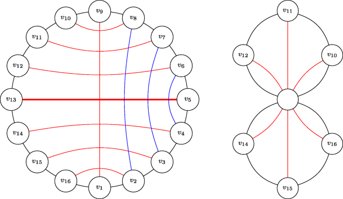

  

  Left: Instance (G₄,L₄) from the lower bound construction in Lemma 7. An optimal solution is defined by red links. Right: If the algorithm picks first the thick red link (which is long) and then the links which become external (blue links and (v₁,v₉)) we obtain this subinstance without crossing pairs of links

• $(v_{1}, v_{\frac {n}{2}+1}) \in L_{k}$;

• For each $i=1,\dots , \frac {n}{4}-1$, $(v_{i+1},v_{\frac {n}{2}+1-i}) \in L_{k}$.

As argued in Lemma 4, the first and second set of links define an optimal solution of size $\frac {n}{2}$. We will now prove that there exists a sequence of choices performed by our algorithm that outputs a solution of size $\frac {3n}{4}-1$, which implies that the approximation ratio is at least $\frac {3}{2} - \frac {2}{n}$ and this value approaches $\frac {3}{2}$ as k goes to infinity. Notice first that the link $(v_{\frac {n}{4}+1}, v_{\frac {3n}{4}+1})\in L_{k}$ has length $2k>\frac {1}{\varepsilon }$ and hence it is long so the first stage of the algorithm can include it in the solution. After doing that, the second and third set of links become external and thus the algorithm will include them in the solution. Once all these links are included and contracted, we get a cactus consisting of two cycles of $\frac {n}{4}$ nodes each and without crossing links (see Fig. 3 (Right)). Hence, the algorithm must pick all the remaining links to complete the solution. The size then of this solution is $\frac {n}{4} + 1 + 2\left (\frac {n}{4}-1\right ) = \frac {3n}{4}-1$. □

4 LP Relaxations for CycAP

We start by lower-bounding the integrality gap of the standard cut LP for CycAP.

Lemma 8

The standard cut LP for CycAP has integrality gap at least 2.

Proof

Consider a cycle of size k and, for each edge, a parallel link. The optimum integral solution has size k − 1, while setting each variable to $\frac {1}{2}$ gives a feasible fractional solution of cost $\frac {k}{2}$. □

This shows that the standard cut LP is not strong enough even for instances without crossing nor long links, cases that we can handle optimally via combinatorial algorithms. We next present a stronger LP that exploits a more general set of constraints.

Let (G = (V,E),L) be a CycAP instance and $S\subseteq E$. We define the S-reduced instance (G_S,L_S) as follows: We contract the edges of E ∖ S, obtaining a cycle with |S| edges which defines G_S, and the set of links L_S will correspond to the images of L. Notice that there is a one-to-one relation between L_S and the links in L which satisfy some cut defined by a pair of edges from S. We denote by OPT_S the optimal solution for the instance (G_S,L_S)². The following lemma characterizes the feasibility of a solution.

Lemma 9

Given an instance (G,L) of CycAP, a solution $A\subseteq L$ is feasible iff for every $S\subseteq E$ it holds that |A ∩ L_S|≥|OPT_S|.

Proof

Suppose that there exists $S\subseteq E$ such that |A ∩ L_S| < |OPT_S|. This means that A ∩ L_S is not a feasible solution for (G_S,L_S) and hence there exist two edges e_i,e_j ∈ S such that no link in A ∩ L_S satisfies the {e_i,e_j}-cut. As the remaining links in A ∖ L_S also do not satisfy the cut by definition, this cut remains unsatisfied in the original instance, implying that A is not feasible.

On the other hand, suppose that A satisfies the claimed property for every set S. If we consider just sets S consisting of two edges this is exactly the characterization of feasibility shown in Observation1, implying that A is feasible. □

This implies that we can add the constraint ${\sum }_{\ell \in L_{S}}{x_{\ell }} \ge |\text {OPT}_{S}|$ for $S\subseteq E$. Unfortunately there is an exponential number of such constraints and most of them require to compute |OPT_S| for large instances. However, if we restrict ourselves to sets of edges having constant size, we get an LP formulation with polynomially many constraints that can be written in polynomial time. We call this LP the k-edge-cut LP for a given constant $k\in \mathbb {N}$, which is similar in spirit to the bundle-LP for TAP introduced by Adjiashvili [1].

$$\begin{array}{rll} \min & \sum\limits_{\ell \in L}{x_{\ell}}& (k\text{-edge-cut LP}) \\ s.t. & \sum\limits_{\ell\in L_{S}}{x_{\ell}} \ge |\text{OPT}_{S}| & \forall S\subseteq E, |S|\le k \\ & 0\leq x_{\ell}\leq 1 & \forall \ell \in L \end{array}$$

Notice that for k = 2 this is exactly the standard cut LP. Now we will prove some properties of this relaxation and bound its integrality gap.

Lemma 10

Given ε > 0, for $k=\frac {1}{\varepsilon ^{2}}$ the k-edge-cut LP restricted to instances with links of length at most $\frac {1}{\varepsilon }$ has integrality gap at most (1 + 2ε).

Proof

We will assume w.l.o.g. that the set of links L contains every possible link of length 1. If it is not the case, let us include them obtaining a new set of links $L^{\prime } \supseteq L$. The optimal LP value can only decrease while the size of the optimal solution cannot decrease, implying that the integrality gap can only increase due to this operation. To see this last fact, assume by contradiction that there exists a solution $\text {OPT}^{\prime }$ for the new instance having strictly smaller size than OPT. Consider now a solution S consisting of $\text {OPT}^{\prime }\cap L$ plus a minimal set of links from L that makes S feasible (this is possible since the instance admits a feasible solution). If we in parallel iteratively contract the common links in S and $\text {OPT}^{\prime }$ we arrive to the same CacAP instance, but now the remaining links from $\text {OPT}^{\prime }$ have length 1 and the contraction of each of them reduces the number of nodes in the instance by exactly one node while the contraction of the remaining links in S reduces the number of nodes by at least 1. Thus $|S|\le |\text {OPT}^{\prime }|$ which is not possible since $S\subseteq L$.

Let X = (x_ℓ)_ℓ∈L be an optimal solution for the k-edge-cut LP. We will construct an integral feasible solution of size at most $(1+\varepsilon ) {\sum }_{\ell \in L}{x_{\ell }}$. To do so, we will partition the cycle into disjoint intervals as follows: We will first define an interval of size k (which we will call a long interval) and then an interval of size $\frac {1}{\varepsilon }$ (which we will call a short interval), and then continue with this procedure until it is not possible to continue. If in the end there are at most $\frac {1}{\varepsilon }$ edges we define a last short interval consisting of these remaining edges, otherwise we define a short interval consisting of the last $\frac {1}{\varepsilon }$ edges and a long interval consisting of the remaining edges (which will have size at most k). The number of short intervals is upper bounded by $1+\left \lfloor \frac {n}{1/\varepsilon ^{2}+1/\varepsilon }\right \rfloor \leq 1+\frac {\varepsilon ^{2} n}{1+\varepsilon }\leq \varepsilon ^{2} n$ assuming w.l.o.g. that n is lower bounded by a large enough constant.

Notice that ${\sum }_{\ell \in L}{x_{\ell }} \ge n/2$ by a simple averaging argument over the n constraints corresponding to all the pairs of consecutive edges: every link appears in exactly two such constraints and the right-hand side of each constraint is 1. Since the total number of links of length 1 having both endpoints in a short interval is at most $\varepsilon ^{2} n \cdot \frac {1}{\varepsilon } = \varepsilon n \le 2 \varepsilon {\sum }_{\ell \in L}{x_{\ell }}$, we can add them to our solution at a negligible cost.

Consider now the set of long intervals $S_{1}, S_{2}, \dots , S_{T}$. Notice that no link has endpoints in different long intervals, and hence the LP constraints associated to such intervals do not share common variables. This implies that ${\sum }_{\ell \in L}{x_{\ell }} \ge {\sum }_{i=1}^{T}{|\text {OPT}_{S_{i}}|}$. Our feasible solution will consist of all the links of length 1 with both endpoints in a short interval plus the optimal solutions $\text {OPT}_{S_{i}}$ for each long interval S_i. As argued before, the size of this solution is at most $(1+2\varepsilon ) {\sum }_{\ell \in L}{x_{\ell }}$ and the feasibility of the solution follows since every $\{e,e^{\prime }\}$-cut where e is in a short interval is satisfied by a link of length 1, while the remaining cuts are satisfied by the links computed optimally. □

Lemma 11

Given ε > 0, for $k=\frac {1}{\varepsilon ^{2}}$ the k-edge-cut formulation has integrality gap at most (1 + 4ε) restricted to instances without crossing pairs of links.

Proof

Let X = (x_ℓ)_ℓ∈L be an optimal solution for the k-edge-cut LP. Suppose that the instance does not contain links of length at least $\frac {1}{\varepsilon }$, then we can conclude the claim thanks to Lemma 10. Otherwise, we will pick any link of length at least $\frac {1}{\varepsilon }$ and contract it, obtaining a CacAP instance consisting of two cycles without external links (as there are no crossing links), both of size at least $\frac {1}{\varepsilon }$. If any cycle still contains some long link, we iterate this procedure. Let L_long be the set of long links we picked during this procedure and $C_{1}, C_{2}, \dots , C_{T}$ be the set of cycles at the end. By the same argument as in Theorem 3, we have that $|L_{\text {long}}|\le \varepsilon n \le 2\varepsilon {\sum }_{\ell \in L}{x_{\ell }}$.

Applying Lemma 10 to each cycle, we obtain a feasible solution of size at most $(1+2\varepsilon ){\sum }_{i=1}^{T}{\text {OPT}_{\text {LP}_{i}}} + |L_{\text {long}}|$, where LP_i is the k-edge-cut LP defined by each cycle C_i and its internal links. As there are no external links, the sum of the previous LP solutions is the optimal solution for the following LP:

$$ \begin{array}{rlr} \min & \sum\limits_{\ell \in L\setminus L_{\text{long}}}{x_{\ell}}& \\ s.t. & \sum\limits_{\ell\in L_{S}}{x_{\ell}} \ge |\text{OPT}_{S}| & \forall i\in\{1,\dots,T\}, \forall S\subseteq E(C_{i}), |S|\le \frac{1}{\varepsilon^{2}} \\ & 0\leq x_{\ell}\leq 1 & \forall \ell \in L\setminus L_{\text{long}} \end{array} $$

The set of constraints of this LP is a subset of the constraints of the original LP as links in L_long do not appear in these constraints and the set of variables is a subset of the original one. Thus we have ${\sum }_{i=1}^{T}{\text {OPT}_{\text {LP}_{i}}}\le {\sum }_{\ell \in L}{x_{\ell }}$, and then we can conclude that the constructed solution has size at most $(1+4\varepsilon ){\sum }_{\ell \in L}{x_{\ell }}$. □

Following the proof of Theorem 3 plus the previous results we can get the following bound on the integrality gap for general instances of CycAP.

Corollary 1

For any ε > 0, the integrality gap of the k-edge-cut LP for $k=\frac {1}{\varepsilon ^{2}}$ is at most $\frac {3}{2}+O(\varepsilon )$.

Proof

Let X = (x_ℓ)_ℓ∈L be an optimal solution for the k-edge cut LP and consider the output of the $\left (\frac {3}{2}+\varepsilon \right )$-approximation from Section 3.2 decomposed into L_long, L_ext and L_short as in the proof of Theorem 3. As argued before, we know that ${\sum }_{\ell \in L}{x_{\ell }}\ge \frac {n}{2}$ and analogously to the proof of Lemma 11 we have that $|L_{\text {short}}|\le (1+2\varepsilon ){\sum }_{\ell \in L}{x_{\ell }}$. Hence essentially the same analysis as in Theorem 3 provides the same bound of 3/2 + O(ε) up to an extra (1 + ε) factor. □

5 Hardness of Approximation

In the following two sections we discuss the hardness of approximation for WCycAP and CycAP, respectively.

5.1 Hardness of Approximation for WCycAP

We now provide an approximation preserving reduction from WCacAP to WCycAP. Note that finding a better-than-2-approximation for WCacAP is at least as hard as finding such an approximation for WTAP, a big open problem in the area. Therefore our reduction shows that achieving a similar result for WCycAP is a very hard task as well.

Theorem 4

Given an instance A of WCacAP, it is possible to construct in polynomial time an instance B of WCycAP (whose only possibly new weight value is 0) such that any feasible solution to A can be mapped in polynomial time into a feasible solution to B of the same cost and vice versa.

To prove Theorem 4 we make use of the “inverse” of the contraction of a link, which we call an expansion: Consider a WCacAP instance with a node v with degree greater than 2. An expansion of v will consist of taking two cycles containing v and replacing them by the Eulerian tour that traverses them starting from v. Every node appears exactly once except for v which appears twice, for which we create two copies: v₁ the starting node and v₂ the intermediate one. The links originally incident to v are replaced by links of the same cost incident to v₁, and we also add a link of cost zero between v₁ and v₂ (see Fig. 4 for an example). The two main properties of this procedure are that: (1) the contraction of a link created by an expansion brings back the graph to the original state and (2) v is replaced by v₁ and v₂, which have degree $\deg (v)-2$ and 2, respectively.

Fig. 4

Depiction of an expansion applied to node v in the left graph considering the cycles to the left and right of v. Dashed edges correspond to links and the highlighted link in the middle graph corresponds to the extra link of cost zero added by the expansion. The right graph is the final WCycAP instance formed by another expansion on the middle graph

Proof Proof of Theorem 4

At high level our proof works as follows. We will build in polynomial time a chain of WCacAP instances (G₁,L₁),…,(G_k,L_k), with the following properties: (i) (G₁,L₁) is the input instance and G_k is a cycle; (ii) (G_i+ 1,L_i+ 1), i = 1,…,k − 1, is obtained from (G_i,L_i) via precisely one expansion (so G_i+ 1 contains precisely one cycle less than G_i, and precisely one new link ℓ_i+ 1 of cost zero); (iii) a feasible solution to (G_i,L_i), i = 1,…,k − 1, can be turned in polynomial time into a feasible solution to (G_i+ 1,L_i+ 1) of the same cost and vice versa. The above properties together trivially imply the claim.

Given (G_i,L_i), we proceed as follows. Consider any node v ∈ G_i of degree at least 4, and let C₁ and C₂ be any two cycles incident to v (that must exist). We apply an expansion to node v w.r.t. C₁ and C₂, hence creating a new link ℓ_i+ 1 of cost zero. Properties (i) and (ii) follow immediately by construction. Observe that (G_i,L_i) can be obtained from (G_i+ 1,L_i+ 1) by contracting ℓ_i+ 1. Hence property (iii) follows directly from Lemma 1. In more detail, given a feasible solution A_i+ 1 to (G_i,L_i), we first add ℓ_i+ 1 to A_i+ 1 (that keeps the solution feasible, and does not change its cost). By Lemma 1, A_i := A_i+ 1 ∖ ℓ_i+ 1 is a feasible solution to (G_i,L_i) of the same cost. Vice versa, given a feasible solution A_i to (G_i,L_i), A_i+ 1 := A_i ∪ ℓ_i+ 1 is a feasible solution to (G_i+ 1,L_i+ 1) of the same cost. □

5.2 Hardness of Approximation for CycAP

In this section we prove that CycAP is APX-hard via a reduction from a restricted case of 3-Dimensional Matching (3DM). In the general version of 3DM we are given three disjoint sets W,X and Y having equal cardinality p and a set of m hyperedges $H\subseteq W\times X \times Y$. A (3D) matching is a subset $M\subseteq H$ such that each element of W ∪ X ∪ Y belongs to at most one hyperedge in M, and this matching is perfect if |M| = p. Notice that in a perfect matching M each element of W ∪ X ∪ Y belongs to precisely one hyperedge. The goal is to determine whether a perfect matching exists. We will consider the special case 3DM-K, $K\in \mathbb {N}$, where we add the constraint that each element from W ∪ X ∪ Y appears in at most K hyperedges. The following result will help us to conclude our final claim.

Theorem 5 (Petrank 30)

For some fixed ε₀ > 0, it is NP-hard to distinguish whether an instance of 3DM-5 with |W| = |X| = |Y | = q has a perfect matching (of size q) or every matching has size at most (1 − ε₀)q.

The proof of the following theorem is similar in spirit to the proof of NP-hardness for WTAP due to Frederickson and JáJá [15] and the extension presented by Kortsarz et al. [23]. In the first reduction the authors start from an instance A of 3DM with 3p nodes and m hyperedges, and build a WTAP instance B such that: A has a feasible solution (with p hyperedges) iff B has a feasible solution with p + m links. By duplicating the edges in B, one obtains a CacAP instance C with exactly the same property over some cactus G. Our main idea is to turn C into an instance D of CycAP by constructing an Euler tour $G^{\prime }$ out of G and shortcutting some nodes. However, we need to carefully choose the ordering in the Euler tour in order to preserve a mapping between the feasible solutions of C and D. By following the refined approach from the second reduction, we will show that it is hard to distinguish solutions with a gap depending on the maximum degree in the instance and then use Theorem 5 to conclude the following result.

Theorem 6

For some fixed ε > 0, it is NP-hard to approximate CycAP within a factor 1 + ε.

Construction of the Instance

Let $H\subseteq W\times X\times Y$ be an instance of 3DM with |H| = m, $W=\{w_{1},\dots ,w_{p}\}, X=\{x_{1},\dots ,x_{p}\}$ and $Y=\{y_{1},\dots ,y_{p}\}$. We will define an instance (G = (V,E),L) of CycAP where nodes are placed on the cycle in the order as they appear below in counterclockwise direction (see Fig. 5 for a depiction of the instance):

• For each node x_i ∈ X we define a node x_i;

• For each node y_i ∈ Y we define a node y_i;

• Let H(w_i) denote the hyperedges in H containing w_i ∈ W. For each hyperedge h ∈ H(w_i) we define two nodes, namely h_X and h_Y (hyperedge nodes). These nodes are added to the cycle in the following order. For each $i \in \{1, \dots , p\}$, we add first nodes h_X corresponding to hyperedges in H(w_i) (in some arbitrary order) and then the corresponding nodes h_Y respecting the same order used before. We will denote the first set of nodes by H_X(w_i), and the second set by H_Y(w_i).

The set of links L is defined as follows:

• For each hyperedge h ∈ H we add the link (h_X,h_Y);

• For each hyperedge h ∈ H and a node x ∈ X, we add the link (h_X,x) iff x ∈ h;

• For each hyperedge h ∈ H and a node y ∈ Y, we add the link (h_Y,y) iff y ∈ h.

Fig. 5

Example of the construction in Theorem 6. Red links correspond to hyperedge h⁽²⁾ = (w₁,x₂,y₁) and green links join the copies of the hyperedges

Lemma 12

If the 3DM instance H contains a 3D matching M with p hyperedges then the CycAP instance (G,L) constructed as above admits a solution A of size p + m.

Proof

Suppose that H contains a 3D matching M of size p. We build a solution A to (G,L) as follows: For each hyperedge h = (w,x,y) ∈ M we add to A the links (h_X,x) and (h_Y,y). Also, for each hyperedge h ∈ H ∖ M we add the link (h_X,h_Y) to A. Observe that the total number of links in A is 2p + (m − p) = p + m.

Let us show that A is a feasible solution. By Observation 1, it is sufficient to consider any pair of edges {e₁,e₂}, and show that there exists some link ℓ ∈ A satisfying the corresponding {e₁,e₂}-cut. Let us denote by $S^{\prime }$ and $S^{\prime \prime }$ the sets of nodes induced by the cut. Let H_X (resp., H_Y) be the collection of nodes of type h_X (resp., h_Y). We make the following case distinction: Suppose first that e₁ is incident to two nodes in X or e₁ = (x_p,y₁) (the case e₁ being incident to two nodes in Y is symmetric). We distinguish the following 3 subcases depending on e₂:

• 1. Suppose e₂ is incident to at least one node in X ∪ Y. Then one of the sets in the cut, say $S^{\prime \prime }$, contains all the hyperedge nodes while $S^{\prime }$ contains at least one node in z ∈ X ∪ Y. By construction each node in X (resp. Y) is adjacent to some node in H_X (resp., in H_Y). Thus this cut is satisfied.

• 2. Suppose e₂ is not incident to any node in H_Y(w_p). Then one of the sets in the cut, say $S^{\prime }$, contains completely Y, while $S^{\prime \prime }$ contains H_Y(w_p). By construction, for h = (w_p,x,y) ∈ M, ℓ = (h_Y,y) ∈ A, hence this cut is satisfied.

• 3. Suppose e₂ is incident to some node in H_Y(w_p). Then one of the sets in the cut, say $S^{\prime \prime }$, contains H_X while the other set contains at least one node x from X. Again by construction, for h = (w,x,y) ∈ M, ℓ = (h_X,x) ∈ A. Hence this cut is satisfied.

Suppose on the other hand that e₁ and e₂ are incident to at least one hyperedge node. Notice that one of the sets in the cut, say $S^{\prime }$, contains X ∪ Y. We distinguish the following 2 subcases:

• 1. If $S^{\prime \prime }$ contains entirely H_X(w) or H_Y(w) for some w ∈ W, then for h = (w,x,y) ∈ M, (h_X,x) or (h_Y,y) is contained in A and the cut is satisfied.

• 2. In the remaining case we prove that the following claim holds: There exists an hyperedge h such that $h_{X}\in S^{\prime }$ and $h_{Y}\in S^{\prime \prime }$.

  Suppose by contradiction that for every hyperedge h both h_X and h_Y belong to the same side of the considered cut. Let w_i be such that either H_X(w_i) or H_Y(w_i) has non-empty intersection with both sides of the cut. Note that such w_i must exist, otherwise there would exist w_j such that $S^{\prime \prime }$ contains either H_X(w_j) or H_Y(w_j) completely which was already covered by the previous case. Assume w.l.o.g. that $H_{X}(w_{i}) = \{{h_{X}^{1}},\dots ,{h_{X}^{q}}\}$ is the considered set with elements sorted in counterclockwise direction. Since ${h_{X}^{1}}$ and ${h_{Y}^{1}}$ are on the same side of the partition and H_X(w_i) is not fully contained in any side of the partition, it must hold that one set of the partition is properly contained in H_X(w_i). Then any node inside that set has its copy on the other side of the partition. This is in contradiction with the assumption.

  Let h be an hyperedge as in the previous claim. We are either adding to the solution the link that joins both copies of h (i.e. the case when h∉M) and the proof is finished, or we are adding the two links joining the two copies of h to elements in X and Y (i.e. the case when h ∈ M). Since X ∪ Y is contained in $S^{\prime }$ and both copies of h are in different sides of the partition, one of the links satisfies the cut.

□

For any z ∈ W ∪ X ∪ Y in a 3DM instance, let $\deg (z)$ be the number of hyperedges in H containing z. Let also Δ denote the maximum degree of the instance, i.e., $\varDelta =\max \limits _{z\in W\cup X\cup Y}{\deg (z)}$. By following an analogous approach to the one from Kortsarz et al. [23], we can prove that even instances with a gap can be mapped.

Lemma 13

If the CycAP instance (G,L) constructed as above admits a solution A with |A|≤ (1 + ε)(p + m), then the 3DM instance H contains a 3D matching M with |M|≥ p − (2 + 10Δ)(p + m)ε.

Proof

Let A be a feasible solution to (G,L) with |A|≤ (1 + ε)(p + m). Note that G contains 2(p + m) nodes and the links must form an edge cover (otherwise the resulting graph would not be 3-edge-connected). Call a node permissible if it is adjacent to exactly one link in A and impermissible otherwise. Let V_perm and V_imperm be the set of permissible and impermissible nodes respectively. We will first prove that the number of impermissible nodes is upper bounded by 2ε(p + m). In fact, if $\deg _{A}(v)$ denotes the number of links in A incident to v, we have that

$$2|A| = \sum\limits_{v\in V}{|\deg_{A}(v)|} = \sum\limits_{v\in V_{\text{perm}}}{\deg_{A}(v)} + \sum\limits_{v\in V_{\text{imperm}}}{\deg_{A}(v)} \ge |V_{\text{perm}}| + 2|V_{\text{imperm}}|$$

where the last inequality comes from the fact that impermissible nodes are adjacent to at least two links. Since |A|≤ (1 + ε)(p + m), and |V_perm| + |V_imperm| = 2(p + m), we can conclude the claim.

We will now compute a set $M^{\prime }$ which is almost a matching. We initialize $M^{\prime }=\emptyset$ and then, iteratively for $j=1,\dots , p$, we try to add an hyperedge to $M^{\prime }$ as follows: if x_j is permissible, then it is adjacent to one node $h_{x}^{(j)} \in H_{X}$ (let us assume $h_{x}^{(j)}\in H_{X}(w_{i})$); if both $h_{x}^{(j)}$ and its copy $h_{y}^{(j)}\in H_{Y}(w_{i})$ are permissible, then $h_{y}^{(j)}$ is adjacent to one node y_k. If y_k is permissible, then we add (w_i,x_j,y_k) to $M^{\prime }$. Notice that hyperedges added by this procedure are indeed in H by construction. Our claim is that $|M^{\prime }|\ge p-2\varDelta (p+m)\varepsilon$. Actually, if x_j, $h_{x}^{(j)}$ or $h_{y}^{(j)}$ are impermissible, then only one iteration fails (the one indexed by j). If y_k is impermissible then it can cause at most Δ iterations to fail, since it can be connected to at most Δ nodes in H_Y. If we denote by n_y the number of impermissible nodes y_k involved in the procedure, then the number of iterations that fail is at most (2ε(p + m) − n_y) + n_yΔ. Since n_y ≤ 2ε(p + m) (the total number of impermissible nodes), the number of iterations that fail is at most 2Δ(p + m)ε, proving the claim.

By construction, hyperedges in $M^{\prime }$ have different elements from X and Y but elements from W might be repeated. Thus, for every w_i belonging to more than one hyperedge in $M^{\prime }$, we remove from $M^{\prime }$ all but one of such hyperedges, obtaining $M^{\prime \prime }$ which is now a matching. Let $\mu =p-|M^{\prime \prime }|$ be the number of vertices w_i not appearing in any hyperedge of $M^{\prime }$ (equivalently of $M^{\prime \prime }$). Since $|M^{\prime }|-|M^{\prime \prime }| \le p-|M^{\prime \prime }|=\mu$, we can find a lower bound on the size of $M^{\prime \prime }$ by bounding above μ. We indeed claim that μ ≤ (2 + 8Δ)(p + m)ε.

Let $L^{\prime }$ be the links in L of the form $(x_{j},h_{X}^{(j)})$ and $(y_{k},h_{Y}^{(j)})$ where $h_{x}^{(j)}$ corresponds to a hyperedge $(w_{i}, x_{j}, y_{k})\in M^{\prime }$ and $h_{y}^{(j)}$ corresponds to its copy. We have that $|L^{\prime }| = 2|M^{\prime }| \ge 2p-4\varDelta (p+m)\varepsilon$, hence

$$|A\setminus L^{\prime}| \le (1+\varepsilon)(p+m) - 2p+4\varDelta(p+m)\varepsilon = m-p+(1+4\varDelta)(p+m)\varepsilon.$$

Consider on the other hand the μ nodes w_i which are not intersected by hyperedges in $M^{\prime }$. Since A is a feasible solution, for each such w_i there must be a link in A connecting H_X(w_i) ∪ H_Y(w_i) and X ∪ Y, because otherwise we could disconnect H_X(w_i) ∪ H_Y(w_i) from the rest of the graph by removing the two edges in the boundary of H_X(w_i) ∪ H_Y(w_i), contradicting the feasibility of A. Notice that these μ links are part of $A\setminus L^{\prime }$. Furthermore, since A is an edge cover, the remaining 2m − 2p − μ nodes in H_X ∪ H_Y untouched by $L^{\prime }$ plus the μ aforementioned links must be incident to some link in A, implying that

$$|A\setminus L^{\prime}| \ge \mu + \frac{2m-2p-\mu}{2} = m-p+\frac{\mu}{2}.$$

Combining both inequalities we get that μ ≤ (2 + 8Δ)(p + m)ε, and hence we conclude that the size of $M^{\prime \prime }$ is at least

$$|M^{\prime}|-\mu \ge p-2\varDelta(p+m)\varepsilon-(2+8\varDelta)(p+m)\varepsilon = p-(2+ 10\varDelta)(p+m)\varepsilon,$$

completing the proof. □

We can now use Lemmas 12 and 13 together with Theorem 5 to conclude the proof of Theorem 6. Notice that in 3DM-5, since Δ = 5, we have that m = |H|≤ 5|W| = 5p.

Proof Proof of Theorem 6

We will show that our reduction presented above is gap-preserving. Specifically, we will show that if H is an instance of 3DM-5 and (G,L) is the corresponding CycAP instance, then

• 1. If H admits a matching of size p, then (G,L) admits a feasible solution of size p + m;

• 2. If H does not admit a matching of size at least p(1 − ε₀), then (G,L) does not admit a feasible solution of size at most $(p+m)(1+\frac {\varepsilon _{0}}{312})$.

The first statement follows directly from Lemma 12, while the second is the contrapositive of Lemma 13 when setting $\varepsilon =\frac {\varepsilon _{0}}{312}$, as in this case we have that p − (2 + 10Δ)(5p + p)ε = p(1 − 312ε) = p(1 − ε₀). □

References

Adjiashvili, D.: Beating approximation factor two for weighted tree augmentation with bounded costs. ACM Transactions on Algorithms, 1549–6325 (2018)
Byrka, J., Grandoni, F., Jabal Ameli, A.: Breaching the 2-Approximation barrier for connectivity augmentation: a reduction to steiner tree. ACM Symposium on Theory of Computing (STOC), 815–825 (2020)
Basavaraju, M., Fomin, F. V., Golovach, P., Misra, P., Ramanujan, M. S., Saurabh, S.: Parameterized algorithms to preserve connectivity. ICALP 2014, 800–811 (2014)
Cheriyan, J., Gao, Z.: Approximating (Unweighted) Tree Augmentation via Lift-and-Project, Part I: Stemless TAP. Algorithmica 80, 530–559 (2018)
Cheriyan, J., Gao, Z.: Approximating (Unweighted) Tree Augmentation via Lift-and-Project, Part II. Algorithmica 80, 608–651 (2018)
Cheriyan, J., Jordán, T., Ravi, R.: On 2-Coverings and 2-Packings of laminar families. ESA 1999, 510–520 (1999)
Cheriyan, J., Karloff, H., Khandekar, R., Könemann, J.: On the integrality ratio for tree augmentation. Oper. Res. Lett. 36, 399–401 (2008)
Cohen, N., Nutov, Z.: A (1 + ln2)-approximation algorithm for minimum-cost 2-edge-connectivity augmentation of trees with constant radius. Theor. Comput. Sci., 67–74 (2013)
Cormen, T. H., Leiserson, C. E., Rivest, R. L., Stein, C.: Introduction to algorithms. Third edition (2009)
Dinitz, E., Karzanov, A., Lomonosov, M.: On the structure of the system of minimum edge cuts of a graph. Studies in Discrete Optimization, 290–306 (1976)
Even, G., Feldman, J., Kortsarz, G., Nutov, Z.: A 1.8 approximation algorithm for augmenting edge-connectivity of a graph from 1 to 2. ACM Trans. Algorithms 5, 21:1–21:17 (2009)
Fiorini, S., Groß, M., Könemann, J., Sanità, L.: Approximating weighted tree augmentation via Chvátal-Gomory cuts. SODA 2018, 817–831 (2018)
Frank, A.: Augmenting graphs to meet edge-connectivity requirements. SIAM J. Discrete Math. 5, 25–53 (1992)
Frank, A.: Connections in combinatorial optimization. Number 38 in Oxford lecture series in mathematics and its applications (2011)
Frederickson, G. N., JáJá, J.: Approximation algorithms for several graph augmentation problems. SIAM J. Comput. 10, 270–283 (1981)
Goemans, M. X., Goldberg, A. V., Plotkin, S., Shmoys, D. B., Tardos, É., Williamson, D.P.: Improved approximation algorithms for network design problems. SODA 1994, 223–232 (1994)
Grandoni, F., Kalaitzis, C., Zenklusen, R.: Improved approximation for tree augmentation: Saving by rewiring. STOC 2018, 632–645 (2018)
Hsu, T.: On four-connecting a triconnected graph. J. Algorithms 35, 202–234 (2000)
Jain, K.: A factor 2 approximation algorithm for the generalized Steiner network problem. Combinatorica 21, 39–60 (2001)
Jordan, T.: On the optimal vertex-connectivity augmentation. J. Combin. Theory 35, 202–234 (1995)
Khuller, S., Thurimella, R.: Approximation algorithms for graph augmentation. J. Algorithms 14, 214–225 (1993)
Knuth, D. E.: Postscript about NP-hard problems. SIGACT News 6, 15–16 (1974)
Kortsarz, G., Krauthgamer, R., Lee, J. R.: Hardness of approximation for Vertex-Connectivity network design problems. SIAM J. Comput. 33, 704–720 (2004)
Kortsarz, G., Nutov, Z.: A Simplified 1.5-Approximation Algorithm for Augmenting Edge-Connectivity of a Graph from 1 to 2. ACM Trans. Algorithms 12, 23:1–23:20 (2015)
Kortsarz, G., Nutov, Z.: Approximating minimum cost connectivity problems. Handbook on Approximation Algorithms and Metaheuristics 35, 202–234 (2007)
Kortsarz, G., Nutov, Z.: LP-relaxations for tree augmentation. APPROX/RANDOM 2016, 13:1–13:16 (2016)
Marx, D., Végh, L.: Fixed-parameter algorithms for minimum-cost edge-connectivity augmentation. ACM Trans. Algorithms 11 (4), 27:1–27:24 (2015)
Nagamochi, H.: An approximation for finding a smallest 2-Edge-Connected subgraph containing a specified spanning tree. Discrete Appl. Math. 126, 83–113 (2003)
Nutov, Z.: On the tree augmentation problem. ESA 2017, 61:1–61:14 (2017)
Petrank, E.: The hardness of approximation: Gap location. Comput. Complex. 4, 133–157 (1994)
Shmoys, D. B.: The design of approximation algorithms. Cambridge (2011)
Végh, L.: Augmenting undirected Node-Connectivity by one. SIAM Journal of Discrete Mathematics, 695–718 (2011)
Watanabe, T., Nakamura, A.: Edge-Connectivity Augmentation problems. J. Comput. Syst. Sci. 35, 96–144 (1987)
Williamson, D. P., Shmoys, D. B.: Algorithms and Complexity. Elsevier, Amsterdam (2011)
Funding
Open Access funding provided by SUPSI - University of Applied Sciences and Arts of Southern Switzerland
Author information
Authors and Affiliations
Corresponding author
Additional information
Publisher’s Note
Springer Nature remains neutral with regard to jurisdictional claims in published maps and institutional affiliations.
This article belongs to the Topical Collection: Special Issue on Approximation and Online Algorithms (2019)
Guest Editors: Evripidis Bampis and Nicole Megow
Partially supported by the SNSF Grant 200021_159697/1, the SNSF Excellence Grant 200020B_182865/1, the National Science Centre, Poland, grant numbers 2015/17/N/ST6/03684, 2015/18/E/ST6/00456 and 2018/28/T/ST6/00366. K. Sornat was also supported by the Foundation for Polish Science (FNP) within the START programme.
Rights and permissions
Open Access This article is licensed under a Creative Commons Attribution 4.0 International License, which permits use, sharing, adaptation, distribution and reproduction in any medium or format, as long as you give appropriate credit to the original author(s) and the source, provide a link to the Creative Commons licence, and indicate if changes were made. The images or other third party material in this article are included in the article's Creative Commons licence, unless indicated otherwise in a credit line to the material. If material is not included in the article's Creative Commons licence and your intended use is not permitted by statutory regulation or exceeds the permitted use, you will need to obtain permission directly from the copyright holder. To view a copy of this licence, visit http://creativecommons.org/licenses/by/4.0/.
About this article
Cite this article
Gálvez, W., Grandoni, F., Jabal Ameli, A. et al. On the Cycle Augmentation Problem: Hardness and Approximation Algorithms. Theory Comput Syst 65, 985–1008 (2021). https://doi.org/10.1007/s00224-020-10025-6
Accepted:
Published:
Issue Date:
DOI: https://doi.org/10.1007/s00224-020-10025-6