
Article Outline
Glossary
Definition of the Subject
Introduction
The Discrete vs. Continuous Wavelet Algorithms
List of Names and Discoveries
History
Tools from Mathematics
A Transfer Operator
Future Directions
Literature
Acknowledgments
Bibliography
This glossary consists of a list of terms used inside the paper in mathematics, in probability, in engineering, and, on occasion, in physics. To clarify the seemingly confusing use of up to four different names for the same idea or concept, we have further added informal explanations spelling out the reasons behind the differences in current terminology from neighboring fields.
Disclaimer: This glossary has the structure offour areas. A number of terms are listed line by line, and each line is followed byexplanation. Some “terms” have up to four separate (yet commonly accepted)names.
Access this chapter
Tax calculation will be finalised at checkout
Purchases are for personal use only
Abbreviations
- mathematics: function (measurable), probability: random variable, engineering: signal, physics: state:
-
Mathematically, functions may map between any two sets, say, from X to Y; but if X is a probability space (typically called Ω), it comes with a σ‑algebra \( { \mathcal{B} } \) of measurable sets, and probability measure P. Elements E in \( { \mathcal{B} } \) are called events, and P(E) the probability of E. Corresponding measurable functions with values in a vector space are called random variables, a terminology which suggests a stochastic viewpoint. The function values of a random variable may represent the outcomes of an experiment, for example “throwing of a die”.
Yet, function theory is widely used in engineering where functions are typically thought of as signal. In this case, X may be the real line for time, or \( { \mathbb{R}^d } \). Engineers visualize functions as signals. A particular signal may have a stochastic component, and this feature simply introduces an extra stochastic variable into the “signal”, for example noise.
Turning to physics, in our present application, the physical functions will be typically be in some L 2-space, and L 2-functions with unit norm represent quantum mechanical “states”.
- mathematics: sequence (incl. vector‐valued),probability: random walk, engineering: time-series, physics: measurement:
-
Mathematically, a sequence is a function defined on the integers ℤ or on subsets of ℤ, for example the natural numbers ℕ. Hence, if time is discrete, this to the engineer represents a time series, such as a speech signal, or any measurement which depends on time. But we will also allow functions on lattices such as \( { \mathbb{Z}^d } \).
In the case \( { d = 2 } \), we may be considering the grayscale numbers which represent exposure in a digital camera. In this case, the function (grayscale) is defined on a subset of \( { \mathbb{Z}^2 } \), and is then simply a matrix.
A random walk on \( { \mathbb{Z}^d } \) is an assignment of a sequential and random motion as a function of time. The randomness presupposes assigned probabilities. But we will use the term “random walk” also in connection with random walks on combinatorial trees.
- mathematics: nested subspaces, probability: refinement, engineering: multiresolution, physics: scales of visual resolutions:
-
While finite or infinite families of nested subspaces are ubiquitous in mathematics, and have been popular in Hilbert space theory for generations (at least since the 1930s), this idea was revived in a different guise in 1986 by Stéphane Mallat, then an engineering graduate student. In its adaptation to wavelets, the idea is now referred to as the multiresolution method.
What made the idea especially popular in the wavelet community was that it offered a skeleton on which various discrete algorithms in applied mathematics could be attached and turned into wavelet constructions in harmonic analysis.In fact what we now call multiresolutions have come to signify a crucial link between the world of discrete wavelet algorithms, which are popular in computational mathematics and in engineering (signal/image processing, data mining, etc.) on the one side, and on the other side continuous wavelet bases in function spaces, especially in \( { L^2(\mathbb{R}^d) } \). Further, the multiresolution idea closely mimics how fractals are analyzed with the use of finite function systems.
But in mathematics, or more precisely in operator theory, the underlying idea dates back to work of John von Neumann, Norbert Wiener, and Herman Wold, where nested and closed subspaces in Hilbert space were used extensively in an axiomatic approach to stationary processes, especially for time series. Wold proved that any (stationary) time series can be decomposed into two different parts: The first (deterministic) part can be exactly described by a linear combination of its own past, while the second part is the opposite extreme; it is unitary, in the language of von Neumann.
Von Neumann's version of the same theorem is a pillar in operator theory. It states that every isometry in a Hilbert space \( { \mathcal{H} } \) is the unique sum of a shift isometry and a unitary operator, i. e., the initial Hilbert space \( { \mathcal{H} } \) splits canonically as an orthogonal sum of two subspaces \( { \mathcal{H}_{s} } \) and \( { \mathcal{H}_{u} } \) in \( { \mathcal{H} } \), one which carries the shift operator, and the other \( { \mathcal{H}_{u} } \) the unitary part.The shift isometry is defined from a nested scale of closed spaces V n , such that the intersection of these spaces is \( { \mathcal{H}_{u} } \).Specifically,
$$ \begin{aligned} &\cdots\subset V_{-1}\subset V_{0}\subset V_{1}\subset V_{2}\subset\cdots\subset V_{n}\subset V_{n+1}\subset\cdots\\ &\bigwedge_{n}V_{n}=\mathcal{H}_{u}\:,\quad\text{and}\quad\bigvee_{n}V_{n}=\mathcal{H}\:. \end{aligned} $$However, Stéphane Mallat was motivated instead by the notion of scales of resolutions in the sense of optics. This, in turn, is based on a certain “artificial‐intelligence” approach to vision and optics, developed earlier by David Marr at MIT, an approach which imitates the mechanism of vision in the human eye.
The connection from these developments in the 1980s back to von Neumann is this: Each of the closed subspaces V n corresponds to a level of resolution in such a way that a larger subspace represents a finer resolution. Resolutions are relative, not absolute! In this view, the relative complement of the smaller (or coarser) subspace in larger space then represents the visual detail which is added in passing from a blurred image to a finer one, i. e., to a finer visual resolution.
This view became an instant hit in the wavelet community, as it offered a repository for the fundamental father and the mother functions, also called the scaling function φ, and the wavelet function ψ. Via a system of translation and scaling operators, these functions then generate nested subspaces, and we recover the scaling identities which initialize the appropriate algorithms.What results is now called the family of pyramid algorithms in wavelet analysis.The approach itself is called the multiresolution approach (MRA) to wavelets. And in the meantime various generalizations (GMRAs) have emerged.
In all of this, there was a second “accident” at play: As it turned out, pyramid algorithms in wavelet analysis now lend themselves via multiresolutions, or nested scales of closed subspaces, to an analysis based on frequency bands.Here we refer to bands of frequencies as they have already been used for a long time in signal processing.
One reason for the success in varied disciplines of the same geometric idea is perhaps that it is closely modeled on how we historically have represented numbers in the positional number system. Analogies to the Euclidean algorithm seem especially compelling.
- mathematics: operator, probability: process, engineering: black box, physics: observable (if selfadjoint):
-
In linear algebra students are familiar with the distinctions between (linear) transformations T (here called “operators”) and matrices.For a fixed operator \( { T \colon V \rightarrow W } \), there is a variety of matrices, one for each choice of basis in V and in W. In many engineering applications, the transformations are not restricted to be linear, but instead represent some experiment (“black box”, in Norbert Wiener's terminology), one with an input and an output, usually functions of time. The input could be an external voltage function, the black box an electric circuit, and the output the resulting voltage in the circuit. (The output is a solution to a differential equation.)
This context is somewhat different from that of quantum mechanical (QM) operators \( { T\colon V \to V } \) where V is a Hilbert space. In QM, selfadjoint operators represent observables such as position Q and momentum P, or time and energy.
- mathematics: Fourier dual pair, probability: generating function, engineering: time/frequency, physics: P/Q :
-
The following dual pairs position Q/momentum P, and time/energy may be computed with the use of Fourier series or Fourier transforms; and in this sense they are examples of Fourier dual pairs. If for example time is discrete, then frequency may be represented by numbers in the interval \( { \left[\,0, 2 \pi\right) } \); or in \( { \left[\,0, 1\right) } \) if we enter the number \( { 2 \pi } \) into the Fourier exponential. Functions of the frequency are then periodic, so the two endpoints are identified. In the case of the interval \( { \left[\,0, 1\right) } \), 0 on the left is identified with 1 on the right. So a low frequency band is an interval centered at 0, while a high frequency band is an interval centered at \( { 1/2 } \). Let a function W on \( { \left[\,0, 1\right) } \) represent a probability assignment. Such functions W are thought of as“filters” in signal processing. We say that W is low-pass if it is 1 at 0, or if it is near 1 for frequencies near 0.
Low-pass filters pass signals with low frequencies, and block the others.
If instead some filter W is 1 at \( { 1/2 } \), or takes values near 1 for frequencies near \( { 1/2 } \), then we say that W is high-pass; it passes signals with high frequency.
- mathematics: convolution, probability: —, engineering: filter, physics: smearing:
-
Pointwise multiplication of functions of frequencies corresponds in the Fourier dual time‐domain to the operation of convolution (or of Cauchy product if the time-scale is discrete.) The process of modifying a signal with a fixed convolution is called a linear filter in signal processing.The corresponding Fourier dual frequency function is then referred to as “frequency response” or the “frequency response function”.
More generally, in the continuous case, since convolution tends to improve smoothness of functions, physicists call it “smearing.”
- mathematics: decomposition (e. g., Fourier coefficients in a Fourier expansion), probability: --, engineering: analysis, physics: frequency components:
-
Calculating the Fourier coefficients is “analysis,” and adding up the pure frequencies (i. e., summing the Fourier series) is called synthesis.But this view carries over more generally to engineering where there are more operations involved on the two sides, e. g., breaking up a signal into its frequency bands, transforming further, and then adding up the “banded” functions in the end. If the signal out is the same as the signal in, we say that the analysis/synthesis yields perfect reconstruction.
- mathematics: integrate (e. g., inverse Fourier transform), probability: reconstruct, engineering: synthesis, physics: superposition:
-
Here the terms related to “synthesis” refer to the second half of the kind of signal‐processing design outlined in the previous paragraph.
- mathematics: subspace, probability: —, engineering: resolution, physics: (signals in a) frequency band:
-
For a space of functions (signals), the selection of certain frequencies serves as a way of selecting special signals. When the process of scaling is introduced into optics of a digital camera, we note that a nested family of subspaces corresponds to a grading of visual resolutions.
- mathematics: Cuntz relations, probability: —, engineering: perfect reconstruction from subbands, physics: subband decomposition:
-
$$\sum_{i=0}^{N-1} S_{i}S_{i}^{*} = \mathbf{1}\:,\quad\text{and}\quad S_{i}^{*}S_{j} = \delta_{i,j}\mathbf{1}\:.$$
- mathematics: inner product, probability: correlation, engineering: transition probability, physics: probability of transition from one state to another:
-
In many applications, a vector space with inner product captures perfectly the geometric and probabilistic features of the situation. This can be axiomatized in the language of Hilbert space; and the inner product is the most crucial ingredient in the familiar axiom system for Hilbert space.
- mathematics: \( { f_{\text{out}} = T f_{\text{in}} } \), probability: —, engineering: input/output, physics: transformation of states:
-
Systems theory language for operators \( { T \colon V \rightarrow W } \). Then vectors in V are input, and in the range of T output.
- mathematics: fractal, probability: —, engineering: --, physics: --:
-
Intuitively, think of a fractal as reflecting similarity of scales such as is seen in fern-like images that look “roughly” the same at small and at large scales. Fractals are produced from an infinite iteration of a finite set of maps, and this algorithm is perfectly suited to the kind of subdivision which is a cornerstone of the discrete wavelet algorithm. Self‐similarity could refer alternately to space, and to time. And further versatility is added, in that flexibility is allowed into the definition of “similar”.
- mathematics: —, probability: —, engineering: data mining, physics: --:
-
The problem of how to handle and make use of large volumes of data is a corollary of the digital revolution. As a result, the subject of data mining itself changes rapidly. Digitized information (data) is now easy to capture automatically and to store electronically.In science, commerce, and industry, data represent collected observations and information: In business, there are data on markets, competitors, and customers.In manufacturing, there are data for optimizing production opportunities, and for improving processes.A tremendous potential for data mining exists in medicine, genetics, and energy.But raw data are not always directly usable, as is evident by inspection.A key to advances is our ability to extract information and knowledge from the data (hence “data mining”), and to understand the phenomena governing data sources. Data mining is now taught in a variety of forms in engineering departments, as well as in statistics and computer science departments.
One of the structures often hidden in data sets is some degree of scale.The goal is to detect and identify one or more natural global and local scales in the data. Once this is done, it is often possible to detect associated similarities of scale, much like the familiar scale‐similarity from multidimensional wavelets, and from fractals. Indeed, various adaptations of wavelet‐like algorithms have been shown to be useful.These algorithms themselves are useful in detecting scale‐similarities, and are applicable to other types of pattern recognition. Hence, in this context, generalized multiresolutions offer another tool for discovering structures in large data sets, such as those stored in the resources of the Internet. Because of the sheer volume of data involved, a strictly manual analysis is out of the question. Instead, sophisticated query processors based on statistical and mathematical techniques are used in generating insights and extracting conclusions from data sets.
- Multiresolutions:
-
Haar's work in 1909–1910 had implicitly the key idea which got wavelet mathematics started on a roll 75 years later with Yves Meyer, Ingrid Daubechies, Stéphane Mallat, and others—namely the idea of a multiresolution. In that respect Haar was ahead of his time. See Figs. 1 and 2 for details.
$$\begin{aligned}[b] & \cdots \subset V_{-1} \subset V_0 \subset V_1 \subset \cdots\:,\\ &V_0 + W_0 = V_1 \end{aligned} $$Figure 1 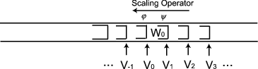
Multiresolution. \( { L^{2}(\mathbb{R}^{d}) } \)‑version (continuous); \( { \varphi \in V_{0} } \), \( { \psi \in W_{0} } \)
Figure 2 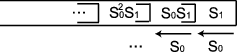
Multiresolution. \( { l^{2}(\mathbb{Z}) } \)‑version (discrete); \( { \varphi \in V_{0} } \), \( { \psi \in W_{0} } \)
The word “multiresolution” suggests a connection to optics from physics. So that should have been a hint to mathematicians to take a closer look at trends in signal and image processing!Moreover, even staying within mathematics, it turns out that as a general notion this same idea of a “multiresolution” has long roots in mathematics, even in such modern and pure areas as operator theory and Hilbert‐space geometry. Looking even closer at these interconnections, we can now recognize scales of subspaces (so‐called multiresolutions) in classical algorithmic construction of orthogonal bases in inner‐product spaces, now taught in lots of mathematics courses under the name of the Gram–Schmidt algorithm.Indeed, a closer look at good old Gram–Schmidt reveals that it is a matrix algorithm, Hence new mathematical tools involving non‐commutativity!
If the signal to be analyzed is an image, then why not select a fixed but suitable resolution (or a subspace of signals corresponding to a selected resolution), and then do the computations there? The selection of a fixed “resolution” is dictated by practical concerns. That idea was key in turning computation of wavelet coefficients into iterated matrix algorithms.As the matrix operations get large, the computation is carried out in a variety of paths arising from big matrix products.The dichotomy, continuous vs. discrete, is quite familiar to engineers. The industrial engineers typically work with huge volumes of numbers.
Numbers! – So why wavelets?Well, what matters to the industrial engineer is not really the wavelets, but the fact that special wavelet functions serve as an efficient way to encode large data sets – I mean encode for computations. And the wavelet algorithms are computational. They work on numbers. Encoding numbers into pictures, images, or graphs of functions comes later, perhaps at the very end of the computation. But without the graphics, I doubt that we would understand any of this half as well as we do now. The same can be said for the many issues that relate to the crucial mathematical concept of self‐similarity, as we know it from fractals, and more generally from recursive algorithms.


Bibliography
Aubert G, KornprobstP (2006) Mathematical problems in image processing. Springer, New York
Baggett L, JorgensenP, Merrill K, Packer J (2005) A non-MRA \( { C\sp r } \) frame wavelet withrapid decay. Acta Appl Math 1–3:251–270
Bratelli O, JorgensenP (2002) Wavelets through a looking glass: the world of the spectrum. Birkhäuser, Birkhäuser, Boston
Braverman M (2006)Parabolic julia sets are polynomial time computable. Nonlinearity19(6):1383–1401
Braverman M,Yampolsky M (2006) Non‐computable julia sets. J Amer Math Soc 19(3):551–578(electronic)
Bredies K, Lorenz DA,Maass P (2006) An optimal control problem in medical imageprocessing Springer, New York, pp 249–259
Daubechies I (1992)Ten lectures on wavelets. CBMS-NSF Regional Conference Series in Applied Mathematics,vol 61, SIAM, Philadelphia
Daubechies I (1993)Wavelet transforms and orthonormal wavelet bases. Proc Sympos Appl Math, Amer Math Soc 47:1–33, Providence
Daubechies I,Lagarias JC (1992) Two-scale difference equations. II. Local regularity, infinite productsof matrices and fractals. SIAM J Math Anal 23(4):1031–1079
Devaney RL, Look DM(2006) A criterion for sierpinski curve julia sets.Topology Proc30(1):163–179. Spring Topology and Dynamical SystemsConference
Devaney RL, RochaMM, Siegmund S (2007) Rational maps with generalized sierpinski gasket julia sets. Topol Appl154(1):11–27
Dutkay DE (2004)The spectrum of the wavelet galerkin operator. Integral Equations Operator Theory 4:477–487
Dutkay DE,Jorgensen PET (2005) Wavelet constructions in non‐linear dynamics.Electron Res AnnouncAmer Math Soc 11:21–33
Dutkay DE,Jorgensen PET (2006) Hilbert spaces built on a similarity and on dynamicalrenormalization. J Math Phys 47(5):20
Dutkay DE,Jorgensen PET (2006) Iterated function systems, ruelle operators, and invariant projectivemeasures. Math Comp 75(256):1931–1970
Dutkay DE,Jorgensen PET (2006) Wavelets on fractals. Rev Mat Iberoam 22(1):131–180
Dutkay DE, RoyslandK (2007) The algebra of harmonic functions for a matrix‐valued transferoperator. arXiv:math/0611539
Dutkay DE, RoyslandK (2007) Covariant representations for matrix‐valued transferoperators. arXiv:math/0701453
Heil C, Walnut DF(eds) (2006) Fundamental papers in wavelet theory. Princeton University Press, Princeton,NJ
Jorgensen PET(2003) Matrix factorizations, algorithms, wavelets. Notices Amer Math Soc 50(8):880–894
Jorgensen PET(2006) Analysis and probability: wavelets, signals, fractals. grad texts math,vol 234. Springer, New York
Jorgensen PET(2006) Certain representations of the cuntz relations, and a question on waveletsdecompositions. In: Operator theory, operator algebras, and applications. Contemp Math 414:165–188 Amer Math Soc, Providence
Liu F (2006)Diffusion filtering in image processing based on wavelet transform. Sci China Ser F 49(4):494–503
Milnor J (2004)Pasting together julia sets: a worked out example of mating.Exp Math13(1):55–92
Petersen CL, ZakeriS (2004) On the julia set of a typical quadratic polynomial with a siegel disk. AnnMath (2) 159(1):1–52
Skodras A,Christopoulos C, Ebrahimi T (2001) JPEG 2000 still image compression standard. IEEE SignalProcess Mag 18:36–58
Song MS (2006)Wavelet image compression. Ph.D. thesis, University of Iowa
Song MS (2006)Wavelet image compression. In: Operator theory, operator algebras, andapplications. Contemp. Math., vol 414. Amer. Math.Soc., Providence, RI, pp41–73
Strang G (1997)Wavelets from filter banks. Springer, Singapore, pp 59–110
Strang G (2000)Signal processing for everyone. Computional mathematics driven by industrial problems (Martina F 1999), pp 365–412. Lect Notes Math, vol 1739. Springer, Berlin
Strang G, Nguyen T(1996) Wavelets and filter banks. Wellesley-Cambridge Press, Wellesley
Usevitch BE(Sept. 2001) A tutorial on modern lossy wavelet image compression: foundations of jpeg2000. IEEE Signal Process Mag 18:22–35
Walker JS (1999)A primer on wavelets and their scientific applications. Chapman & Hall,CRC
Acknowledgments
We thank Professors Dorin Dutkay and Judy Packer for helpfuldiscussions.
Work supported in part by the U.S. National Science Foundation.
Author information
Authors and Affiliations
Editor information
Editors and Affiliations
Rights and permissions
Copyright information
© 2012 Springer-Verlag
About this entry
Cite this entry
Jorgensen, P.E.T., Song, MS. (2012). Comparison of Discrete and Continuous Wavelet Transforms. In: Meyers, R. (eds) Computational Complexity. Springer, New York, NY. https://doi.org/10.1007/978-1-4614-1800-9_34
Download citation
DOI: https://doi.org/10.1007/978-1-4614-1800-9_34
Publisher Name: Springer, New York, NY
Print ISBN: 978-1-4614-1799-6
Online ISBN: 978-1-4614-1800-9
eBook Packages: Computer ScienceReference Module Computer Science and Engineering