Analysis of Receptor–Ligand Interactions by Surface Plasmon Resonance

Abstract

Many immunological responses are often regulated by cell surface receptors in cell–cell recognition events. Such immune receptors on the cell surface typically exhibit low-affinity and fast-kinetic ligand interactions (e.g., K _d in the μM range, k _off  =  10⁻² to 20 s⁻¹). Real-time surface plasmon resonance (SPR) detection systems are generally useful for determining these binding parameters. However, several technical points should be considered because the determination of low-affinity binding and fast kinetics is often rather difficult. Here, we introduce a general procedure for SPR experiments and, moreover, show typical examples for ligand binding of immune cell surface receptors, including experimentally useful tips. We also show how to determine the thermodynamic characteristics using the nonlinear van’t Hoff and Arrhenius analyses. These affinity, kinetic, and thermodynamic parameters of immune–receptor binding are important for understanding immunological events as well as developing drugs and vaccines.

1 Introduction

Surface plasmon resonance (SPR) technology measures the mass concentration of biomolecules on sensor chips. Among the several SPR-based systems, the BIAcore (GE Healthcare) series are the most popular systems for monitoring the association and dissociation between ligands immobilized on the sensor chip and analytes flowed over the ligands in real time. The Biacore is useful for analyses with various nonlabeled biomolecules: proteins, peptides, nucleotides, carbohydrates, lipids, cells, viruses, etc. These biomolecules should be immobilized on appropriate sensor chips. If the regeneration step is optimized, then a sensor chip can be used more than 100 times. However, many immune cell surface receptors show low-affinity ligand binding with a fast dissociation rate, and thus do not require the regeneration step.

In order to understand receptor–ligand interactions, SPR is valuable because it can provide information not only about the specificity and affinity of binding, but also kinetic and thermodynamic information by monitoring in real time. This information is valuable for drug discovery and development.

Thermodynamic investigations of the quality of antibodies used for medical treatments are often required for the Food and Drug Administration (FDA) approval. The recent trend has promoted an easy and simple strategy for determining such parameters by using linear and nonlinear van’t Hoff analyses, which simply require the acquisition of affinity parameters at several different temperatures to determine the enthalpy, entropy, and heat capacity of ligand binding. While previous reports pointed out some discrepancy between the van’t Hoff and calorimetric analyses, the feasibility of the van’t Hoff analysis was ensured by recently accumulated evidence showing that these thermodynamic values are essentially in good agreement with those directly determined by isothermal titration calorimetry (ITC). Therefore, many researchers use SPR analysis to determine the thermodynamic parameters, and actually the most advanced T-100 model of the BIAcore system has an automatic routine procedure for determining the affinities at different temperatures and calculating the thermodynamic parameters using van’t Hoff analyses.

2 Materials

Several types of SPR equipment are available, including BIAcore (GE Healthcare), ProteOn XPR36 Technology (Bio-Rad Laboratories), and MultiSPRinter (Toyobo Corp.). While the latter two systems are generally more suitable for high-throughput measurements, the BIAcore is the most popular laboratory-based system. Therefore, here we mainly focus on the BIAcore system. The materials for SPR analyses using BIAcore systems are available from GE Healthcare.

2.1 Instruments

• 1. BIACORE instrument system

  GE Healthcare provides multiple systems according to the study design (e.g., basic research, drug discovery, manufacturing, and quality control) (http://www.biacore.com). See Table 1.

  Table 1 Biacore systems (November 2009)

• 2. Controlling PC.

• 3. BIACORE Control Software.

• 4. BIAevaluation Software.

• 5. Microcentrifuge.

2.2 Ligand Immobilization

Among the coupling methods, amine coupling is commonly used. GE Healthcare provides several other coupling kits: Thiol Coupling Kit, GST Kit for Fusion Capture, Mouse Antibody Capture Kit, and Human Antibody Capture Kit.

2.2.1 Amine Coupling: Immobilization of Amine Groups (Lysine and Unblocked N-Termini)

• 1. Sensor Chip CM5.

• 2. 100 mM N-hydroxysuccinimide (NHS) (see footnote 1).

• 3. 400 mM N-ethyl-N′-(3-dimethylaminopropyl) carbodiimide hydrochloride (EDC) (see footnote 1).

• 4. 1 M Ethanolamine hydrochloride (pH 8.5) (see footnote 1).

• 5. Ligand protein diluted by appropriate acetate buffer.

2.2.2 Intrinsic Ligand Thiol Coupling: Immobilization of a ligand possessing a surface-exposed free cysteine or disulfide

Ligands need to be reduced under nondenaturing conditions to generate the free cysteine.

• 1. Sensor Chip CM5.

• 2. 100 mM NHS (see footnote 2).

• 3. 400 mM EDC (see footnote 2).

• 4. 1 M Ethanolamine hydrochloride (pH 8.5) (see footnote 2).

• 5. 120 mM 2-(2-Pyridinyldithio)-ethaneamine hydrochloride (PDEA) (see footnote 2).

• 6. 150 mM Sodium borate buffer (pH 8.5) (see footnote 2).

• 7. 50 mM l-Cysteine (see footnote 2).

• 8. Ligand protein diluted by appropriate acetate buffer.

2.2.3 Surface Thiol Coupling: Immobilization of Amine or Carboxyl Groups

Reactive disulfides need to be introduced using PDEA.

• 1. Sensor Chip CM5.

• 2. 100 mM NHS (see footnote 2).

• 3. 400 mM EDC (see footnote 2).

• 4. 1 M Ethanolamine hydrochloride (pH 8.5) (see footnote 2).

• 5. 120 mM PDEA (see footnote 2).

• 6. 100 mM MES pH 5.0 (see footnote 2).

• 7. 40 mM Cystamine dihydrochloride (see footnote 2).

• 8. 150 mM Sodium borate buffer (pH 8.5) (see footnote 2).

• 9. 100 mM dithioerythritol (DTE) (see footnote 2).

• 10. 50 mM l-Cysteine (see footnote 2).

• 11. 1 M Sodium chloride (pH 4.0) (see footnote 2).

• 12. Ligand protein diluted by appropriate acetate buffer.

2.2.4 Aldehyde Coupling: Immobilization of Aldehyde Groups

Aldehydes need to be created by oxidizing cis-diols with periodate.

• 1. Sensor Chip CM5.

• 2. 100 mM NHS (see footnote 1).

• 3. 400 mM EDC (see footnote 1).

• 4. 1 M Ethanolamine hydrochloride (pH 8.5) (see footnote 1).

• 5. 5 mM Hydrazine monohydrate or 5 mM carbohydrazide.

• 6. 100 mM Sodium cyanoborohydride.

• 7. 100 mM Sodium acetate (pH 4.0, 5.5).

• 8. Sodium metaperiodate.

2.3 Running Buffers

The following buffers available from GE Healthcare are sterile-filtered and degassed, and thus are recommended as running buffers. Other buffers should be degassed and filtered through a 0.22-μm filter to remove particles. The buffers should include 0.005% Surfactant P20 to minimize the nonspecific adsorption of proteins.

• 1. HBS-EP: 0.01 M HEPES pH 7.4, 0.15 M NaCl, 3 mM EDTA, 0.005% Surfactant P20.

• 2. HBS-P: 0.01 M HEPES pH 7.4, 0.15 M NaCl, 0.005% Surfactant P20.

• 3. HBS-N: 0.01 M HEPES pH 7.4, 0.15 M NaCl.

2.4 Regeneration Buffers

See Table 2 for some commonly used regeneration buffers.

Table 2 Some commonly used regeneration buffers

3 Methods

3.1 Preparing the System

• 1. Turn on the Biacore system and the personal computer.

• 2. Start the Biacore Control Software.

• 3. Set the temperature (4–40°C for Biacore 2000, 3000, X100, and A100, and 4–45°C for Biacore T100). A temperature change of 5°C takes about 60 min. Since small air bubbles are often formed at >30°C, complete degassing of the running buffer is important. Biacore models X100, A100, T100, and Flexchip have an in-line degasser.

• 4. Prepare an appropriate running buffer.

• 5. Dock the appropriate sensor chip (see Table 3). The carboxymethylated dextran matrix is useful for:

  Table 3 Sensor Chips

  • (a) Making a hydrophilic environment on the surface of the sensor chip.

  • (b) Dramatically reducing nonspecific binding of samples.

  • (c) Increasing the flexibility of the immobilized ligands as if they were in solution.

  • (d) Easily immobilizing multiple ligands to create a three-dimensional structure on the chip.

• 6. Run Prime to equilibrate the flow system with running buffer. Place the running buffer and waste bottle at the appropriate locations before priming.

• 7. Set the Rack. Specialized racks and vials for each Biacore machine are available.

• 8. Check the condition of the Sensor Chip. View the dips by selecting View Dips. A normal dip shows a symmetric curve with sufficient depth (Fig. 1). On the other hand, an abnormal dip shows a shallow or jagged curve.

  Fig. 1.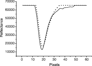

  

  Analysis of dips. Both the solid and dotted lines show normal dips.

3.2 Ligand Immobilization (Amine Coupling)

The molecules that are immobilized on the sensor chip are referred to as “Ligands.” Ligand immobilization is performed by direct covalent coupling or indirect capture coupling. The direct coupling methods can be used for almost fully purified proteins, but have some disadvantages: (1) heterogeneity of immobilized ligands and (2) inactivation of immobilized ligands due to blocking of the binding region by immobilization. On the other hand, the indirect coupling can be used only when a suitable binding site or a tag is available for the immobilized molecule. However, it has some advantages as compared to direct coupling: (1) inactivation of ligands does not normally happen, (2) a crude sample can be used, and (3) the orientation of the immobilized ligand is homogeneous. Particularly for receptors, this immobilization can replicate the cell surface orientation.

Among the coupling methods, a commonly used method is amine coupling, which we discuss here (Fig. 2). At first, carboxymethyl groups are activated by NHS, and highly reactive succinimide esters reacting with amines are created. Following the coupling of ligands, a high concentration of ethanolamine blocks the remaining activated carboxymethyl groups. References for other coupling methods are available in Biacore manuals or at the Web site (http://www.biacore.com).

Fig. 2.

Diagram of amine coupling method.

There are several Inject methods in the Control Software, and it is important to check the sample consumption volume to be prepared.

• (a) INJECT: Generally used inject method, Injected volume  +  30 μl necessary.

• (b) QUICKINJECT: Low sample consumption method, Injected volume  +  10 μl necessary. We usually use this Inject method, except for kinetic analysis.

• (c) KINJECT: Appropriate for kinetic analysis because of the low dispersion for samples sensitive to dilution with running buffer. Control the dissociation time after the sample is injected. Injected volume  +  40 μl necessary.

COINJECT (sequential injections of different samples), BIGINJECT (Large volume injection), and MANUAL INJECT are also available if necessary.

• 1. Run the sensorgram (10 μl/min) and wait until the baseline becomes stable. If the baseline is difficult to stabilize, increase the flow rate for a while.

• 2. Perform preconcentration to concentrate the ligand on the dextran matrix of the sensor chip by electrostatic attraction. Inject a small amount of ligand diluted with preconcentration buffer (acetate buffers at pH 4.0–5.5 are available from GE Healthcare) on the nonactivated sensor chip, and select an appropriate pH at which the ligands will become well-concentrated on the chip. In the case shown in Fig. 3, the ligand is most concentrated at pH 4.5. Generally, the highest pH that shows a sufficient response of immobilization should be normally selected for protein stability (see Note 1).

  Fig. 3.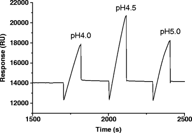

  

  Sensorgram of preconcentration of a ligand protein.

• 3. Mix the NHS and EDC in a 1:1 ratio gently (if necessary, degas by centrifugation), and immediately inject 100 μl of the mixture to activate the surface of the CM5 chip (10 μl/min). The next coupling step should be performed as soon as possible because the activated NHS–esters easily break down.

• 4. Inject the ligands (5–10 μl/min) diluted into the preconcentration buffer until the immobilization level reaches the target value. At least one flow cell should be used for a control ligand to record the nonspecific background response.

• 5. Inject 100 μl of ethanolamine hydrochloride (10 μl/min) to block the excess reactive surface.

• 6. Wash the chip with regeneration buffer (e.g., 10 mM glycine–HCl pH 2.0) if the proper regeneration method has already been determined. The regeneration step is useful to reuse the chip surface, but carefully confirm whether the ligand activity is unchanged and how many times regeneration can be performed. Ideally, regeneration should fulfill the following conditions: (1) maintaining the ligand activity, (2) completely dissociating the analytes, and (3) retaining the ligands on the sensor chip. In the case of typical fast ligand binding of immune cell surface receptors, such as MHC class I-LILRs (k _off  =  2.1  −  5.0 s⁻¹) (Table 4), the dissociation is quite fast and the sensorgram quickly returns to the baseline. In such cases, the regeneration step is not necessary. Some commonly used regeneration buffers are listed in Table 2.

  Table 4 Examples of kinetic parameters of receptor–ligand interactions

When we analyze receptor–ligand interactions by SPR, we generally use biotinylated recombinant proteins as ligands to achieve a homogeneous molecular orientation on the chip surface and to avoid blocking the binding sites by coupling. The biotinylated ligands are immobilized onto the Sensor Chip SA or the SA-coupled CM5 Chip.

For this method, we usually prepare the ectodomain of the ligand protein with the biotin ligase (birA) recognition sequence (GSLHHILDAQKMVWNHR) at the C-terminal end (for type I membrane proteins). Purified proteins with the birA recognition sequence are biotinylated by mixing the substrate samples, Biomix-A, and Biomix-B (8:1:1, respectively), and adding 1.0 μg of the birA enzyme (AVIDITY, LLC). Typically, for every 10 nmol of substrate at 40 μM, 2.5 μg of birA enzyme is recommended to complete the biotinylation in 30–40 min at 30°C. The biotinylated proteins are isolated from the free biotin by gel filtration chromatography or by dialysis. The purified biotinylated ligands are immobilized onto the SA-coupled CM5 chips. The amount of ligands needed for immobilization is modest (5–10 μg).

3.3 Preparing Analyte Samples

• 1. Purified analyte samples should be completely buffer-exchanged into the running buffer. If this step is not accomplished, a bulk effect obscuring rapid binding events could occur (see Note 2). The concentration of analyte protein is dependent on the K _d value, and the required volume is dependent on the analysis method.

• 2. Before injection, analyte samples should be degassed by centrifugation at room temperature.

3.4 Analysis of Protein Interactions

3.4.1 Equilibrium-Binding Analysis

An equilibrium-binding analysis is performed by multiple sequential injections of an analyte at different concentrations. The typical receptor–ligand interaction is quite weak (K _d in the μM range) and shows fast association and dissociation (Table 4). In this case, the K _d value can be measured directly by an equilibrium-binding analysis. Here, we describe LILRB2 (22 kDa)–HLA-G (45 kDa) binding as an example. As for high-affinity interactions, an equilibrium-binding analysis is not suitable due to the very slow dissociation rates. Furthermore, if the binding is very strong and the bound analyte is difficult to dissociate from the ligands, then a regeneration step should be included after the injection step.

3.4.1.1 Experiment

• 1. Dock a new CM5 chip, equilibrate the chip by running Prime with HBS–EP buffer, and immobilize SA diluted with 10 mM sodium acetate pH 5.0 buffer by amine coupling (>10,000 RU) (see Note 3).

• 2. Immobilize the ligands, including biotinylated BSA as a control protein on SA-immobilized Fc1 (2,000 RU) and C-terminal biotinylated HLA-G on SA-immobilized Fc2 (2,000 RU). Biotinylated HLA-G is prepared by a refolding method and purified as described previously (1, 2). Since the Biacore 3000 system has four flow cells, up to three kinds of ligands can be immobilized, in addition to a control ligand.

• 3. Prepare the analyte LILRB2 protein by the refolding method (3). Purified LILRB2, concentrated to 36.6 μM in HBS–EP buffer, is serially diluted twofold with HBS–EP buffer (0.07–36.6 μM). Centrifuge all samples at max speed (e.g., 16,000 × g) in a microcentrifuge for 5 min at RT. The sample concentration needs to be sufficiently higher than the expected K _d. If there is no information available about the K _d, then about 50 μM will be sufficient to calculate the K _d of most of immune receptor–ligand interactions.

• 4. Inject 5 μl of the analyte in flow cells Fc1–Fc2 sequentially (10 μl/min) by Quickinject, from low to high concentration samples. Since the binding affinity between HLA-G and LILRB2 is weak and displays fast association/dissociation, it can be considered that there is no difference in the concentration in each flow cell. The time to the next injection should be estimated from the k _off.

3.4.1.2 Data Analysis

Raw data from an equilibrium-binding analysis are shown in Fig. 4. Usually, we use a program to record the response (RU) 10 s before injection as a Baseline and 20 s after injection as a Response.

Fig. 4.

Sensorgram of equilibrium-binding analysis. The gray line is BSA (Fc1), and the black line is LILRB2 (Fc2). Ten serially diluted LILRB2 samples are injected from low to high concentrations.

• 1. For each serially diluted analyte sample, the actual binding response is calculated from [Response]–[Baseline].

• 2. The binding response (RU) at each concentration is calculated by subtracting the response measured in the control flow cell (Fc1: BSA) from the response in the sample flow cell (Fc2: HLA-G). This value is applied to the simple 1:1 Langmuir-binding model (A  +  B  «  AB). The Langmuir model is the most commonly used model to calculate binding affinity. This model is applied to the simple situation of an interaction between two samples (A, B). It is hypothesized that both the analyte and ligand are homogeneous, and that the analyte is monovalent.

• 3. Plot the analyte concentration on the X-axis and the Response (RU) on the Y-axis, as shown in Fig. 5. Affinity constants (K _d) are derived by nonlinear curve fitting of the standard Langmuir-binding isotherm:

  $$y={R}_{\mathrm{max}} \cdot \text x/\left({K}_{\text{d}}+x\right) {R}_{\mathrm{max}} :\rm{ maximum \ response \ units}.$$

  Fig. 5.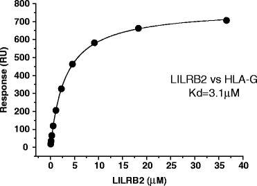

  

  The affinity of the LILRB2–HLA-G interaction. The responses are plotted against the concentrations of injected LILRB2 protein. The solid line represents direct nonlinear fit of the 1:1 Langmuir-binding isoform to the data. The K _d value is determined as 3.1 μM.

• 4. The affinity constant (K _d) is also derived by Scatchard analysis, as shown in Fig. 6.

  Fig. 6.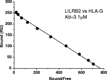

  

  The Scatchard plot of the LILRB2–HLA-G interaction. The solid line is the linear fit. The K _d value is determined as 3.1 μM.

3.4.2 Kinetic Analysis

SPR analysis is also used to analyze high-resolution kinetic parameters. From a sensorgram, such as that in Fig. 7, kinetic parameters (k _a, k _d) are calculated. Here, we describe LILRB1 (22 kDa)–HLA-G (45 kDa) binding as an example. If the binding is quite strong and the bound analyte is difficult to dissociate from the ligands, then the regeneration step should be added after the injection, as shown in Fig. 7. From the association phase, the association rate constant (k _a, M/s) between the ligand and the analyte is calculated, and the dissociation rate constant (k _d, 1/s) is calculated from the dissociation phase.

Fig. 7.

Typical sensorgram of a binding analysis. During the association phase, the ligand binding is reflected by an increasing Response. At the end point of the analyte injection, the running buffer is flowed over the ligand and the dissociation phase begins. In order to start the new cycle of injection, the Response should return to the baseline level. In this case, the ligand is regenerated by the injection of regeneration buffer.

To avoid mass transport limitations and rebinding of analytes to the immobilized ligand before leaving the sensor surface, an excess of ligands should not be immobilized (see Note 4). In the beginning, multiple immobilization levels of ligand should be assessed. GE Healthcare recommends the level of immobilization as described below (s means the number of ligand-binding sites):

$$\text{Min }\left(\text{RU}\right) =200\times 1/s\times \left(\text{Ligand \ Mw}\text{}/ \text{Analyte \ Mw}\right)$$

$$\begin{array}{ll}\text{Max }\left(\text{RU}\right) = & 1,000\times 1/s\times \left(\text{Ligand \ Mw} / \text{Analyte \ Mw}\right)\\ {}&\text{Mw}:\text{ molecular \ weight}.\end{array}$$

In the case of LILRB1 (22,000 Da) and HLA-G (45,000 Da),

$$ \text{Min }\left(\text{RU}\right) = 200\times 1/1\times \left(45,000/22,000\right)=409 \ \text{RU}$$

$$ \text{Max }\left(\text{RU}\right)=1,000\times 1/1\times \left(45,000/22,000\right)=2,045 \ \text{ RU}.$$

3.4.2.1 Experiment

• 1. Dock the CM5 chip, equilibrate the chip by running Prime with HBS–EP buffer, and immobilize SA diluted with 10 mM sodium acetate pH 5.0 buffer by amine coupling (>10,000 RU).

• 2. Immobilize the ligands, biotinylated BSA as a control protein on SA-immobilized Fc1 (800 RU) and biotinylated HLA-G on SA-immobilized Fc2 (800 RU). If it is possible, immobilize the ligand at different levels using three flow cells (Fc2–Fc4).

• 3. Prepare the analyte LILRB1 protein by the refolding method (3). Purified LILRB1 was concentrated to 3.0 μM in HBS–EP buffer and serially diluted twofold with HBS–EP buffer (0.19–3.0 μM). Centrifuge all samples at max speed (e.g., 16,000×g) in a microcentrifuge for 5 min at RT. In the kinetic analysis, Kinject (Injected volume  +  40 μl) should be used in order to avoid sample dilution with running buffer. Furthermore, the analyte sample should be flowed over each flow cell independently, not sequentially, because the highest resolution detection is suitable for fast kinetics (see the following paragraph).

• 4. Inject 5 μl of the analyte in flow cells Fc1–Fc2 sequentially (50 μl/min) by Kinject, from low to high concentration ­samples. A higher flow rate should be used than that for an equilibrium-binding analysis in order to minimize mass transport effects. Data collection at the maximum resolution (Data collection rate  =  high (see footnote ¹)) and only one flow cell detection mode are recommended for measurements of very fast kinetics, such as cell surface receptor–ligand interactions. The durations of the association and dissociation phases should be determined in a preliminary experiment.

3.4.2.2 Data Analysis (BIAevaluation Software)

Generally, the association of Analyte A and Ligand B results in the formation of complex AB.

$$\text{A}+\text{B }\underset{{k}_{d}}{\overset{{k}_{a}}{\rightleftarrows }}\text{ AB},$$

where k _a is association rate constant (M⁻¹/s) and

k _d is dissociation rate constant (1/s).

When the response achieves equilibrium, the rate of the concentration changes, which is dependent on the concentrations of A, B, and AB, and becomes zero.

$$\text{d}\left[\text{AB}\right]/\text{d}t={k}_{\text{a}}\left[\text{A}\right]\left[\text{B}\right]-{k}_{\text{d}}\left[\text{AB}\right]$$

(1)

$$ {k_{\text{d}}}/{k_{\text{a}}} = { }\left[ {\text{A}} \right]\left[ {\text{B}} \right]/\left[ {\text{AB}} \right]{ } = {K_{\text{d}}}{ }\left( {{\text{dissociation constant}},{\text{ M}}} \right), $$

K _a (association constant, 1/M)  =  1/K _d.

A smaller K _d means higher affinity.

In the Biacore systems, Analyte A always flows over Ligand B at the same concentration. Therefore, [A]  =  [A]₀, [B]  =  [B]₀  −  [AB].

$$ \text{d}\left[\text{AB}\right]/\text{d}t={k}_{\text{a}}\left[\text{A}\right]\left[\text{B}\right]-{k}_{\text{d}}\left[\text{AB}\right]={k}_{\text{a}}\left[\text{A}\right]{\text{}}_{0}\left(\left[\text{B}\right]{\text{}}_{0}-\left[\text{AB}\right]\right)-{k}_{\text{d}}\left[\text{AB}\right].$$

Next, relate the parameters in Eq. (1) to the SPR parameters. The concentration of complex AB ([AB]) is the response R (RU), [B]₀ is the maximum response R _max (RU), and the concentration of Analyte A [A]₀ is C.

$$\begin{array}{l}\text{d}R/\text{d}t={k}_{\text{a}}C\left({R}_{\mathrm{max}}-R\right)-{k}_{\text{d}}R\\ \quad \quad \quad={k}_{\text{a}}C{R}_{\mathrm{max}}-\left({k}_{\text{a}}C+{k}_{\text{d}}\right)R\\ \left({k}_{\text{a}}C+{k}_{\text{d}}\right):\text{pseudo \ reaction \ rate \ constant}\text{.}\end{array}$$

(2)

The change rate of R follows a pseudo-first-order reaction. Here, the calculated pseudo (k _a C  +  k _d) is dependent on C; therefore, the k _a can be calculated by plotting (k _aC  +  k _d) against the known C. By using the BIA evaluation software supplied by GE Healthcare, nonlinear fitting of the sensorgram by a nonlinear least-squares analysis can be performed, as described below.

• 1. Start the BIAevaluation software.

• 2. Open the result file, and display the sensorgram curves of the same analyte concentration of control (BSA) and HLA-G (Fc1 and Fc2, respectively).

• 3. Subtract the response in the control flow cell (Fc1: BSA) from the response in the sample flow cell (Fc2: HLA-G). It is important to adjust the baseline (Y-axis) just before the injection point and injection/dissociation point (X-axis) before subtracting. The subtraction of the control response from the sample response is performed for each analyte concentration response curve (Fig. 8).

  Fig. 8.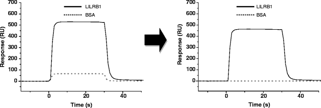

  

  Sensorgram of a kinetic analysis between HLA-G and LILRB1 at a single concentration. The solid line is the sensorgram of LILRB1, and the dotted line is the sensorgram of BSA after adjustment of the X- and Y-axes. Sensorgrams before subtraction of the control (left  ) and after subtraction (right  ) are shown.

• 4. Display the response plot drawn by (Fc2–Fc1) all dilution series samples (0.19, 0.38, 0.75, 1.5, and 3.0 μM of LILRB1).

• 5. Perform the fitting using the appropriate fitting model. In the case of the LILRB1–HLA-G interaction, the global fitting analysis using a 1:1 Langmuir-binding model was simultaneously performed with the raw data for the association and dissociation phases at different concentrations of LILRB1 (Fig. 9). As shown in Fig. 9, the small variation in the residuals (see footnote 4) means that the model is suitable for this analysis.

  Fig. 9.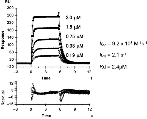

  

  The global fitting kinetic analyses of LILRB1 against HLA-G (4). The square dots are actual sensorgram data and the solid lines are nonlinear fits. The lower panel shows the residual errors from the fits. Kinetic parameters are also shown.

Several simultaneous k _a/k _d fitting models are available in the BIAevaluation software.

• (a) 1:1 Langmuir-binding model: Interaction between ligand A and analyte B. The simplest model, which is equivalent to the Langmuir isotherm for adsorption to a surface.

  $$ \text{A }+\text{ B }\leftrightarrow \text{ AB}$$

• (b) 1:1 binding with drifting baseline: Sensorgram showing a linearly drifting baseline. Before using this model, try to eliminate the drift by subtracting the control sensorgram.

  $$ \text{A }+\text{ B }\leftrightarrow \text{ AB}$$

• (c) 1:1 binding with mass transfer: Interaction showing mass transfer limitations. Before using this model, try to increase the flow rate or immobilize ligands at a lower level.

  $$ \text{A }+\text{ B }\leftrightarrow \text{ AB}$$

• (d) Bivalent analyte: Interaction of a bivalent or dimeric analyte.

  $$ \text{A }+\text{ B }\leftrightarrow \text{ AB}$$
  $$ \text{AB }+\text{ B }\leftrightarrow {\text{ AB}}_{2}$$

• (e) Heterogeneous analyte–competition reactions: Two kinds of analytes competitively interact with the ligand.

  $$ {\text{A}}_{1}+\text{ B }\leftrightarrow {\text{A}}_{1}\text{B}$$
  $$ {\text{A}}_{2}+\text{ B }\leftrightarrow {\text{A}}_{2}\text{B}$$

• (f) Heterogeneous ligand–parallel reaction: Interactions between an analyte and a ligand possessing two binding sites with different binding affinities.

  $$ \text{A }+{\text{B}}_{1}\leftrightarrow {\text{ AB}}_{1}$$
  $$ \text{A }+{\text{B}}_{2}\leftrightarrow {\text{ AB}}_{2}$$

• (g) Two-state reactions (conformation change): After formation of the AB complex, the complex changes its conformation.

  $$ \text{A }+\text{ B }\leftrightarrow \text{ AB }\leftrightarrow {\text{ AB}}^{\text{x}}$$

Additionally, separate k _a/k _d models that fit k _a and k _d separately and describe only the association or dissociation phase of the sensorgram can be generated by the BIAevaluation software. However, simultaneous k _a/k _d fitting is preferable, if possible.

3.4.3 Thermodynamic Analysis

The Biacore system can strictly control the temperature of flow cells. By measuring the change in the binding affinity at different temperatures, it is possible to estimate the thermodynamic parameters using van’t Hoff analysis, as described below. Here, we describe LILRB1 (22 kDa)–HLA-G (45 kDa) binding as an example.

3.4.3.1 Experiment

• 1. Dock the CM5 chip, equilibrate the chip by running Prime with HBS–EP buffer, and immobilize SA (10 mM sodium acetate pH 5.0 buffer) by amine coupling (>10,000 RU).

• 2. Immobilize the ligands: Biotinylated BSA as a control protein on SA-immobilized Fc1 (2,000 RU) and C-terminal biotinylated HLA-G on SA-immobilized Fc2 (2,000 RU).

• 3. Set the temperature (e.g., 10°C, 15°C, 20°C, 25°C, and 30°C) and wait until the measured temperature is stable.

• 4. Prepare the analyte LILRB1 protein (50 μM) in HBS–EP buffer and serially dilute it twofold with HBS–EP buffer (0.2–50 μM). Centrifuge all samples at max speed (e.g., 16,000×g) in a microcentrifuge for 5 min at RT.

• 5. Inject 5 μl of the analyte Fc1  →  Fc2 sequentially (10 μl/min) by Quickinject from low to high concentration samples.

3.4.3.2 Data Analysis

By measuring the change in the binding affinity at different temperatures, the van’t Hoff enthalpy can be calculated using the following equations.

The change of Gibbs energy are

$$ \Delta G/T=\Delta H/T-\Delta S$$

$$\text{d}\left(\Delta G/T\right)/\text{d}T=\text{d}\Delta H/T\text{d}T-\Delta H/{T}^{2}-\text{d}\Delta S/\text{d}T.$$

(3)

Here,

$$ \text{d}\Delta H=\Delta {C}_{\text{p}}\text{d}T\text{and }$$

$$ \text{d}\Delta H=\Delta {C}_{\text{p}}\text{d}T\text{and }$$

is applied to Eq. (3).

$$\begin{array}{c}\text{d}(\Delta G/T)/\text{d}T=\Delta {C}_{\text{p}}/T-\Delta H/{T}^{2}-\Delta {C}_{\text{p}}/T\\ =-\Delta H/{T}^{2}.\end{array}$$

(4)

The standard state Gibbs energy change upon binding was obtained from

$$ \Delta G=RT\mathrm{ln}{K}_{d},$$

where K _d is the dissociation constant and R is the gas constant. Therefore,

$$ \text{d}\mathrm{ln}{K}_{\text{d}}/\text{d}\left(1/T\right)=-\Delta H/R.$$

The enthalpy (ΔH) can be calculated by plotting ln K _d against 1/T.

On the other hand, the ΔG values of each data set are plotted against the temperatures, and are fitted with the nonlinear van’t Hoff equation ΔG  =  ΔH  −  TΔS  +  ΔC _p(T  −  298.15)  −  ΔC _p Tln(T/298.15), where ΔH and ΔS are the binding enthalpy and entropy at 298.15 K, respectively, and ΔC _p is the heat capacity, which is assumed to be temperature-independent.

• 1. The K _ds are determined at different temperatures by an equilibrium-binding analysis (see Subheading 3.4.1).

• 2. The Gibbs energy (ΔG) at each temperature point is obtained from the K _d.

$$ \Delta G=RT\mathrm{ln}{K}_{\text{d}}.$$

ΔG is plotted against the temperatures and is fitted with the nonlinear van’t Hoff equation (Fig. 10). ΔH, ΔS, and ΔC _p are obtained simultaneously from this fitting (Table 5). These data are in good agreement with the values obtained from an ITC analysis (ΔG  =  −7.0 kcal/mol, ΔH  =  2.4 kcal/mol, −TΔS  =  −9.4 kcal/mol, ΔC _p  =  −0.22 kcal/mol K) (4).

Fig. 10.

The plots of temperature dependence of ΔG (4). ΔG values at five temperature points were obtained from equilibrium-binding analyses. Filled triangles represent the plot fitted with the nonlinear van’t Hoff equation of the association between LILRB1 and HLA-G. Filled circles and squares are the associations with other tested HLA-class I molecules.

Table 5 Examples of the thermodynamic parameters of the receptor–ligand interactions

3.4.4 Activation Energy Analysis

Binding rate constants generally increase with temperature. The extent of this increase is a measure of the amount of thermal energy required to cross an energy barrier preventing the association or dissociation, and is referred to as the activation energy of association or dissociation (E ^on_a or E ^off_a ). By measuring the change in the kinetic parameters at different temperatures, the activation energies can be calculated. Here, we describe LILRB1 (22 kDa)–HLA-G (45 kDa) binding as an example.

3.4.4.1 Experiment

• 1. Dock the CM5 chip, equilibrate the chip by running Prime with HBS-EP buffer, and immobilize SA (10 mM sodium acetate pH 5.0 buffer) by amine coupling (>10,000 RU).

• 2. Immobilize the ligands: Biotinylated BSA as a control protein on SA-immobilized Fc1 (800 RU) and biotinylated HLA-G on SA-immobilized Fc2 (800 RU).

• 3. Set the temperature (e.g., 10°C, 15°C, 20°C, 25°C, and 30°C) and wait until the measured temperature is stable.

• 4. Prepare the analyte LILRB1 (3.0 μM) in HBS–EP buffer and serially dilute it twofold with HBS–EP buffer (0.19–3.0 μM). Centrifuge all samples at max speed (e.g., 16,000×g) in a microcentrifuge for 5 min at RT.

• 5. Inject 5 μl of the analyte Fc1  →  Fc2 sequentially (50 μl/min) by Kinject, from low to high concentration samples.

3.4.4.2 Data Analysis

The activation energy of association or dissociation (E ^on_a or E ^off_a ) was obtained using the Arrhenius equation. By assuming E _a is constant over the temperature range analyzed,

$$ \mathrm{ln}k=\mathrm{ln}A-{E}_{\text{a}}/RT,$$

where k is the k _on or k _off, A is a constant known as a preexponential factor, and R is the gas constant.

The reaction enthalpy can be calculated from the relationship,

$$ \Delta H={E}_{\text{a}}^{\text{on}}-{E}_{\text{a}}^{\text{off}}.$$

• 1. The k _a or k _d is determined at different temperatures by kinetic analysis (see Subheading 3.4.2).

• 2. E ^on_a and E ^off_a are obtained from Arrhenius plots (Fig. 11) (4). In the case of association between LILRB1 and HLA-G, the small temperature dependency resulted in low E ^on_a and E ^off_a values (E ^on_a  =  5.4 kcal/mol, E ^off_a  =  2.2 kcal/mol, ΔH  =  3.2 kcal/mol).

  Fig. 11.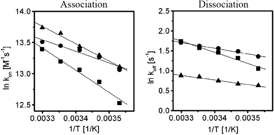

  

  Temperature dependencies of k _on (left  ) and k _off (right  ) (4). Arrhenius plots of the natural logarithm on and off rates for LILRB1 binding derived over a range of temperatures (10–30°C). Filled circles and squares are associations with other tested HLA-class I molecules.

3.4.5 Shutdown

The shutdown methods differ, according to how long the system will not be in use (see Note 5):

• (a) <3 days until the next experiment using the same sensor chip

  The Standby procedure is useful to keep the instrument with the used sensor chip filled with the running buffer. The Standby procedure keeps the Biacore running at a slow flow rate (5 μl/min) for max 96 h. Make sure that sufficient running buffer is available.

• (b) 3–5 days

  To shut down the system for up to 5 days, run Prime with water followed by run Close with water.

• (c) >5 days

  Run shutdown method with 70% ethanol.

4 Notes

• 1. Ligands that are difficult to preconcentrate (low-weight molecules and peptides) should be diluted with 10 mM borate buffer (pH 8.5) because the response between NHS and amine is most efficient at pH 8.5.

• 2. Bulk effect: Bulk effects are due to differences in the refractive indexes of the running buffer and the sample solution.

• 3. In Biacore systems, one RU represents the binding of about 1 pg/mm².

• 4. Mass transport limitation and rebinding: The situation in which a massive amount of ligand causes two important problems in the kinetic analysis by SPR. The first one is the mass transport limitation, in which the rate at which the analyte binds the ligand can exceed the rate at which it is delivered to the surface. The reaction rate is limited by the physical transport of the analyte. When k _on and k _off are faster than the diffusion rate of the analyte, the depletion of the analyte close to the matrix occurs during the association phase, and then the binding is controlled by diffusion and not by interaction. As a result, an apparent k _on is calculated that is slower than the actual k _on. The effect of the high flow rate on mass transfer is not very large. On the other hand, the density of the immobilized ligand is quite important. Minimizing the ligand density is the most effective way to reduce mass transfer limitations. The next potential problem is the rebinding of analytes to the ligand before they leave the sensor surface. Consequently, the apparent k _off is slower than the actual k _off. This can also be avoided by decreasing the level of immobilized ligands.

• 5. Storage of sensor chips: Used sensor chips can be stored under dry or wet (with buffer in a 50-mL tube) conditions. Stable protein-, peptide-, or DNA-immobilized sensor chips can be stored under dry conditions.

• 6. Single-cycle kinetics (23): As shown in Table 1, Biacore X100 and T100 are capable of performing single-cycle kinetics. Since single-cycle kinetics enables kinetic analysis without the regeneration of a sensor chip, analyte samples are injected one after the other in the same cycle. This method is suitable for molecular interactions for which the kinetic parameters were previously difficult to determine due to the inability to regenerate ligands. Furthermore, it reduces the time required to develop the assay conditions. The Biacore software recommends five sample concentrations and a duplication cycle for this analysis to ensure a robust evaluation.

References

Garboczi D.N., Hung D.T. and Wiley D.C. (1992) HLA-A2-peptide complexes: refolding and crystallization of molecules expressed in Escherichia coli and complexed with single antigenic peptides. Proc Natl Acad Sci USA, 89, 3429–3433.
Reid S.W., Smith K.J., Jakobsen B.K., O’Callaghan C.A., Reyburn H., Harlos K., et al. (1996) Production and crystallization of MHC class I B allele single peptide complexes. FEBS Lett, 383, 119–123.
Shiroishi M., Tsumoto K., Amano K., Shirakihara Y., Colonna M., Braud V.M., et al. (2003) Human inhibitory receptors Ig-like transcript 2 (ILT2) and ILT4 compete with CD8 for MHC class I binding and bind preferentially to HLA-G. Proc Natl Acad Sci USA, 100, 8856–8861.
Shiroishi M., Kuroki K., Tsumoto K., Yokota A., Sasaki T., Amano K., et al. (2006) Entropically driven MHC class I recognition by human inhibitory receptor leukocyte Ig-like receptor B1 (LILRB1/ILT2/CD85j). J Mol Biol, 355, 237–248.
Chapman T.L., Heikeman A.P. and Bjorkman P.J. (1999) The inhibitory receptor LIR-1 uses a common binding interaction to recognize class I MHC molecules and the viral homolog UL18. Immunity, 11, 603–613.
Maenaka K., Juji T., Nakayama T., Wyer J.R., Gao G.F., Maenaka T., et al. (1999) Killer cell immunoglobulin receptors and T cell receptors bind peptide-major histocompatibility complex class I with distinct thermodynamic and kinetic properties. J Biol Chem, 274, 28329–28334.
Wyer J.R., Willcox B.E., Gao G.F., Gerth U.C., Davis S.J., Bell J.I., et al. (1999) T cell receptor and coreceptor CD8 alpha bind peptide-MHC independently and with distinct kinetics. Immunity, 10, 219–225.
Tabata S., Kuroki K., Wang J., Kajikawa M., Shiratori I., Kohda D., et al. (2008) Biophysical characterization of O-glycosylated CD99 recognition by paired Ig-like type 2 receptors. J Biol Chem, 283, 8893–8901.
Bakker T.R., Piperi C., Davies E.A. and Merwe P.A. (2002) Comparison of CD22 binding to native CD45 and synthetic oligosaccharide. Eur J Immunol, 32, 1924–1932.
van der Merwe P.A., Bodian D.L., Daenke S., Linsley P. and Davis S.J. (1997) CD80 (B7-1) binds both CD28 and CTLA-4 with a low affinity and very fast kinetics. J Exp Med, 185, 393–403.
Maenaka K., van der Merwe P.A., Stuart D.I., Jones E.Y. and Sondermann P. (2001) The human low affinity Fcgamma receptors IIa, IIb, and III bind IgG with fast kinetics and distinct thermodynamic properties. J Biol Chem, 276, 44898–44904.
Willcox B.E., Gao G.F., Wyer J.R., Ladbury J.E., Bell J.I., Jakobsen B.K., et al. (1999) TCR binding to peptide-MHC stabilizes a flexible recognition interface. Immunity, 10, 357–365.
Ding Y.H., Baker B.M., Garboczi D.N., Biddison W.E. and Wiley D.C. (1999) Four A6-TCR/peptide/HLA-A2 structures that generate very different T cell signals are nearly identical. Immunity, 11, 45–56.
Wild M.K., Huang M.C., Schulze-Horsel U., van der Merwe P.A. and Vestweber D. (2001) Affinity, kinetics, and thermodynamics of E-selectin binding to E-selectin ligand-1. J Biol Chem, 276, 31602–31612.
Nicholson M.W., Barclay A.N., Singer M.S., Rosen S.D. and van der Merwe P.A. (1998) Affinity and kinetic analysis of L-selectin (CD62L) binding to glycosylation-dependent cell-adhesion molecule-1. J Biol Chem, 273, 763–770.
Mehta P., Cummings R.D. and McEver R.P. (1998) Affinity and kinetic analysis of P-selectin binding to P-selectin glycoprotein ligand-1. J Biol Chem, 273, 32506–32513.
O’Callaghan C.A., Cerwenka A., Willcox B.E., Lanier L.L. and Bjorkman P.J. (2001) Molecular competition for NKG2D: H60 and RAE1 compete unequally for NKG2D with dominance of H60. Immunity, 15, 201–211.
Boniface J.J., Reich Z., Lyons D.S. and Davis M.M. (1999) Thermodynamics of T cell receptor binding to peptide-MHC: evidence for a general mechanism of molecular scanning. Proc Natl Acad Sci USA, 96, 11446–11451.
Anikeeva N., Lebedeva T., Krogsgaard M., Tetin S.Y., Martinez-Hackert E., Kalams S.A., et al. (2003) Distinct molecular mechanisms account for the specificity of two different T-cell receptors. Biochemistry, 42, 4709–4716.
Garcia K.C., Radu C.G., Ho J., Ober R.J. and Ward E.S. (2001) Kinetics and thermodynamics of T cell receptor-autoantigen interactions in murine experimental autoimmune encephalomyelitis. Proc Natl Acad Sci USA, 98, 6818–6823.
Lee J.K., Stewart-Jones G., Dong T., Harlos K., Di Gleria K., Dorrell L., et al. (2004) T cell cross-reactivity and conformational changes during TCR engagement. J Exp Med, 200, 1455–1466.
Davis-Harrison R.L., Armstrong K.M. and Baker B.M. (2005) Two different T cell receptors use different thermodynamic strategies to recognize the same peptide/MHC ligand. J Mol Biol, 346, 533–550.
Karlsson R., Katsamba P.S., Nordin H., Pol E. and Myszka D.G. (2006) Analyzing a kinetic titration series using affinity biosensors. Anal Biochem, 349, 136–147.
Author information
Authors and Affiliations
Corresponding author
Editor information
Editors and Affiliations
Rights and permissions
Copyright information
© 2011 Springer Science+Business Media, LLC
About this protocol
Cite this protocol
Kuroki, K., Maenaka, K. (2011). Analysis of Receptor–Ligand Interactions by Surface Plasmon Resonance. In: Rast, J., Booth, J. (eds) Immune Receptors. Methods in Molecular Biology, vol 748. Humana Press, Totowa, NJ. https://doi.org/10.1007/978-1-61779-139-0_6
Download citation
DOI: https://doi.org/10.1007/978-1-61779-139-0_6
Published:
Publisher Name: Humana Press, Totowa, NJ
Print ISBN: 978-1-61779-138-3
Online ISBN: 978-1-61779-139-0
eBook Packages: Springer Protocols