Real-Time PCR to Identify Staphylococci and Assay for Virulence from Blood

Abstract

The genus Staphylococcus includes pathogenic and non-pathogenic facultative anaerobes. Due to the plethora of virulence factors encoded in its genome, the species Staphylococcus aureus is known to be the most pathogenic. S. aureus strains harboring genes encoding virulence and antibiotic resistance are of public health importance. In clinical samples, however, pathogenic S. aureus is often mixed with putatively less pathogenic coagulase-negative staphylococci (CoNS), both of which can harbor mecA, the genetic driver for staphylococcal methicillin-resistance. In this chapter, the detailed practical procedure for operating a real-time pentaplex PCR assay in blood cultures is described. The pentaplex real-time PCR assay simultaneously detects markers for the presence of bacteria (16S rRNA), coagulase-negative staphylococcus (cns), S. aureus (spa), Panton-Valentine leukocidin (pvl), and methicillin resistance (mecA).

1 Introduction

The genus Staphylococcus comprises facultative anaerobes, that is, they are capable of growth both aerobically and anaerobically. Staphylococci were historically delineated into two types; namely pathogenic and non-pathogenic. Both types of Staphylococcus spp. have been detected in healthy subjects in the community and in hospital patients [1, 2]. The staphylococci are relevant in public health because of their association with diverse infections including pneumonias, skin diseases, septicaemias, enteric infections, toxic shock syndromes, wound infections, bed sores, and urinary tract infections. The genomes of many staphylococci harbor genes encoding antibiotic resistance and horizontal genetic transfer (HGT) are well reported between different species; the mecA gene that codes for low-affinity penicillin-binding protein (PBP2a) is a typical example [3, 4]. S. aureus genomes are especially known for making a variable number of molecules associated with virulence and disease pathogenesis [5]. Some of the virulence proteins associated with S. aureus are encoded by species-specific genes such as spa (the gene that codes for staphylococcal proteinA, Spa), coa (the gene coding for coagulase, Coa), and nuc (the gene encoding staphylococcal thermonuclease, Nuc): these molecules have only been found in S. aureus, and not in the other staphylococci often called coagulase negative staphylococci (CoNS). Some S. aureus strains, however, harbor other virulence factors not commonly shared within the species; typical examples are the tst gene that codes for staphylococcal toxic shock toxin (Tst), the co-transcribed bi-component lukSF-PV (also called pvl) operon for the Panton-Valentine leukocidin toxin (PVL), and the enterotoxins that are very diverse. For this reason, it is important in diagnostic bacteriology to identify staphylococci and to assay for virulence, especially in blood. Although staphylococci have been identified by phenotypic methods over the years, which is still the current practice in some laboratories, the emergence of antibiotic resistance and virulence in many bacterial species including the staphylococci challenge the reliability of agar-based bacteriological tests [6, 7]. The way around this is that several laboratories have begun introducing diagnostic tests based on the polymerase chain reaction (PCR), including multiplexed assays that detect more than one DNA target in a PCR well [8, 9]. One of the off-shoots of conventional PCR is the application of florescent dyes to monitor amplification products as they accumulate. This is the basic principle of the modern real-time PCR that circumvents the need for resolution of PCR amplification products in gel electrophoresis. In this chapter, the steps toward the development and validation of a real-time PCR assay capable of detecting and quantifying five DNA targets for the identification of ubiquitous bacteria (16S rRNA), S. aureus (spa), the PVL operon (pvl), methicillin resistance (mecA), and marker for CoNS (cns) are described. By virtue of specificity (100%), sensitivity (Limit of detection, LoD = 1 colony forming unit per ml), simplicity, and accuracy, this method will be useful in clinical diagnostic settings.

2 Materials

2.1 Specialist Equipment

• 1. DNA work station: DNA work station is required for the preparation of DNA and solutions. L020—XL—GC (Kisker Biotech GmbH & Co. KG, Germany) is recommended (see Note 1 ).

• 2. Centrifuge for real-time PCR multiwell plate (MWP): You will need to use a centrifuge to pull down contents after filling the MWP and before loading into the real-time PCR instrument for a run. Examples are the Beckman Coulter centrifuges (Allegra^® X-30, Allegra^® X-22, and Allegra^® 21 series) with S2096 Swinging-Bucket Rotor and the FastGene^® Plate Centrifuge (Nippon Genetics Co. Ltd., Japan). Please stick to whatever brand name you have in your laboratory. This item of equipment is necessary as the optical system of the machine acquires fluorescence best without air in the fluid.

• 3. Real-time PCR system ( see Note 2 ): The assay described in this chapter was developed using the LightCycler^® 480 (abbreviated: LC480) from Roche (Roche Applied Science, Penzberg, Germany) [10]. However, if your laboratory has another real-time PCR instrument, it does not matter. Table 1 shows excitation–emission filter combinations of the LightCycler^® 480 instrument I filter set recommended for fluorophores that can also be used with various different real-time PCR detection formats (see Note 3 ).

  Table 1 Excitation-emission filter combinations of the Roche LightCycler480 for the fluorophores detected and their target DNA sequences (see Note 3 ), respectively (reproduced from author’s previous work [11]

2.2 Bacterial Strains and Bacteriological Media

Bacteriological media and consumables are necessary for confirming the real-time PCR. In the UK, Oxoid (Oxoid, Basingstoke, UK; recently acquired by ThermoFisher) is the major supplier of dehydrated media. However, the experimenter is advised to adhere to locally available media and consumables as the staphylococci are not very difficult to grow in basal media.

• 1. Reference-type culture staphylococcal strains: Be sure to have reference type cultures of staphylococci and other bacteria necessary for assay validation. Based on the genetic targets of the assay (bacterial 16S rRNA, spa, cns, pvl, and mecA), the least would be a coagulase negative staphylococcus such as S. epdermidis and a S. aureus strain harboring pvl operon. It does not matter if the mecA is in a CoNS or S. aureus genome. The Network on Antimicrobial Resistance in S. aureus (NARSA) is particularly good because information on the gene loci essential for this assay is provided on their website.

• 2. Brain heart infusion (BHI) broth.

• 3. BHI agar.

2.3 Real-Time PCR

• 1. Real-time PCR mastermix: Mastermix is often supplied by the manufacturer of the real-time instrument. The pentaplex real-time PCR assay described in this chapter was developed using LC probe mastermix supplied alongside the LC480 machine.

• 2. Triton X-100 lysis buffer: (100 mM NaCl, 10 mM Tris–HCl [pH 8], 1 mM EDTA [pH 9], and 1% Triton X-100). All reagents are from Sigma Chemicals, St. Louis, MO, USA.

• 3. PCR grade water: We used the PCR water supplied with the LC480 instrument. You can always buy from Sigma (Sigma-Aldrich, USA) or other suppliers.

• 4. Oligonucleotide primers and probes: The sequences of the primers and probes are provided in Table 2. The source of oligonucleotide primers and probes is important. Probes synthesized by TIB Molbiol (TIB Molbiol, Berlin, Germany) and HPLC purified primers from Sigma (Sigma-Aldrich, UK) were used in the assay reported in this chapter [11, 12]. Probes and primers may be received lyophilized or in solution—they all work very well.

  Table 2 Primer-probe sets required for the real-time pentaplex PCR assay and their target amplification sequences, respectively (reproduced from [12] with permission from Elsevier)

3 Methods

3.1 Handling and Preparation of Oligonucleotide Primers and Probes

• 1. From the supplied oligonucleotide primers and probes, calculate the required dilution steps to arrive at the predetermined concentrations (Table 3). However, you may need to optimize on your machine.

  Table 3 Constituent factors of the optimized PCR (reproduced from [12] with permission from Elsevier)

• 2. Although primers and probes withstand freezing and thawing, it is advisable to prepare them in aliquots of low concentration, to reduce repeated freezing-and-thawing cycles.

• 3. Avoid exposing oligonucleotides to direct sources of sunlight and heat other than the PCR cycling process.

• 4. Follow the manufacturer’s instruction. Whenever in doubt, ask.

3.2 Handling and Preparation of PCR Mastermix and Solutions

• 1. Thaw the mastermix and other solutions including the template DNA suspension (if coming from the freezer) at room temperature. Please allow complete thawing. This way you are sure you are using a homogenous mix.

• 2. Mix gently by tilting. Vortexing hard is not recommended.

3.3 Incubation of Blood Cultures (See Note 4 )

• 1. Incubate until blood culture bottles show positive signal or the presence of bacteria by Gram stain.

• 2. Process blood cultures for PCR within 12 h from positive signal.

3.4 Culture of Reference and Control Bacterial Strains

• 1. Resuscitate reference and control bacterial strains, presumably obtained from frozen (−80 °C) by inoculating into BHI broth. Incubate at 37 °C for 8–12 h.

• 2. From the BHI broth culture, streak out for discrete colonies on a BHI plate. Incubate overnight at 37 °C.

• 3. Use discrete colonies for simple phenotypic characterization including Gram staining, catalase, and coagulase tests.

• 4. The phenotypically characterized colonies from reference and control bacterial strains will be useful for inoculating real-time PCR wells.

3.5 Preparation of Bacterial DNA (Method 1: From Reference and Control Bacterial Strains in BHI Broth)

• 1. Prepare bacterial DNA using the method of Johnsson et al. [13].

• 2. From the BHI broth, transfer 0.5 ml of bacterial suspension into a 1.5 ml Eppendorf tube and heat for 10 min at 98 °C.

• 3. Following a quick centrifugation (13,000 × g for 20 s), transfer the supernatant into a fresh 0.5 ml Eppendorf tube for use as a source of template DNA for PCR assay.

3.6 Preparation of Bacterial DNA (Method 2: From Blood Culture Bottles)

• 1. Prepare bacterial DNA from blood culture bottles using the method of Louie et al. [14].

• 2. From positive signalled blood culture bottle, transfer an aliquot (100 μl) to 1000 μl of PCR grade water in a 1.5 ml Eppendorf tube. Mix by inversion, 4–5 times. Leave to stand on the rack in the DNA work station for 5–10 min.

• 3. Centrifuge at 16,000 × g for 1 min. Discard the supernatant.

• 4. Resuspend the pellet in 100 μl of Triton X-100 lysis buffer.

• 5. Add 5.0 μl of lysostaphin containing 1 mg of lysostaphin per ml (Sigma, USA). Mix and incubate at 37 °C for 10 min.

• 6. Boil this suspension for 10 min. Cool to room temperature for 5 min.

• 7. Centrifuge at 16,000 × g for 1 min.

• 8. Transfer the supernatant into a fresh 0.5 ml Eppendorf tube for use as a source of template DNA for PCR assay.

3.7 Biological Controls (See Note 5 )

To institute biological controls for your in-house use, prepare the DNA from previously tested and confirmed bacterial strains including staphylococcal and non-staphylococcal, following the steps in Subheading 3.5. Load the control DNA in appropriately designated wells to run in your experiments. They should generate the expected amplification signals.

3.8 Preparing and Loading the 96-Well Plate

• 1. Seal the plate properly with a sealing foil by pressing it firmly to the plate surface using your hand or a scraper (e.g., the Sealing Foil Applicator provided with the instrument). Be careful with the sealing foil applicator to avoid scratching and creasing it on any object as this could cause optical interference.

• 2. Place the 96-well plate in a standard swing-bucket centrifuge, containing a rotor for multiwell plates with suitable adaptors. Balance it with a suitable counterweight (example: another MWP with water droplets in the wells—no need to ensure weight-to-weight accuracy as many modern centrifuges are optimized to handle such minor balancing differences). Centrifuge the plate at 1500 × g for 2 min. Check the wells for bubbles, and repeat if necessary.

• 3. To load the prepared MWP into the LC480 instrument, press the push button on the front of the instrument (located next to the instrument status LEDs): The MWP loader extends out of the right side of the instrument.

• 4. Place the MWP into the loading frame of the loader with the flat edge pointing toward the instrument. (The short plate edge with beveled corners points away from the instrument.)

• 5. Press the plate loading push button again to retract the loader with the inserted MWP into the instrument. You are now ready to start the run.

3.9 Operating the LightCycler^® 480 Real-Time PCR Instrument

• 1. Using the mains switch located on the left side of the power box at the back of the instrument, turn the LightCycler^® 480 instrument on. Two status LED lamps (see Note 6 ) are located at the front of the machine (left and right). Watch out for the following functional indicators of the LED lamps during instrument operation. When the LC480 instrument is initializing, both the left and the right LEDs are flashing. This lasts about 2 min. When the left is green and the right is orange, the instrument is turned on and ready. Instrument status is ready. No plate is loaded. The instrument automatically brings out the plate reel to receive the plate from you.

• 2. Place the 96-well plate on the reel. While the plate is loading, the left LED is green and steady while the right LED is orange and flashing. Next, the LEDs are green and steady indicating that the instrument is turned on, instrument status is ready, and the plate is loaded. And then both LEDs are green and flashing indicating that the instrument is running (see Note: The instrument is running does not mean the specific experiment you are after is running. It serves to show that the instrument is up and running and in a good condition to perform your experiment).

• 3. Turn on the control computer unit that could be a desktop or a laptop.

• 4. Log on to Windows XP.

• 5. You need to understand the LC480 software before operating further (see Note 7 ). To start the LC480 software, double-click the LC480 software icon on the computer.

• 6. In the Login dialog box, type your user name and password. The initial password for the admin user is LightCycler480.

• 7. Click the Proceed sign to proceed with the login. The application now displays the LightCycler^® 480 Software Overview window (see Note 8 ) containing the Status bar at the top, the Experiment Creation and Tasks area on the right, and the Global action bar on the extreme right. From the Overview window, you can do the following:

  • (a) Create a new experiment.

  • (b) Create a new experiment from a macro or a template (Fig. 1).

    Fig. 1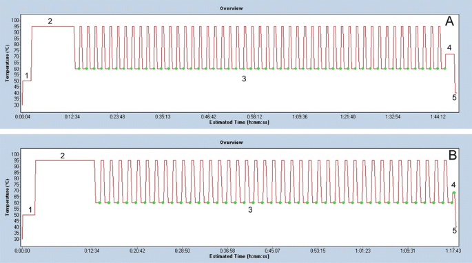

    

    Obtaining a shorter cycling time by editing the cycling conditions of another experiment. (a) Overview of a 50-cycle assay that finishes in 1 h 44 min 12 s. (b) Overview of another assay with fewer (40) cycles obtained by editing (a) and it finishes in 1 h 17 min 43 s, a gain of approximately 27 min (reproduced from author’s previous work [11])

  • (c) Open an existing object.

  • (d) Switch to other software modules such as the Navigator or the Tools section.

• 8. In the “Log on to” field, the last database selected on the computer is displayed by default (Example: In our laboratory, the experiment reported in this chapter is saved as “Staphylococci—Charles”). If several databases are available and you want to log on to a different database than the one displayed in the “Log on to” field, select the Options button. The Login dialog box expands to show a selection list of all available databases. Select a database from the list. The overview window has several areas loaded with different tasks and functions.

• 9. Click the Proceed sign to proceed with the login. The application now displays the LightCycler^® 480 Software Overview window containing the Status bar at the top, the Experiment Creation and Tasks area on the right, and the Global action bar on the extreme right.

  Understand the following areas of the Overview window:

  • (a) Status bar

    This area displays information about the currently active object and allows the user to select an object to view from a list of currently open objects. The fields in the Status bar and their functions are described below:

    • The User Field shows the name of the registered user currently logged on to the machine. This is made possible because every user registered on the machine has to sign in before performing any operation.

    • The Database Field shows the name and type of database to which the user is connected.

    • The Instrument Field shows the name and the operational status of the instrument the user is working on. Possible states include: Not Connected, Connected, Initializing, Standby (MWP loaded), Standby (No MWP), Running, and Error.

    • The Windows Field shows a pull-down menu listing all currently open windows. The pull-down menu enables the user to switch between windows.

  • (b) Module bar

    The Module bar, displayed on the left side of the screen, has six permanent buttons and their functions are described as follows:

    • The Experiment button opens the Run module including the experiment protocol, charts of experiment data, and notes entered by the logged in user running the experiment.

    • Subset Editor allows the user to group samples into subsets for analysis and for reports.

    • Analysis Button launches the Analyses Overview Window and enables the user to either create new analysis or open existing analyses.

    • The Report Button allows the user to define the contents of a report. It also enables viewing and printing of the report. However, the rule is that the Report Button is not active until an experiment is saved.

    • The Summary Button opens the summary module of the experiment containing information including the NAME, DATE, and OWNER of the experiment. It allows the user to save the experiment as a macro. A macro allows you to edit previous experiments and have them saved with new names. For instance, you can obtain a shorter cycling time by editing the cycling conditions of another experiment (Fig. 1) (see Note 9 ).

  • (c) Global action bar

    The Global action bar displayed on the right side of the screen contains buttons used for general software functions. Their availability depends on the active window currently opened.

• 10. Open About box button. Clicking this button opens the program’s About box, which contains shortcuts to the LC480 manuals in the installation folder and displays the software version and copyright information about the software.

• 11. Use the “Selection and Navigation Features” (see Note 10 ).

• 12. To create and execute a query, select the Query tab in the Navigator window. In the Object Type box, select the type of object to be retrieved. (Optional) Enter the name of the item to be retrieved or the owner of the item, if known. You may throw the wildcard “*” to search for any character string.

• 13. To create or modify an object (in the navigator), select Modification Date or Creation Date to specify which date you want to use in the query. The Modification Date and the Creation Date choices are mutually exclusive (i.e., you can search for one or the other, but not both). Select a date range for the search. You can specify the number of months or days before the current date or you can select a beginning and ending date in the past.

• 14. For any possible object type, you can also select a target folder from the Folders tab. Check the Scan Sub-folders box to include all subfolders within a directory in the search.

• 15. In using the navigation features, understand that the Roche folder contains some useful standard objects:

  • Demo experiments in the Experiments subfolder (see Note 11 ).

  • Demo run templates in the Templates subfolder including predefined subsets in the Subsets subfolder. The run templates folder contains templates for use with the LC480 instrument I or LC480 instrument II.

  • Color Compensation objects including the universal Color Compensation objects, and a demo melt object for Endpoint Genotyping analysis in the Special Data folder.

  • To modify a Roche object, you must first create a copy by exporting and importing it to your own user folder.

  • Administration folder that contains objects for user groups, user roles, user accounts, and security policies.

• 16. Click the Search button. Results are displayed in the pane to the right of the search criteria. The results include the following:

  • Object name.

  • Object type.

  • Date the object was created.

  • Date the object was last modified.

• 17. You can sort the result list in ascending or descending order by clicking the corresponding column head. If you select an object in the list, the full path to the object is displayed in the Status bar at the bottom of the Results pane. If the selected object is an experiment or a macro, a summary of object information is displayed in the Object Summary pane (see Note 12 ).

• 18. To open an object, double-click the object name.

• 19. Select and Deselect Samples. The Sample Selector is self-explanatory (see Note 13 ).

• 20. To set the selection status of enabled samples in the MWP image, click a sample to select it. Press the <Ctrl> key and click a selected sample to deselect it. If the MWP image and the Subset combo box are used together, selecting a subset enables only the samples in the subset and automatically selects them.

• 21. Click and drag on a deselected well to select all wells in the drag region. Press the <Ctrl> key and click and drag on a selected well to deselect all wells in the drag region.

• 22. Click row or column headers to select the corresponding rows or columns. Press the <Ctrl> key and click row or column headers to deselect the corresponding rows or columns. The display of the sample table corresponds to the selection of rows or columns in the sample selector.

• 23. Click the square in the upper left corner of the MWP image to toggle the selection status of the entire plate. If a legend is included in the Sample Selector you can use the Legend Property Selector to select which legend options are displayed. The options provided in the Legend Property Selector combo box depend on the context.

• 24. Click a colored icon in the legend to toggle the selection status of the corresponding wells. Selection of the legend icons is synchronized with the selection in the MWP image. A legend icon appears selected if all members of the group are selected in the MWP image. It will not appear selected if any group member is not checked.

• 25. Double-click a legend icon to select all items in the corresponding group and deselect all items not in the group.

• 26. To add wells to or remove them from a selection, press the <Ctrl> key and click a well, row, or column or click and drag a rectangle.

• 27. Scroll the MWP Image.

  The MWP image contains horizontal and vertical scroll bars to allow you to scroll and see any part of the image. When you are scrolling, the column and row headers remain fixed.

• 28. Zoom in and out of the MWP Image.

  You have several possibilities for zooming in on or out of the MWP image:

  • With the zoom buttons.

  • With the slider bars.

  • Manually setting the zoom by dragging the margins of a column or row.

  The MWP image provides two slider bars for zooming in a horizontal or vertical direction:

  • With the horizontal slider at the rightmost position (minimum zoom) the MWP image displays a single column.

  • With the horizontal slider at the leftmost position (maximum zoom) the MWP image displays all columns.

  • With the vertical slider at the topmost position (maximum zoom) the MWP image displays a single row.

  • With the vertical slider at the bottommost position (minimum zoom) the MWP image displays all rows.

  As well as zooming with the buttons or sliders, you can manually set the horizontal or vertical zoom by dragging the right margin of a column or the bottom margin of a row.

• 29. (Optional) Print the MWP Image

  The MWP image provides a Print button that allows you to print the visible section of the image. The print is scaled to a single page.

• 30. Use the Sample Table and Sample Selector to Select or Deselect samples for display in an analysis chart or to include/exclude a sample from analysis (see Note 14 ). You can select one or all of the samples in the Sample Table for display in an analysis chart, but you cannot change any of the information displayed. Selected samples are highlighted. To add or remove samples from the selection in the Sample Table, use the standard windows shift-click and ctrl-click features.

• 31. Include or Exclude Samples ( see Note 15 ). Further, samples can be included into or excluded from analysis. To include a sample, mark the Include box in the left table column. Status of the Include box is changed by double-clicking or by pressing the <Space> key. Using the Include option, you can, for instance, decide which standards are used to calculate the standard curve in Absolute Quantification analysis.

• 32. Export and Import Objects and Experiment Raw Data. To store objects outside the LC 480 Software database or to transfer objects between databases, you must export the LC 480 Software files (see Note 16 ).

• 33. For experiments you can also export the raw data in a tab-delimited text format (Experiment Text File (see Note 17 )).

• 34. To start the experiment run, click the Start Run button on the Run Protocol or the Data tab. You can only start an experiment run when an instrument is connected. The Start Run button is only available if a MWP has been loaded. You are prompted to save the experiment. Enter an experiment name and browse to a folder where you want to save the experiment. If you close the dialog without saving the experiment, the run will not start. A status bar on the Data tab indicates the progress of the running experiment (see Note 18 ).

• 35. To view data for specific samples, select one or more samples in the Sample Editor or Sample Table. If needed, you can modify chart settings during the experiment run.

• 36. (Optional) To adjust or stop the program during the run, click End Program to stop the current program and skip to the next program in the experiment protocol. Performing this task ensures that the data are complete and an analysis can be performed.

• 37. To stop the run, click the Abort Run button. (The Abort Run button replaces the Start Run button during the run.) Performing this task results in incomplete data, no analysis can be performed.

• 38. When the experiment is finished, a status message displays “Run complete.”

• 39. When the run is finished, open the plate loader again to remove the MWP. Hazard (see Note 19 ).

• 40. The next stage is the data analysis (see Note 20 ). Click Sample Editor in the Module bar to open the Sample Editor, and complete sample information, if necessary (see Note 21 ).

• 41. To perform an analysis, open the experiment you want to analyze in the LightCycler^® 480 Software main window.

• 42. In the Module bar, click Sample Editor. If you have not already entered sample information, enter information to identify the samples.

• 43. Enter the analysis-specific sample information. The kind of information you can enter depends on the type of analysis.

• 44. Click Analysis on the LightCycler^® 480 Software Module bar. The Analysis Overview window opens. The Analysis Overview window displays the Create New Analysis list and Open Existing Analysis list (if an analysis was created before).

• 45. Select the analysis type from the Create New Analysis list. The Create new analysis dialog opens. Here, you can again define the analysis type and select an analysis subset. If your experimental protocol should contain several programs that are suited for the selected analysis type, select one from the Program list. If you wish, you can change the analysis name (the default name is “analysis type for subset name”). Click the Proceed button (see Note 22 ).

• 46. In the Analysis window enter or adjust the parameters. Use the Color Compensation multi-select button to turn Color Compensation on or off and to select a Color Compensation object. Use the Filter Comb button to select the fluorescence channel you want to analyze.

• 47. Click Apply Template to display the Apply Template dialog box. Select a Template from the list and click the “proceed” button. The template settings are applied to the new experiment protocol.

• 48. Select the options specific to the analysis type. If you change information in the Sample Editor (except sample name, sample note, or target name) after performing the analysis, you must recalculate the analysis results using the updated values from the Sample Editor. In this case, the Calculate button becomes active again.

• 49. You can add more than one analysis to an experiment, including multiple instances of the same analysis type. Click the “add” in the Analysis toolbar.

• 50. Click the “save” button in the Global action bar to save the analysis results as part of the experiment.

• 51. To select samples to include or exclude in result calculations, select the checkbox next to a sample name to generate analysis results for the sample. By default, all samples are checked at the beginning of an analysis. Double-click a sample checkbox to deselect or reselect it. To check or uncheck a group of samples simultaneously, highlight the range of samples, and press the <Space> bar. This toggles the check marks on or off in all the selected sample boxes.

• 52. To select samples to view in charts, note the color of the sample in the sample list (samples are color-coded), and look for the color on the chart. Alternatively, place the mouse pointer over a line on a chart to display a small box containing the name of the sample represented by the line. When you highlight a sample name in the sample list, data from the selected sample is displayed in the analysis charts. By default, all samples are selected when you first open the analysis window.

• 53. You can redraw the analysis graphs using selected samples:

  • To select one sample, highlight the sample name in the sample list.

  • To select multiple samples, press the <Ctrl> key while clicking the sample names.

  • To select a contiguous set of samples, click the first sample name, and press the <Shift> key while clicking the last sample name in the set.

  • To select all samples, press <Ctrl-A>.

• 54. You can remove or rename analyses saved with your experiment if your user account has the Expert User or Local Administrator role. You may also be able to remove or rename analyses stored with experiments of other users, depending on the access privileges associated with your user account. To remove an analysis from an experiment:

  • Select an analysis from the Analyses bar.

  • Click the Remove Item button in the Analysis toolbar.

  • You are prompted to confirm your choice.

  • Click the Remove Item button in the Analysis toolbar to remove the analysis.

  • Click the Save Item button to save the experiment without the analysis.

• 55. You can rename the analysis associated with an experiment (renaming is helpful if you have more than one analysis of the same type associated with the experiment). Select an analysis from the Analyses bar. Click the Rename Item button in the Analysis toolbar. The Edit Name dialog opens. Enter a new name and click the Proceed button. (Remember: Names must be unique in each database folder).

• 56. Export analysis results (see Note 23 ). Click the Result Batch Export Navigator control button. The Batch Export wizard opens. On the Select Folders tab of the wizard, select a source folder in the Available Folders list and add it to the Selected Folders list. Check the Scan Sub-folders option to include all subfolders within the source directory.

• 57. On the Target tab, select the destination directory and the name of the output file. Click the Browse button to browse for a destination. Alternatively, type the path of the destination directly into the input field. If the specified output file already exists, the wizard will ask you to confirm before overwriting the existing file.

• 58. On the Analysis Type tab, select the type of analysis to be exported.

• 59. On the Start tab, you can review your settings and start the export process. The Reset button on the Start tab is active only after an export is complete. Clicking the Reset button resets the results of the previous export, so the export can be repeated.

• 60. On the Status tab, you can view the status of the export process. While the export is in progress, the Stop button is active. You can abort the export by clicking the Stop button.

• 61. The Done tab displays a summary of the batch export. Click the Done button to close the wizard. One of the key features of the LC480 system is that the software is designed to display detection signal(s) from one selected signal emission channel at any one time (Fig. 2). The LC480 system does not allow for simultaneous display of detection signals from all the emission channels (see Note 24 ).

  Fig. 2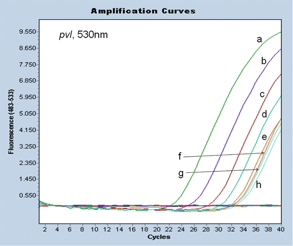

  

  Amplification curves for pvl detected via the FAM (530 nm) emission channel showing the fluorescence versus Cp for measured bacterial DNA load. 1.0 × 10⁷ CFU [Сp = 21.07] (a), 1.0 × 10⁶ CFU [Сp = 23.15] (b),1.0 × 10⁵ CFU [Сp = 26.28] (c), 1.0 × 10⁴ CFU [Cp = 29.25] (d), 1.0 × 10³ CFU [Cp = 32.90] (e),1.0 × 10² CFU [Cp = 33.03] (f),1.0 × 10¹ CFU [Cp = 33.32] (g), 1.0 CFU [Cp = 33.82] (h), respectively (reproduced from author’s previous work [11]

• 62. The analyzed data is now ready for presentation, publishing, or other uses.

4 Notes

• 1. If your laboratory has a biological safety cabinet (BSC) or microbiological safety cabinet (MSC) that has UV or Aircleaner, that would suffice.

• 2. The LC480 is described briefly. The LC480 instrument is available in two versions, one with a thermal block cycler for the LightCycler^® 480 MWP 96-wells, the other for the LightCycler^® 480 MWP 384-wells. Additionally, both LightCycler^® 480 Instrument versions are available with two different thermal block cyclers: LightCycler^® 480 Thermal Block Cycler Unit Silver and LightCycler^® 480 Thermal Block Cycler Unit Aluminum. Both thermal block cyclers can be used with LightCycler^® 480 Instrument I and II. Although you can purchase each version of the thermal block cycler as an exchangeable accessory (LightCycler^® 480 Block Kit 96 or 384), we recommend the 96 block for the large volume of reaction (40–50 μl) required for the heavy multiplexing described in this chapter. The 384 block is ideal for small volume (10–25 μl) monoplex reactions. We do not recommend interchanging the blocks because it often refuses releasing the holder. When it happens, calling the engineers is often not the best immediate solution as they would take time to get to the laboratory. Imagine losing the time, money, and materials invested in preparing a multiwall plate full of control and test samples. To circumvent this challenge, Roche later developed the 05015278001 version (96-well) and the 05015243001 version (384-well). Furthermore, following the launching of the LC480, alternative instruments capable of detecting DNA target through five floescent emission channels have joined the real-time PCR market—examples are the Rotorgene 6000 real-time PCR machine (Corbette, Australia) and the QuantStudio™ 6 and 7 Flex Real-Time PCR series (ThermoScientific, USA).

• 3. Besides the dyes listed in Table 1, all dyes that are compatible with the excitation and emission filter wavelengths can be measured by the LightCycler^® 480 Instrument I.

• 4. It is important to follow the safety instructions for handling biological fluids and tissues.

• 5. It is the tradition of life sciences experiments to run controls alongside test samples. In PCR many researchers tend to include “internal controls.” One commercial real-time PCR assay for PVL-MRSA that we operated clinical trials for (name withheld) was rubbished by the incorporation of an amplifiable internal control and oligonucleotides with which the internal control yielded amplification signal. However, we found that whenever CoNS was assayed, all the channels in the assay failed to detect the anticipated product (signal). In this pentaplex real-time PCR assay, the oligonucleotides targeting the bacterial 16S rRNA gene serve the purpose of detecting this gene as a positive control for all wells containing bacterial DNA and it never failed in our hands. Diagnostic assay users are interested in assays that work not assays loaded with interfering substances called internal controls.

• 6. The LEDs are first signposts of instrument wellness or malfunction.

• 7. The instrument manual and the commands are loaded in the computer which is driven by the LC480 software. To continue with the operation, understanding the LightCycler^® 480 software and the user interface is necessary—reason: when the user understands the software that drives the instrument, then it is easy to perform successful experiments with the machine. LightCycler^® 480 Software controls the LightCycler^® 480 instrument using information you provide in an experiment protocol. Raw data gathered by the software during real-time online PCR monitoring can then be analyzed utilizing the various analysis software modules and their functionalities. In this configuration, all software components are preinstalled on the LightCycler^® 480 control unit connected to the LightCycler^® 480 instrument. Each configuration (instrument and connected control unit) functions as an independent system with its own databases and its own set of user accounts. The location and destination folder of the database engine and database files is usually predefined for the installation process. All data gathered by the LightCycler^® 480 System are stored in the database to guarantee security for the data and data integrity. No manipulation of stored data and no access to raw data are possible. Analysis and editing of data can only be done within the LightCycler^® 480 software. The user interface of the LightCycler^® 480 Software displays some common elements including buttons with defined functionality which you will find on nearly all software screens. Furthermore, general button design conventions imply the function behind each button by using specific button indicators. Placing the mouse pointer over an icon or button displays a short description of its function and its keyboard shortcut (if available).

• 8. From the Overview window, you can create a new experiment, create a new experiment from a macro or a template, open an existing object, or switch to other software modules such as the Navigator or the Tools section. Understand the following areas of the Overview window:

  • (a) Editor frame

    The Editor Frame is the central area where the modules are displayed. The frame may contain several sections that can be resized individually. You can resize a section by dragging the splitter bar on the border between two sections to hide or show the section. The arrows on the splitter bar indicate which area of the Editor frame will be affected. Clicking a splitter bar will hide the corresponding area.

  • (b) Message area

    The Message area displays status messages, errors and warnings. The Message area consists of the following parts:

    Alarm icon on the left: The color of this icon changes depending on the severity of the alert:

    • Gray = normal information.

    • Yellow = warning.

    • Red = alarm condition.

  • (c) Understand the “Text field in the middle.” The text field in the middle displays messages, including the type, date, and time of message and the message text. Right-click a message entry to open the corresponding context menu. Select Show log in the context menu to display the log file and open the Error Log tool. Select Clear selected Messages to delete the selected messages from the Message area. Select Clear Messages to delete all messages from the Message area. Double-click a message entry or select Details in the context menu to display detailed information.

• 9. The temperature regime was a continuous flow that could be shown to consist of the five distinct steps outlined below:

  • Step 1 was a single cycle of 2 min at 50 °C for UNG.

  • Step 2 comprised a single cycle of 10 min at 95 °C (initial template denaturation and activation of polymerase).

  • Step 3 comprised 40 cycles of two-temperature cycling consisting of 15 s at 95 °C for initial template denaturation and 40 s at 60 °C for amplification (annealing and polymerization) with acquisition of fluorescence signal at 60 °C.

  • Step 4 was a single stage of 5 s at 68 °C for maximum signal acquisition from all the channels, as observed from the results of the CC object.

  • At step 5, the system cooled down to 40 °C for 5 s for the plate to be removed while the data was ready for analysis.

• 10. This section describes the object selection, navigation, and query elements of the LightCycler^® 480 Software:

  • Navigator

    The Navigator is similar, but not identical to the Windows Explorer of your computer. The Navigator displays data that are stored in a database not in the Windows file system. The Navigator window provides access to items stored in the LightCycler^® 480 database. Items include experiments, user accounts, instrument, macros, etc. The Navigator allows you to open experiments and related items (such as preferences, macros, and special data) as discrete objects. All items in the Navigator are organized in folders in a tree-like structure (similar to Windows Explorer) and are sorted alphabetically within their folders. You can expand and contract folder views and highlight the object you want to select. In addition, you can use the Query tab to search for specific LightCycler^® 480 Software objects in the database by entering search parameters.

    The Navigator window is structured into four areas:

    • 1. Tree pane.

    • 2. Object summary pane.

    • 3. Navigator controls.

    • 4. Query tab.

  Tree Pane

  The Navigator Tree pane displays a hierarchical tree view of the objects stored in the currently active database. The top object in the tree is always “Root.” The tree is used in a similar manner as for Windows Explorer. The Navigator Tree pane always includes the following default folders and objects:

  • User folders (including the System Admin folder and folders for each user account).

  • Each user folder contains default subfolders, such as a folder for experiments.

  • Roche folder that contains experiments, templates, and macros from Roche that can be used by anyone with access to LightCycler^® 480 Software.

  • To show or hide items under a folder, double-click the folder name or click the plus (+) or minus (−) sign next to the folder. Right-clicking an object in the Tree pane opens a context menu with the actions currently available for the object. For more information on the actions, see section Navigator Controls.

  Object Summary Pane

  The Navigator Object Summary pane displays experiment summary data if the currently selected object is an experiment or a macro.

  Navigator Controls

  In combination with the Tree pane, the Navigator control buttons allow you to work with objects in the database and to import and export objects. The buttons of the navigator Controls and their functions are described. The availability of the Navigator control buttons depends on your user role and on the database you have logged onto. A research database allows experiments and experiment-related objects to be renamed, deleted, or copied. With a traceable database this is not allowed. But it is possible to rename and delete templates and empty folders.

  Query Tab

  LightCycler^® 480 Software includes a query tool you can use to retrieve experiments and other objects stored in the LightCycler^® 480 Software database. The query tool is accessible via the Navigator in the form of the Query tab.

• 11. If your LC480 instrument is a new one, this subfolder provides templates for you to edit and kick start your own experiments.

• 12. If an error message is displayed stating that the query engine needs to be updated, you must update the database. If you have Local Administrator privileges, see “Updating the database” in section Administrative Tools for instructions. Otherwise, see your system administrator.

• 13. The Sample Selector and the Sample Table are displayed in many windows (example: most windows connected to analyses) in the LC480 Software. The Sample Selector includes a MWP image with selectable wells and a legend showing selectable sample groups where required. The MWP image can be used to select samples, or as a visual display. When used to select samples, it may appear with or without the legend and may also appear with or without a Sample Table. Samples in the MWP image can be enabled or disabled by choosing a subset in the Subset combo box. A disabled sample is colored dark gray, exhibits no response when clicked, and shows no information. Samples in the MWP that do not belong to the subset chosen for analysis are disabled by default and cannot be changed. Which sample groups are available in the legends depends on the analysis type. When enabled, a sample may be either selected or deselected. A selected sample is displayed as a pressed button with a white background. A button for a deselected sample is displayed as not pressed with a light blue background. Only selected samples are displayed in the Results table and on the corresponding analysis chart.

• 14. The sample color in the Sample Table always refers to the color in a chart or data display and to the color in the MWP image. Only samples that are enabled and selected in the Sample Selector are displayed in the Sample Table. Other information (in additional columns) may be added to a Sample Table according to the context of the screen (e.g., results such as Cp and concentration for quantification analyses). If there are more samples than can be displayed, a scroll bar is added. The Sample Selector and the Sample Table are displayed on many windows (example: most windows connected to analyses) in the LightCycler^® 480 Software and are used to select the samples to be displayed in the corresponding analysis charts or to include or exclude samples from analysis. For more information on the Sample Selector, see the previous section. The Sample Table displays the well coordinates of the samples in the MWP image and the color which represents a sample in the analysis charts (defined by the sample preferences).

• 15. After you have changed the include status of a sample, you must always recalculate the analysis.

• 16. Exporting a file does not remove the object from the database, but instead copies the file and stores it at the location you designate. The exported file has an .ixo file extension. You can also export any object in XML format as a Summary XML file. You can export the following objects:

  • User default preferences and user preferences for charts and samples.

  • LightCycler^® 480 experiments.

  • Standard melting curve.

  • Standard curve object.

  • Templates.

  • Macros.

  • Color Compensation objects.

  • LightCycler^® 480 Instrument Error and Operation logs.

• 17. The Experiment Text File format is tab-delimited. It includes two header lines:

  • The first header line contains the experiment name.

  • The second header line contains column headers.

  The data file contains the following information:

  • Sample position.

  • Sample name.

  • Program number.

  • Segment number.

  • Cycle number.

  • Acquisition time.

  • Acquisition temperature.

  • Fluorescence data for each channel.

• 18. As the experiment progresses, the Messages area displays messages indicating information, warnings, and errors encountered during the run. Returned sample data is displayed in the charts on the Data tab.

• 19. Directly after completion of a run, the MWP loader may be hot enough to cause an immediate burn. Wait an appropriate time period to let the loader cool down. Always include a final cooling step in your LightCycler^® 480 Instrument run protocol. Be aware that in case of a long standby the MWP itself may be heated to +60 to +80 °C by the heated lid, even if you have cooled down the LightCycler^® 480 Instrument to +40 °C after the PCR.

• 20. During a run, temporary backup data for the current experiment is saved to the user’s file system. If the run finishes and has saved the data in the database without an error, these temporary backup data are deleted. If the connection between the application and the instrument is temporarily interrupted, the software will download data automatically from the instrument after the connection is reestablished. The maximum length of a timeout is 7 min. If the timeout is exceeded, the run is considered prematurely terminated, and a warning is generated. If backup or instrument data exist, the data will be automatically recovered upon your next login or start of a new run if a corresponding experiment is found by the software. If no corresponding experiment is found, the software prompts you to confirm the deletion of the data.

• 21. You can enter or modify the sample information at any time before, during, or after the experiment is completed. We recommend that you enter the sample information before running the experiment.

• 22. You cannot make changes to an analysis subset after an analysis is created using the subset.

• 23. LightCycler^® 480 Software includes a batch export tool that lets you export all analysis results from experiments in a group of folders and all its subfolders by using the analysis batch result wizard. Follow the instructions below to export an experiment analysis. A result batch export exports all results of a selected analysis type from all experiments in a group of selected folders or experiments and all of the subfolders at the same time. The results are exported to a single tab-delimited file. Analysis result batch export is only possible from the Navigator. Analysis result batch export is performed using a wizard. You can move from a wizard step to the previous or next step by clicking the corresponding button. Note that the Next button will only be available when you have provided the settings required for the current tab.

• 24. Unlike some other real-time PCR machines that are able to display the signals from all detection channels simultaneously, the LC480 user cannot view more than one detection channel at a time, example; FAM (533 nm) channel at the same time as the LCR610 (610 nm) channel. For instance, some other machines including the ABI 7500 real-time PCR system [10] allow the user to view the signals from a selection of one, two, or all three channels. Each manufacturer of real-time PCR machines has some advantages over the other. No one machine manufacturer merits all the advantages.

References

Vu BN, Jafari AJ, Aardema M, Tran HK, Nguyen DN, Dao TT, Nguyen TV, Tran TK, Nguyen CK, Fox A, Bañuls AL, Thwaites G, Nguyen KV, Wertheim HF (2016) Population structure of colonizing and invasive Staphylococcus aureus strains in northern Vietnam. J Med Microbiol 65(pt 4):298–305. doi:10.1099/jmm.0.000220
Kolawole DO, Adeyanju Al, Schaumburg F, Akinyoola AL, Lawal OO, Amusa YB, Köck R, Becker K (2013) Characterization of colonizing Staphylococcus aureus isolated from surgical wards’ patients in a Nigerian university hospital. PLoS One 8(7):e68721. doi:10.1371/journal.pone.0068721
Ubukata K, Nakagami S, Nitta A, Yamane A, Kawakami S, Sugiura M, Konno M (1992) Rapid detection of the mecA gene in methicillin-resistant staphylococci by enzymatic detection of polymerase chain reaction products. J Clin Microbiol 30:1728–1733
Murakami K, Nomura K, Doi M, Yoshida T (1989) Production of low-affinity penicillin-binding protein by low- and high-resistance groups of methicillin-resistant Staphylococcus aureus. Antimicrob Agents Chemother 32:1307–1311
Foster TJ, Geoghegan JA, Ganesh VK, Hook M (2013) Adhesion, invasion and evasion: the many functions of the surface proteins of Staphylococcus aureus. Nat Rev Microbiol 12(1):49–62
Chambers HF (2005) Community-associated MRSA—resistance and virulence converge. N Engl J Med 352:1485–1487
David, M.Z., and Daum, R.S (2010) Community-associated methicillin-resistant Staphylococcus aureus: epidemiology and clinical consequences of an emerging epidemic. Clin Microbiol Rev 23(3), 616–687.
Geha DJ, Uhl JR, Gustaferro CA, Persing DH (1994) Multiplex PCR for identification of methicillin-resistant staphylococci in the clinical laboratory. J Clin Microbiol 32(7):1768–1772
Okolie CE, Wooldridge KG, Turner DP, Cockayne A, James R (2015a) Development of a heptaplex PCR assay for identification of Staphylococcus aureus and CoNS with simultaneous detection of virulence and antibiotic resistance genes. BMC Microbiol 15:157
Roche Applied Science. The LightCycler® 480 real-time PCR system catalogue. https://lifescience.roche.com/wcsstore/RASCatalogAssetStore/Articles/05237645001_10.12.pdf. Accessed 4 Apr 2016
Okolie CE (2009) Development of diagnostic and therapeutic tools for Staphylococcus aureus infections. Ph.D. Thesis, University of Nottingham. http://ethos.bl.uk/OrderDetails.do?uin=uk.bl.ethos.517830
Okolie CE, Wooldridge KG, Turner DP, Cockayne A, James R (2015b) Development of a new pentaplex real-time PCR assay for the identification of poly-microbial specimens containing Staphylococcus aureus and other staphylococci, with simultaneous detection of staphylococcal virulence and methicillin resistance markers. Mol Cell Probes 29(3):144–150
Johnsson DP, Stralin MK, Soderquist B (2004) Detection of Panton-valentine leukocidin gene in Staphylococcus aureus by LightCycler PCR: clinical and epidemiological aspects. Clin Microbiol Infect 10:884–889
Louie L, Goodfellow J, Mathieu P, Glatt A, Louie M, Simor AE (2002) Rapid detection of methicillin-resistant staphylococci from blood culture bottles by using a multiplex PCR assay. J Clin Microbiol 40(8):2786–2790
Author information
Authors and Affiliations
Corresponding author
Editor information
Editors and Affiliations
Rights and permissions
Copyright information
© 2017 Springer Science+Business Media LLC
About this protocol
Cite this protocol
Okolie, C.E. (2017). Real-Time PCR to Identify Staphylococci and Assay for Virulence from Blood. In: Bishop-Lilly, K. (eds) Diagnostic Bacteriology. Methods in Molecular Biology, vol 1616. Humana Press, New York, NY. https://doi.org/10.1007/978-1-4939-7037-7_12
Download citation
DOI: https://doi.org/10.1007/978-1-4939-7037-7_12
Published:
Publisher Name: Humana Press, New York, NY
Print ISBN: 978-1-4939-7035-3
Online ISBN: 978-1-4939-7037-7
eBook Packages: Springer Protocols