Probability and Random Variables

Abstract

Most signals we deal with in practice are random (unpredictable or erratic) and not deterministic. Random signals are encountered in one form or another in every practical communication system. They occur in communication both as information-conveying signal and as unwanted noise signal.

Philosophy is a game with objectives and no rules. Mathematics is a game with rules and no objectives.

—Anonymous

Problems

• 2.1 An experiment consists of throwing two dice simultaneously. (a) Calculate the probability of having a 2 and a 5 appearing together. (b) What is the probability of the sum being 8.

• 2.2 A circle is split into ten equal sectors which are numbered 1–10. When the circle is rotated about its center, a pointer indicates where it stops (like a wheel of fortune). Determine the probability: (a) of stopping at number 8, (b) of stopping at an odd number, (c) of stopping at numbers 1, 4, or 6, (d) of stopping at a number greater than 4.

• 2.3 A jar initially contains four white marbles, three green marbles, and two red marbles. Two marbles are drawn randomly one after the other without replacement. (a) Find the probability that the two marbles are red. (b) Calculate the probability that the two marbles have marching colors.

• 2.4 The telephone numbers are selected randomly from a telephone directory and the first digit (k) is observed. The result of the observation for 100 telephone numbers is shown below.

  k	0	1	2	3	4	5	6	7	8	9
  Nk	0	2	18	11	20	13	19	15	1	1

  What is the probability that a phone number: (a) starts with 6? (b) begins with an odd number?

• 2.5 A class has 50 students. Suppose 20 of them are Chinese and 4 of the Chinese students are female. Let event A denote “student is Chinese” and event B denote “student is female.” Find: (a) P(A), (b) P(AB), (c) P(B∣A).

• 2.6 In a particular city, voters registration follows the tabulated statistics below. What is the probability that a person selected at random will be a male given that the person is also a Republican?

  	Male (%)	Female (%)
  Democrat	26	28
  Republican	20	13
  Independent	12	12

• 2.7 For three events A, B, and C, show that

  $$ P\left(A+B+C\right)=P(A)+P(B)+P(C)-P(AB)-P(AC)-P(BC)+P\left( AB C\right) $$

• 2.8 A continuous random variable X has the following PDF

  $$ {f}_X(x)=\left\{\begin{array}{c}\hfill kx,\begin{array}{cc}\hfill \hfill & \hfill 1<x<4\hfill \end{array}\hfill \\ {}\hfill 0,\begin{array}{cc}\hfill \hfill & \hfill \mathrm{otherwise}\hfill \end{array}\hfill \end{array}\right. $$

  • (a) Find the value of constant k.

  • (b) Obtain F_X(x).

  • (c) Evaluate P(X ≤ 2.5) .

• 2.9 A random variable has a PDF given by

  $$ {f}_X(x)=\left\{\begin{array}{c}\hfill \frac{1}{2\sqrt{x}},\begin{array}{cc}\hfill \hfill & \hfill 0<x<1\hfill \end{array}\hfill \\ {}\hfill 0,\begin{array}{cc}\hfill \hfill & \hfill \mathrm{otherwise}\hfill \end{array}\hfill \end{array}\right. $$

  Find the corresponding F_X(x) and P(0.5 < x < 0.75).

• 2.10 A Cauchy random variable X has PDF

  $$ {f}_X(x)=\frac{1}{\pi \left(1+{x}^2\right)},\begin{array}{cc}\hfill \hfill & \hfill -\infty <x<\infty \hfill \end{array} $$

  Find the corresponding CDF.

• 2.11 A joint PDF is given by

  $$ {f}_{XY}\left(x,y\right)=k{e}^{-\left(2x+3y\right)/6}u(x)u(y) $$

  • (a) Determine the value of the constant k such that the PDF is valid.

  • (b) Obtain the corresponding CDF F_XY(x,y).

  • (c) Calculate the marginal PDFs f_X(x) and f_Y(y).

  • (d) Find P(X ≤ 3, Y > 2) and P(0 < X < 1, 1 < Y < 3).

• 2.12 X and Y are random variables which assume values 0 and 1 according to the probabilities in the table below. Find Cov(X,Y).

  X
  		0	1	Total
  Y	0	0.3	0.4	0.7
  	1	0.1	0.2	0.3
  	Total	0.4	0.6	1.0

• 2.13 The random variables X and Y have joint PDF as

  $$ {f}_{XY}\left(x,y\right)=\left\{\begin{array}{c}\hfill \frac{1}{4},\begin{array}{cc}\hfill \hfill & \hfill 0<x<2,\begin{array}{cc}\hfill \hfill & \hfill 0<y<2\hfill \end{array}\hfill \end{array}\hfill \\ {}\hfill 0,\begin{array}{cc}\hfill \hfill & \hfill \mathrm{otherwise}\hfill \end{array}\hfill \end{array}\right. $$

  Find: (a) E[X + Y], (b) E[XY].

• 2.14 Given that a is a constant, show that

  • (a) $\mathsf{Var}\left(\mathit{\mathsf{a}\mathsf{X}}\right)={\mathit{\mathsf{a}}}^2\mathsf{Vax}\left(\mathsf{X}\right)$

  • (b) $\mathrm{Var}\left(\mathrm{X}+\mathrm{a}\right)=\mathrm{Var}\left(\mathrm{X}\right)$

• 2.15 If X and Y are two independent random variables with mean ${\mu}_{\mathit{\mathsf{X}}}\ \mathsf{and}\ {\mu}_{\mathsf{Y}}$ and variances ${\sigma}_{\mathit{\mathsf{X}}}^2\kern0.5em \mathsf{and}\ {\sigma}_{\mathsf{y}}^2$ respectively, show that

  $$ \mathsf{Var}\left[\mathit{\mathsf{X}\mathsf{Y}}\right]={\sigma}_{\mathit{\mathsf{X}}}^2{\sigma}_{\mathit{\mathsf{y}}}^2+{\sigma}_{\mathit{\mathsf{X}}}^2{\mu}_{\mathit{\mathsf{y}}}^2+{\mu}_{\mathit{\mathsf{X}}}^2{\sigma}_{\mathit{\mathsf{y}}}^2 $$

• 2.16 Let $\mathit{\mathsf{f}}\left(\mathit{\mathsf{x}}\right)=\left\{\begin{array}{c}\hfill {\mathit{\mathsf{e}}}^{-\alpha \mathit{\mathsf{x}}}\left(\beta \mathit{\mathsf{x}}+\gamma \right),\begin{array}{cc}\hfill \hfill & \hfill \mathit{\mathsf{x}}>0\hfill \end{array}\hfill \\ {}\hfill 0,\begin{array}{cc}\hfill \hfill & \hfill \hfill \end{array}\mathsf{otherwise}\hfill \end{array}\right.$

  Find the conditions for α, β, and γ so that f(x) is a probability density function.

• 2.17 Given the joint PDF of random variables X and Y as

  $$ {f}_{XY}\left(x,y\right)=\left\{\begin{array}{c}\hfill \frac{1}{2}\left(x+3y\right),\begin{array}{cc}\hfill \hfill & \hfill 0<x<1,\begin{array}{cc}\hfill \hfill & \hfill 0<y<1\hfill \end{array}\hfill \end{array}\hfill \\ {}\hfill \kern-22pt 0,\begin{array}{cc}\hfill \hfill & \hfill \mathrm{otherwise}\hfill \end{array}\hfill \end{array}\right. $$

  • (a) Find E[X + Y] and E[XY].

  • (b) Calculate Cov(X,Y) and ρ_XY.

  • (c) Are X and Y uncorrelated? Are they orthogonal?

• 2.18 The joint PDF of two random variables X and Y is

  $$ {f}_{XY}\left(x,y\right)=y{e}^{-y\left(x+1\right)}u(x)u(y) $$

  • (a) Find the marginal PDFs f_X(x) and f_Y(y).

  • (b) Are X and Y independent?

  • (c) Calculate the mean and variance of X.

  • (d) Determine P(X < Y).

• 2.19 Given the joint PDF

  $$ {f}_{XY}\left(x,y\right)=\left\{\begin{array}{c}\hfill k\left(x+ xy\right),\begin{array}{cc}\hfill \hfill & \hfill 0<x<2,\begin{array}{cc}\hfill \hfill & \hfill 0<y<2\hfill \end{array}\hfill \end{array}\hfill \\ {}\hfill \kern-28pt 0,\begin{array}{cc}\hfill \hfill & \hfill \mathrm{otherwise}\hfill \end{array}\hfill \end{array}\right. $$

  • (a) Evaluate k.

  • (b) Determine P(X < 1, y > 1).

  • (c) Find F_XY(0.5,1.5).

  • (d) Obtain F_Y(y∣X = x).

  • (e) Calculate Cov(X,Y).

• 2.20 The skew is defined as the third moment taken about the mean, i.e.

  $$ \mathrm{skew}(X)=E\left[{\left(X-{m}_x\right)}^3\right]={\displaystyle \underset{-\infty }{\overset{\infty }{\int }}{\left(x-{m}_x\right)}^3}\kern0.30em {f}_X(x) dx $$

  Given that a random variable X has a PDF

  $$ {f}_X(x)=\left\{\begin{array}{c}\hfill \frac{1}{6}\left(8-x\right),\begin{array}{cc}\hfill \hfill & \hfill 4<x<10\hfill \end{array}\hfill \\ {}\hfill 0,\begin{array}{cc}\hfill \hfill & \hfill \mathrm{otherwise}\hfill \end{array}\hfill \end{array}\right. $$

  find skew(X).

• 2.21 Refer to the previous problem for the definition of skewness. Calculate skew(X), where X is a random variable with the following distributions:

  • (a) Binomial with parameters n and p

  • (b) Poisson with parameter λ.

  • (c) Uniform on the interval (a,b).

  • (d) Exponential with parameter α.

• 2.22 There are four resistors in a circuit and the circuit will fail if two or more resistors are defective. If the probability of a resistor being defective is 0.005, calculate the probability that the circuit does not fail.

• 2.23 Let X be a binomial random variable with p = 0.5 and n = 20. Find P(4 ≤ X ≤ 7).

  Hint: P(4 ≤ X ≤ 7) = P(X = 4) + P(4 < X ≤ 7).

• 2.24 The occurrence of earthquakes can be modeled by a Poisson process. If the annual rate of occurrence of earthquakes in a particular area is 0.02, calculate the probability of having exactly one earthquake in 2 years.

• 2.25 The number of cars arriving at a toll booth during any time interval T (in minutes) follows Poisson distribution with parameter T/2. Calculate the probability that it takes more than 2 min for the first car to arrive at the booth.

• 2.26 A uniform random variable X has E[X] = 1 and Var(X) = 1/2. Find its PDF and determine P(X > 1).

• 2.27 Two independent random variables are uniformly distributed, each having the PDF shown in Fig. 2.18. (a) Calculate the mean and variance of each. (b) Determine the PDF of the sum of the two random variables.

  Fig. 2.18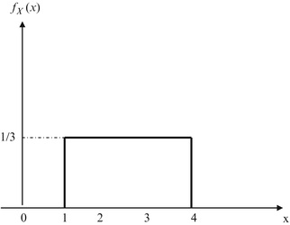

  

  For Prob. 2.27

• 2.28 A continuous random variable X may take any value with equal probability within the interval range 0 to α. Find E[X], E[X²], and Var(X).

• 2.29 A random variable X with mean 3 follows an exponential distribution. (a) Calculate P(X < 1) and P(X > 1.5). (b) Determine λ such that P(X < λ) = 0.2.

• 2.30 A zero-mean Gaussian random variable has a variance of 9. Find a such that P(∣X∣ > a) < 0.01.

• 2.31 A random variable T represents the lifetime of an electronic component. Its PDF is given by

  $$ {f}_T(t)=\frac{t}{\alpha^2} \exp \left[-\frac{t^2}{\alpha^2}\right]u(t) $$

  where α = 10³. Find E[T] and Var(T).

• 2.32 A measurement of a noise voltage produces a Gaussian random signal with zero mean and variance 2 × 10⁻¹¹ V². Find the probability that a sample measurement exceeds 4 μV.

• 2.33 A random variable has triangular PDF as shown Fig. 2.19. Find E[X] and Var(X).

  Fig. 2.19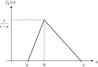

  

  For Prob. 2.33

• 2.34 A transformation between X and Y is defined by Y = e ^− 3X. Obtain the PDF of Y if:

  (a) X is uniformly distributed between −1 and 1, (b) f _X (x) = e ^− x u(x).

• 2.35 If ${f}_X(x)=\alpha {e}^{-\alpha x,},\begin{array}{cc}\hfill \hfill & \hfill \hfill \end{array}0<x<\infty$ and Y = 1/X, find f_Y(y).

• 2.36 Let X be a Gaussian random variable with mean μ and variance σ². (a) Find the PDF of Y = e ^X. (b) Determine the PDF of Y = X².

• 2.37 If X and Y are two independent Gaussian random variables each with zero mean and the same variance σ, show that random variable $R=\sqrt{X^2+{Y}^2}$ has a Rayleigh distribution as shown Fig. 2.20. Hint: The joint PDF is f _XY (x,y) = f _X (x)f _Y (y) and ${f}_R(r)=\frac{r}{\sigma^2}{e}^{-{r}^2/2{\sigma}^2}u(r)$.

  Fig. 2.20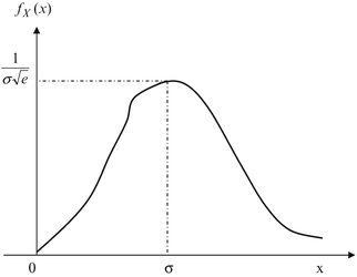

  

  PDF of a Rayleigh random variable for Prob. 2.37

• 2.38 Obtain the generating function for Poisson distribution.

• 2.39 A queueing system has the following probability of being in state n (n = number of customers in the system)

  $$ {p}_n=\left(1-\rho \right){\rho}^n,\begin{array}{cc}\hfill \hfill & \hfill n=0,1,2,\cdots \hfill \end{array} $$

  (a) Find the generating function G(z). (b) Use G(z) to find the mean number of customers in the system.

• 2.40 Use MATLAB to plot the joint PDF of random variables X and Y given by

  $$ {f}_{XY}\left(x,y\right)= xy{e}^{-\left({x}^2+{y}^2\right)},\begin{array}{cc}\hfill \hfill & \hfill \hfill \end{array}0<x<\infty, 0<y<\infty $$

  Limit x and y to (0,4).

• 2.41 Use MATLAB to plot the binomial probabilities

  $$ P(k)=\left(\begin{array}{c}\hfill k\hfill \\ {}\hfill n\hfill \end{array}\right){2}^{-k} $$

  as a function of n for: (a) k = 5, (b) k = 10.

• 2.42 Error in data transmission occurs due to white Gaussian noise. The probability of an error is given by

  $$ P=\frac{1}{2}\left[1-\mathrm{erf}(x)\right] $$

  where x is a measure of the signal-to-noise ratio. Use MATLAB to plot P over 0 < x <1.

• 2.43 Plot the PDF of Gaussian distribution with mean 2 and variance 4 using MATLAB.

• 2.44 Using the MATLAB command rand, one can generate random numbers uniformly distributed on the interval (0,1). Generate 10,000 such numbers and compute the mean and variance. Compare your result with that obtained using E[X] = (a + b)/2 and Var(X) = (b − a)²/12.

References

G. R. Grimmett and D.R. Stirzaker, Probability and Random Processes. Oxford: Oxford University Press, 2001, pp. 26–45.
X. R. Li, Probability, Random Signals, and Statistics. Boca Raton, FL: CRC Press, 1999, pp. 65–143.
R. Jain, The Art of Computer Systems Performance Analysis. New York: John Wiley & Sons, 1991, pp. 483–501.
R. Nelson, Probability, Stochastic Processes, and Queueing Theory. New York: Springer-Verlag, 1995, pp. 101–165.
P. G. Harrison and N. M. Patel, Performance Modelling of Communication Networks and Computer Architecture. Wokingham, UK: Addison-Wesley, 1992, pp. 19–48.
R. Goodman, Introduction to Stochastic Models. Mineola, NY: Dover Publications, 2nd ed., 2006.
O. C. Ibe, Markov Processes for Stochastic Modeling. Burlington, MA: Elsevier Academic Press, 2009.
Author information
Authors and Affiliations