Reaction Kinetics

Abstract

Chemical and biochemical networks can be viewed as dynamical systems. The properties of these systems can be complex and sometimes also surprising. Examples are enzyme kinetics, cells that interact and react to their environment by means of regulatory pathways, pattern on the skin of cows, leopards or snails are created by means of biochemical reactions, communication is done by biochemistry, to name but a few. All these very different systems can be modelled using the same basic principles.

Appendix: Reaction Kinetics

5.1.1 1 Solutions

5.1

• (a) Fast time scale (time t)

  $$\displaystyle\begin{array}{rcl} \frac{d} {dt}x& =& -(x - 2y^{3}) {}\\ \frac{d} {dt}\dot{y}& =& \varepsilon (x - y) {}\\ \end{array}$$

  Slow time scale $\tau =\varepsilon t$

  $$\displaystyle\begin{array}{rcl} \varepsilon \frac{d} {d\tau }x& =& -(x - 2y^{3}) {}\\ \frac{d} {d\tau }y& =& (x - y) {}\\ \end{array}$$

  Singular limit – fast system

  $$\displaystyle\begin{array}{rcl} \frac{d} {dt}x& =& -(x - 2y^{3}) {}\\ \frac{d} {dt}y& =& 0 {}\\ \end{array}$$

  Singular limit – slow system

  $$\displaystyle\begin{array}{rcl} 0& =& -(x - 2y^{3}) {}\\ \frac{d} {d\tau }y& =& (x - y) {}\\ \end{array}$$

• (b) Fast system and slow manifold: y is fixed; x(t) converges to 2y ³. The slow manifold reads

  $$\displaystyle{\{(x,y)\,\vert \,x = 2y^{3}\}.}$$

• (c) For the approximate equation, we replace x by an expression in y, assuming that we are on the slow manifold. Hence,

  $$\displaystyle{\frac{d} {d\tau }y = x - y = 2\,y^{3} - y.}$$

5.2 The basic equations for a, b and c read

$$\displaystyle\begin{array}{rcl} \dot{a}& =& -k_{1}b^{2}a + k_{ -1}c + k_{2}c {}\\ \dot{b}& =& -2k_{1}b^{2}a + 2k_{ -1}c {}\\ \dot{c}& =& k_{1}b^{2}a - k_{ -1}c - k_{2}c. {}\\ \end{array}$$

Using a + c = a ₀ yields

$$\displaystyle\begin{array}{rcl} \dot{b}& =& -2k_{1}b^{2}a_{ 0} + 2(k_{-1} + k_{1}b^{2})c {}\\ \dot{c}& =& k_{1}b^{2}a_{ 0} - (k_{1}b^{2} + k_{ -1} + k_{2})c. {}\\ \end{array}$$

The steady state assumption $\dot{c}$ leads to $c = \frac{k_{1}b^{2}a_{ 0}} {k_{1}b^{2}+k_{-1}+k_{2}}$ and

$$\displaystyle{\dot{b} = -2\dot{c} - 2k_{2}c = \frac{-2k_{2}k_{1}a_{0}b^{2}} {k_{1}b^{2} + k_{-1} + k_{2}}.}$$

The half maximum production is reached for $b = \sqrt{\frac{k_{-1 } +k_{2 } } {k_{1}}}$.

5.3

• (1) The case that one enzyme handles more than one substrate is quite common (e.g. in the coagulation system we shall consider). The simplest case is given, if there is only one active centre at the enzyme, and the two substrates compete for this active zone.

  $$\displaystyle\begin{array}{rcl} S_{1} + E& \mathop{\rightleftharpoons }\limits _{k_{-1}}^{k_{1}}& [S_{1}E]\mathop{\rightarrow }\limits ^{k_{2}}P_{1} + E {}\\ S_{2} + E& \mathop{\rightleftharpoons }\limits _{\tilde{k}_{-1}}^{\tilde{k}_{1}}& [S_{ 2}E]\mathop{\rightarrow }\limits ^{\tilde{k}_{2} }P_{1} + E {}\\ & & {}\\ \end{array}$$

  The model equations read

  $$\displaystyle\begin{array}{rcl} \quad [S_{1}]^{{\prime}}& =& k_{ 1}[S_{1}][E] + k_{-1}[S_{1}E] {}\\ \quad [S_{1}E]^{{\prime}}& =& k_{ 1}[S_{1}][E] + k_{-1}[S_{1}E] - k_{2}[S_{1}E] {}\\ \quad [P_{1}]^{{\prime}}& =& k_{ 2}[S_{1}E] {}\\ \quad [S_{2}]^{{\prime}}& =& \tilde{k}_{ 1}[S_{2}][E] +\tilde{ k}_{-1}[S_{2}E] {}\\ \quad [S_{2}E]^{{\prime}}& =& \tilde{k}_{ 1}[S_{2}][E] +\tilde{ k}_{-1}[S_{2}E] -\tilde{ k}_{2}[S_{2}E] {}\\ \quad [P_{2}]^{{\prime}}& =& \tilde{k}_{ 2}[S_{2}E] {}\\ \end{array}$$

• (2) This situation bears some similarity with the competitive inhibition considered above. We again assume all complex formations in equilibrium ($[S_{1}E]^{{\prime}} = 0 = [S_{2}E]^{{\prime}}$) and find from $[S_{1}E]^{{\prime}} = 0$, $[S_{2}E]^{{\prime}} = 0$

  $$\displaystyle{K_{m}^{1} = \frac{[S_{1}][E]} {[S_{1}E]},\quad K_{m}^{2} = \frac{[S_{2}][E]} {[S_{2}E]}.}$$

  The conservation law yields for the enzyme

  $$\displaystyle{E_{0} = [E] + [ES_{1}] + [ES_{2}].}$$

  Thus,

  $$\displaystyle{\frac{k_{2}^{1}[ES_{1}]} {E_{0}} = k_{2}^{1}\,\, \frac{[S_{1}][E]/K_{m}^{1}} {[E] + [ES_{1}] + [ES_{2}]} = k_{2}^{1}\,\, \frac{[S_{1}][E]/K_{m}^{1}} {[E] + [E][S_{1}]/K_{m}^{1} + [E][S_{2}]/K_{m}^{2}}}$$

  i.e.,

  $$\displaystyle{ \frac{d} {dt}[S_{1}] = -k_{2}^{1}\,\, \frac{[S_{1}]E_{0}/K_{m}^{1}} {1 + [S_{1}]/K_{m}^{1} + [S_{2}]/K_{m}^{2}}}$$

  and, similarly,

  $$\displaystyle{ \frac{d} {dt}[S_{2}] = -k_{2}^{2}\,\, \frac{[S_{2}]E_{0}/K_{m}^{2}} {1 + [S_{1}]/K_{m}^{1} + [S_{2}]/K_{m}^{2}}.}$$

• (3) From the reaction of the enzyme and substrate S ₁ alone (resp. the enzyme and the second substrate alone) we can conclude the behaviour of the mixture of all three substances. We may now perform a Lineweaver-Burk plot for substrate S ₁ alone ([S ₂] = 0), and one for substrate S ₂ alone ([S ₂] = 0). From these two plots, we are able to derive $k_{2}^{i}E_{0}$ and $K_{m}^{i}$ (with i = 1, 2).

5.4 The quasi-steady-state assumption and mass conservation leads to

$$\displaystyle\begin{array}{rcl} \frac{SE_{1}} {[SE_{1}]} = K_{m,1},\quad \frac{SE_{2}} {[SE_{2}]} = K_{m,2},\quad E_{1}^{0} = E_{ 1} + [SE_{1}],\quad E_{2}^{0} = E_{ 2} + [SE_{2}].& & {}\\ \end{array}$$

Thus,

$$\displaystyle\begin{array}{rcl} \frac{d} {dt}P& =& k_{2}[SE_{1}] +\hat{ k}_{2}[SE_{2}] = k_{2}\frac{[SE_{1}]E_{1}^{0}} {E_{1}^{0}} +\hat{ k}_{2}\frac{[SE_{2}]E_{2}^{0}} {E_{2}^{0}} {}\\ & =& k_{2} \frac{[SE_{1}]E_{1}^{0}} {E_{1} + [SE_{1}]} +\hat{ k}_{2} \frac{[SE_{2}]E_{2}^{0}} {E_{2} + [SE_{2}]} {}\\ & =& k_{2} \frac{SE_{1}E_{1}^{0}/K_{m,1}} {E_{1} + SE_{1}/K_{m,1}} +\hat{ k}_{2} \frac{S_{2}E_{2}E_{2}^{0}/K_{m,2}} {E_{2} + SE_{2}/K_{m,2}} {}\\ & =& k_{2} \frac{SE_{1}^{0}} {K_{m,1} + S} +\hat{ k}_{2} \frac{SE_{2}^{0}} {K_{m,2} + S} {}\\ \end{array}$$

The combined effect of two enzymes is just the sum of the effects due to the single enzymes.

5.5

• (1) The compartmental model reads

  $$\displaystyle\begin{array}{rcl} X^{{\prime}}& =& -K_{ 1}X + K_{2}Y {}\\ Y ^{{\prime}}& =& K_{ 1}X - K_{2}Y {}\\ \end{array}$$

  We find $(X + Y )^{{\prime}} = 0$, i.e., mass conservation.

• (2) We know that

  $$\displaystyle{X = v_{1}x,\quad Y = v_{2}y.}$$

  Thus,

  $$\displaystyle\begin{array}{rcl} & & v_{1}x^{{\prime}} = -K_{ 1}\,v_{1}x + K_{2}\,v_{2}y\qquad \Leftrightarrow \qquad x^{{\prime}} = -K_{ 1}x + K_{2}\frac{v_{2}} {v_{1}}y {}\\ & & v_{2}y^{{\prime}} = K_{ 1}\,v_{1}x - K_{2}\,v_{2}y\qquad \Leftrightarrow \ \qquad \ \ y^{{\prime}} = K_{ 1}\frac{v_{1}} {v_{2}}x - K_{2}y {}\\ \end{array}$$

  Mass conservation is expressed as

  $$\displaystyle{(v_{1}x + v_{2}y)^{{\prime}} = 0.}$$

• (3) Are the rate constants K ₁, K ₂ independent on v ₁? Let us first start with initial conditions x(0) = x ₀ > 0 and y(0) = 0. In a first, small time interval y is very small, and we may replace the full model by x ^′ = −K ₁ x, $y^{{\prime}} = K_{1}v_{1}x/v_{2}$. This is, the change of the concentration in the test tube is independent of the test tube, while the flow into the cell depends on the volume of the test tube (is proportional to v ₁). This is not what we want to see! The flow through the cell membrane at a point of time should only depend on the concentration outside of the cell membrane. We need to rescale K ₁. We have two possibilities:

  • (a) $k_{1} = K_{1}v_{1}/v_{2}$, k ₂ = K ₂. Then,

    $$\displaystyle\begin{array}{rcl} x^{{\prime}}& =& -k_{ 1}\frac{v_{2}} {v_{1}}x + k_{2}\frac{v_{2}} {v_{1}}y {}\\ y^{{\prime}}& =& k_{ 1}x - k_{2}y. {}\\ \end{array}$$

  • (b) $\tilde{k}_{1} = K_{1}\,v_{1}$, $\tilde{k}_{2} = K_{2}\,v_{2}$, with the consequence that

    $$\displaystyle\begin{array}{rcl} x^{{\prime}}& =& -\frac{\tilde{k}_{1}} {v_{1}} x + \frac{\tilde{k}_{2}} {v_{1}} y {}\\ y^{{\prime}}& =& \frac{\tilde{k}_{1}} {v_{2}} x -\frac{\tilde{k}_{2}} {v_{2}} y. {}\\ \end{array}$$

    While possibility (b) is more symmetric (and in this respect more satisfying), the rate constants in solution (a) carry more simple units (one over time), as expected in a linear compartmental model. Though the rate k ₁ implicitly depends on v ₂ (if we consider two cells of unequal volume we need to adapt k ₁, which is not the case in (b)), the simplicity of the units in (a) seems to be in favour of this variant.

• (4) Let E denote the number of non-occupied channels on the cell surface, and [XE] the number of channels actually involved in transportation of a ion. The total amount of channels is e ₀. We may write the transport as a chemical equation,

  $$\displaystyle{X + E\mathop{\rightleftharpoons }\limits _{\hat{k}_{-1}}^{\hat{k}_{1} }[XE]\mathop{\rightarrow }\limits ^{\hat{k}_{2} }Y + E.}$$

  The assumption that complex formation is at its equilibrium leads to

  $$\displaystyle{K_{m} = \frac{xe} {[XE]}}$$

  (note that we use the concentration x at this point); mass conservation for the channels implies e + [XE] = e ₀. Thus, the rate at which molecules appear in the interior of the cell is given by

  $$\displaystyle{\text{rate} =\hat{ k}_{2}[XE] = \frac{e_{0}\hat{k}_{2}[XE]} {e_{0}} = \frac{e_{0}\hat{k}_{2}[XE]} {e + [XE]} = \frac{e_{0}\hat{k}_{2}x/K_{m}} {1 + x/K_{m}}.}$$

  This rate replaces the expression k ₁ x in the linear model above. We obtain (with $k = e_{0}\hat{k}_{2}$)

  $$\displaystyle\begin{array}{rcl} x^{{\prime}}& =& -\frac{v_{2}} {v_{1}}\,\, \frac{kx} {K_{m} + x} + k_{2}\frac{v_{2}} {v_{1}}y {}\\ y^{{\prime}}& =& \frac{k\,x} {K_{m} + x} - k_{2}y. {}\\ \end{array}$$

• (5) Let us assume that $v_{1}x + v_{2}y = x_{0}v_{1}$, where the initial concentration x ₀ in the external volume is varied between different experiments. We measure the concentration within the cell (at equilibrium).

  (a) Linear model:

  $$\displaystyle\begin{array}{rcl} k_{1}x - k_{2}y& =& 0 {}\\ v_{1}x + v_{2}y& =& v_{1}x_{0} {}\\ \end{array}$$

  and hence

  $$\displaystyle{y = x_{0} \frac{k_{1}v_{1}} {k_{2}v_{1} + k_{1}v_{2}}.}$$

  This is, the concentration within the cell increases linearly with x ₀. (b) In the nonlinear case, the computation is more involving. We find

  $$\displaystyle\begin{array}{rcl} \frac{k\,x} {K_{m} + x} - k_{2}y& =& 0 {}\\ v_{1}x + v_{2}y& =& v_{1}x_{0} {}\\ \end{array}$$

  If x(0) is large and $v_{1} \gg v_{2}$, the concentration outside will not be changed a lot. This is, x(t) stays large. Thus, we approximate the Michaelis-Menten term

  $$\displaystyle{ \frac{k\,x} {K_{m} + x} \approx k}$$

  and obtain

  $$\displaystyle{y = k/k_{2}}$$

  independent on x ₀. In the linear case, the internal concentration depends linearly on x ₀, the initial concentration outside; the cell has no control at all about the internal concentration. In the Michaelis-Menten case, this is different: The internal equilibrium concentration is fairly independent on the change of concentration outside. The cell is able to control the internal concentration very well.

  Addendum: If we also use a Michaelis-Menten kinetics for the outflow, our model resembles the Goldbeter model. Dependent on the K _m -values characterising the ion channels we may either approximate the situations described above, or we may even find some strong nonlinear threshold behaviour.

5.6 The differential equations read

$$\displaystyle\begin{array}{rcl} \frac{dx} {dt} & =& x^{2}y - x + b {}\\ \frac{dy} {dt} & =& -x^{2}y + a. {}\\ \end{array}$$

The stationary state is $\left (a + b, \frac{a} {(a+b)^{2}} \right )$ and the Jacobian becomes

$$\displaystyle{J = \left (\begin{array}{cc} \frac{a-b} {a+b} & (a + b)^{2} \\ \frac{-2a} {a+b} & - (a + b)^{2} \end{array} \right ),}$$

with

$$\displaystyle\begin{array}{rcl} \beta & =& tr\,J = \frac{a - b} {a + b} - (a + b)^{2} {}\\ \gamma & =& det\,J = -(a - b)(a + b) + 2a(a + b) = (a + b)^{2} {}\\ \end{array}$$

Obviously, γ is always positive; when β = 0, then a bifurcation occurs, i.e., $\frac{a-b} {a+b} = (a + b)^{2}$, the eigenvalues are

$$\displaystyle{\lambda _{1,2} = \frac{\pm \sqrt{-4\gamma }} {2} = \pm (a + b)i}$$

The equations correspond to the phase plane diagram shown in Fig. 5.48

Fig. 5.48

Phase diagram for the modified Schnakenberg model

The nullclines satisfy following equations:

$$\displaystyle\begin{array}{rcl} \dot{x} = 0&:& y = \frac{x - b} {x^{2}}, {}\\ \dot{y} = 0&:& y = \frac{a} {x^{2}}. {}\\ \end{array}$$

Thus, there exists a finite region in the first quadrant which cannot be left by a trajectory. In this case, the theorem of Poincare-Bendixson yields the existence of a stable periodic orbits in case of the stationary state is unstable.

5.7 Obviously: The symmetry of the equations allows to find equilibrium solution(s) with all m _i equal. Thus, we look for a solution of

$$\displaystyle{E(p) = -p + \frac{\alpha } {1 + p^{n}} +\alpha _{0}.}$$

We find:

$$\displaystyle{E^{{\prime}}(p) = -1 + \frac{-n \cdot p^{n-1}\cdot \alpha } {(1 + p^{n})^{2}} <0,}$$

thus, E is monotone decreasing in p. Furthermore:

$$\displaystyle{E(0) =\alpha _{0}+\alpha> 0,\quad \lim p \rightarrow \infty E(p) \rightarrow -\infty }$$

thus, E(p) has exactly one positive root, denoted by $\tilde{p}$. So, it follows that there is exactly one equilibrium of the system with $m_{i} = p_{i} =\tilde{ p}$, i = 1, 2, 3.

Let us assume without loss of generality, that $p_{1}>\tilde{ p}$. Then, it follows:

$$\displaystyle{-p_{2} + \frac{\alpha } {1 + p_{1}^{n}} +\alpha _{0} = 0\quad \Leftrightarrow \quad \frac{\alpha } {1 + p_{1}^{n}} +\alpha _{0} = p_{2}\quad \leadsto p_{2} <\tilde{ p}}$$

In the next step:

$$\displaystyle{-p_{3} + \frac{\alpha } {1 + p_{2}^{n}} +\alpha _{0} = 0\quad \Leftrightarrow \quad \frac{\alpha } {1 + p_{2}^{n}} +\alpha _{0} = p_{3}\quad \leadsto p_{3}>\tilde{ p}}$$

In the next step:

$$\displaystyle{-p_{1} + \frac{\alpha } {1 + p_{3}^{n}} +\alpha _{0} = 0\quad \Leftrightarrow \quad \frac{\alpha } {+p_{3}^{n}} +\alpha _{0} = p_{1}\quad \leadsto p_{1} <\tilde{ p}}$$

which is a contradiction to the original assumption. Thus, further stationary states are not possible in that system.

5.8

• (a) This term corresponds to a permutation π ∈ S _n s.t. ∏ a _i, π(i) ≠ 0. As any permutation is a product of cycles, this fact is equivalent with the fact that every state is member of at least one feedback cycle. Only if we have a state that has (in the corresponding graph) either no incoming or no outgoing edge (or booth), we do not find such a permutation.

• (b.1) Let state x ₁ be a state with no outgoing edge. Then, x ₁ does not appear in any of the equations for x ₁,…,x _n . We may reduce the system to this smaller system. The state x ₁only couples to x ₂,…,x _n ,

  $$\displaystyle{\dot{x}_{1} = f_{1}(x_{2},\ldots,x_{n}).}$$

  If the subsystem does not exhibit bistability, the complete system is also not able to exhibit bistability.

• (b.2) Let state x ₁ have no incoming edge. Then,

  $$\displaystyle{x_{1} = \text{constant}}$$

  and x ₁ is either constant in time (if the prod constant is zero), or a linear function of time.

  In the first sub-case (x ₁ constant), we may remove x − 1as a (dynamic) state form the system, and interpret this state as a parameter. That is, no restriction.

In the second sub-case, x ₁ grows linearly in time. That is, we do not have any stationary states in the system. Also here, the restriction is not serious.

5.9

• (a) x _i : amount of mRNA coded by gene i, y _i : amount of protein coded by gene i.

  $$\displaystyle\begin{array}{rcl} x_{1}^{{\prime}}& =& \frac{\alpha _{1}} {1 + k_{1}y_{2}} -\gamma _{1,1}x_{1} {}\\ y_{1}^{{\prime}}& =& a_{ 1}x_{1} -\gamma _{1,2}y_{1} {}\\ x_{2}^{{\prime}}& =& \frac{\alpha _{2}} {1 + k_{2}y_{1}} -\gamma _{2,1}x_{2} {}\\ y_{2}^{{\prime}}& =& a_{ 2}x_{2} -\gamma _{2,2}y_{2} {}\\ \end{array}$$

• (b) We find negative loops of any state to itself; this is the diagonal of the Jacobian that is not of importance according to our new definition. Between states, we have only one (long) feedback loop

  $$\displaystyle{x_{1}\stackrel{+}{\rightarrow }y_{1}\stackrel{-}{\rightarrow }x_{2}\stackrel{+}{\rightarrow }y_{2}\stackrel{-}{\rightarrow }x_{1}}$$

  that is positive. Hence, our system is cooperative, if we choose the appropriate cone. Sign structure of the Jacobian:

  $$\displaystyle{J = \left (\begin{array}{cccc} -&0 & 0 &-\\ + &- & 0 & 0 \\ 0 &-&-&0\\ 0 & 0 &+ &- \end{array} \right )}$$

  We follow the lines of the proof for systems with positive feedbacks only: Take x ₁ as reference state. The states y ₁ can be reached by a positive path (path with even no of negative entries), x ₂ and y ₂ by a “negative” path (path with odd no of negative entries).

  We have already a “good” ordering, and the off-diagonal elements indeed have the Morishima-form,

  $$\displaystyle{J = \left (\begin{array}{cc|cc} {\ast} &0 & 0 &-\\ + & {\ast} & 0 & 0 \\ \hline 0&-&{\ast}&0\\ 0 & 0 &+ & {\ast} \end{array} \right )}$$

  In order to obtain a cooperative system, we should use the cone (+, +, −, −) as positive cone, i.e., use the transformation matrix

  $$\displaystyle{S = \left (\begin{array}{cc|cc} 1 &0& 0 & 0\\ 0 &1 & 0 & 0 \\ \hline 0&0& - 1& 0\\ 0 &0 & 0 & -1 \end{array} \right )\quad \Rightarrow \quad S^{-1}JS = \left (\begin{array}{cc|cc} {\ast} &0 & 0 &+\\ + & {\ast} & 0 & 0 \\ \hline 0&+& {\ast}&0\\ 0 & 0 &+ & {\ast} \end{array} \right )}$$

  We will tend to a stationary state, which is either $(x_{1},y_{1})$ high and $(x_{2},y_{2})$ low or vice versa.

  (see also: [79]. )

• (c) Direct generalisation, using a symmetrical design:

  $$\displaystyle\begin{array}{rcl} x_{1}^{{\prime}}& =& \frac{\alpha _{1}} {(1 + k_{1}y_{2})(1 +\tilde{ k}_{1}y_{3})} -\gamma _{1,1}x_{1} {}\\ y_{1}^{{\prime}}& =& a_{ 1}x_{1} -\gamma _{1,2}y_{1} {}\\ x_{2}^{{\prime}}& =& \frac{\alpha _{2}} {(1 + k_{2}y_{1})(1 +\tilde{ k}_{2}y_{3})} -\gamma _{2,1}x_{2} {}\\ y_{2}^{{\prime}}& =& a_{ 2}x_{2} -\gamma _{2,2}y_{2} {}\\ x_{2}^{{\prime}}& =& \frac{\alpha _{3}} {(1 + k_{3}y_{1})(1 +\tilde{ k}_{3}y_{2})} -\gamma _{3,1}x_{3} {}\\ y_{2}^{{\prime}}& =& a_{ 3}x_{3} -\gamma _{3,2}y_{3} {}\\ \end{array}$$

  We have negative feedback loops in the system, e.g.

  $$\displaystyle{y_{1} \rightarrow x_{2} \rightarrow y_{2} \rightarrow x_{3} \rightarrow y_{3} \rightarrow x_{1} \rightarrow y_{1}.}$$

  If we add additional nonlinearity (using inhibitory Hill-function with a hill-coefficient large enough) and appropriate parameter values will lead to oscillations in the system.

The solution is a hierarchical design:

$$\displaystyle\begin{array}{rcl} x_{1}^{{\prime}}& =& \frac{\alpha _{1}} {1 + k_{1}y_{2}} -\gamma _{1,1}x_{1} {}\\ y_{1}^{{\prime}}& =& a_{ 1}x_{1} -\gamma _{1,2}y_{1} {}\\ x_{2}^{{\prime}}& =& \frac{\alpha _{2}} {1 + k_{2}y_{1}} -\gamma _{2,1}x_{2} {}\\ y_{2}^{{\prime}}& =& a_{ 2}x_{2} -\gamma _{2,2}y_{2} {}\\ \tilde{x}_{1}^{{\prime}}& =& \frac{\tilde{\alpha }_{1}y_{2}} {1 + k_{1}\tilde{y}_{2}} -\tilde{\gamma }_{1,1}\tilde{x}_{1} {}\\ \tilde{y}_{1}^{{\prime}}& =& \tilde{a}_{ 1}\tilde{x}_{1} -\tilde{\gamma }_{1,2}\tilde{y}_{1} {}\\ \tilde{x}_{2}^{{\prime}}& =& \frac{\tilde{\alpha }_{2}y_{2}} {1 +\tilde{ k}_{2}\tilde{y}_{1}} -\tilde{\gamma }_{2,1}\tilde{x}_{2} {}\\ \tilde{y}_{2}^{{\prime}}& =& \tilde{a}_{ 2}\tilde{x}_{2} -\tilde{\gamma }_{2,2}\tilde{y}_{2} {}\\ \end{array}$$

The system $(x_{1},y_{1},x_{2},y_{2})$ is independent of the “tilde”-system, and hence cooperative. Asymptotically it will tend to a stationary state (exponentially fast). The we can use the theorem about eventually autonomous systems, and find that eventually the system $(\tilde{x}_{1},\tilde{y}_{1},\tilde{x}_{2},\tilde{y}_{2})$ becomes autonomous (and again cooperative). The value of y ₂ in its stationary state serves as a parameter. This parameter activates both “tilde”-genes. Hence the “tilde”-system may only come up if y ₂ is large. We have the three outcomes:

• (1) x ₁ high, x ₂ low, $\tilde{x}_{1}$ and $\tilde{x}_{2}$ low

• (2) x ₁ low, x ₂ high, $\tilde{x}_{1}$ high, $\tilde{x}_{2}$ low

• (3) x ₁ low, x ₂ high, $\tilde{x}_{1}$ low, $\tilde{x}_{2}$ high

5.10

• (a) First of all, there is no feedback from TNF into the regulatory system; hence, we do not need to take this variable into account.

x ₁ enhances the production of x ₂, which in turn enhances the production of x ₁. This is a positive feedback.

x ₁ enhances the production of y ₁ that suppresses x ₂ (which enhances x ₁). This is a negative feedback. We find a positive feedback in parallel with a negative feedback (see Fig. 5.49). The latter is assumed to react on a slow time scale.

Fig. 5.49

Structure of the model in Exercise 5.10

• (b) We assume the α(t) = 0. Now we analyse the system using time scale arguments.

The fast system reads

$$\displaystyle\begin{array}{rcl} \dot{x}_{1}& =& \beta _{2} \frac{x_{2}^{2}} {\hat{x}^{2} + x_{2}^{2}} -\gamma x_{1} {}\\ \dot{x}_{2}& =& \beta _{1}x_{1} -\gamma x_{2} -\eta \,\, y\,\,x_{2} {}\\ y& =& \text{constant}. {}\\ \end{array}$$

Thus, we have a positive feedback only, and find for the stationary states

$$\displaystyle{x_{2} = \frac{\beta _{1}} {\gamma +\eta y}\,x_{1}.}$$

Hence, x ₁ satisfies

$$\displaystyle{0 =\beta _{2} \frac{ \frac{\beta _{1}^{2}} {(\gamma +\eta y)^{2}} \,x_{1}^{2}} {\hat{x}^{2} + \frac{\beta _{1}^{2}} {(\gamma +\eta y)^{2}} \,x_{1}^{2}} -\gamma x_{1} =\beta _{2} \frac{\beta _{1}^{2}\,x_{1}^{2}} {\hat{x}^{2}(\gamma +\eta y)^{2} +\beta _{ 1}^{2}\,x_{1}^{2}} -\gamma x_{1}}$$

i.e.,

$$\displaystyle{\gamma x_{1} =\beta _{2}\,\, \frac{\beta _{1}^{2}\,x_{1}^{2}} {\hat{x}^{2}(\gamma +\eta y)^{2} +\beta _{ 1}^{2}\,x_{1}^{2}}.}$$

One solution is x ₁ = 0, the other is given by the equation

$$\displaystyle{\gamma =\beta _{2}\,\, \frac{\beta _{1}^{2}\,x_{1}} {\hat{x}^{2}(\gamma +\eta y)^{2} +\beta _{ 1}^{2}\,x_{1}^{2}}\quad \Leftrightarrow \quad (\hat{x}^{2}(\gamma +\eta y)^{2} +\beta _{ 1}^{2}\,x_{ 1}^{2})\gamma =\beta _{ 2}\,\,(\beta _{1}^{2}\,x_{ 1}).}$$

This is a quadric in x ₁ and y without mixed term and positive coefficient in the quadratic terms. The roots form an ellipsoid, which can be solve for x ₁,

$$\displaystyle\begin{array}{rcl} x_{1\pm } = \frac{\beta _{2}} {\gamma } \pm \sqrt{\frac{\beta _{2 }^{2 }} {\gamma ^{2}} - \frac{4} {\beta _{1}^{2}}\,\,\hat{x}^{2}(\gamma +\eta y)^{2}}& & {}\\ \end{array}$$

The ellipsoid is at y = −γ∕η tangential to the y-axes (we find here a double root), and is positive else.

For α = 0, we have no singularity at zero, and find basically a unimodal function in the positive quadrant. (see Fig. 5.50). I.e., at x ₁ = 0, y = −γ∕ν the two branches of the slow manifold intersect.

Fig. 5.50

Slow manifold for α = 0 (right) and α > 0 (left), resp. η small (upper row) and η high (lower row)

If α > 0, at x ₁ = α∕γ > 0 a pole appears. The (non-generical) intersection splits up into a mushroom-form, s.t. the usual S-shaped slow manifold appears in the upper part of the figure.

The isocline for y separates the region of the phase plane where y is increasing (lower part) and y is decreasing (upper part). All in all we find the situation in Fig. 5.50.

I.e., for γ small, an subcritical initial condition well lead to an activation that eventually comes to an rest again. If η is too small, the system stays activated for ever.

• (c) If α > 0, the transcritical bifurcation splits into two saddle-node bifurcations. The lowest point in the upper manifold eventually raises above the x-axis. At the latest in this case, the system becomes activated and will – if η is large enough – after a certain time come to rest again.

• (d) The purpose of this system is a well defined answer upon a challenge with a well defined timing (one pulse). The size is to a large extend independent on the strength of the initial challenge. In case of LPS one finds even a so-called tolerance: if cells are challenged (leadingto the production of TNF) a second challenge after 2 days, say, will not induce another reaction but is ignored (δ is rather small).

Remark: This system bears some similarity (mathematically and structurally) with the model for the coagulation system.

5.11

• (a) The R-program reads:

  # define rate constants

  # kap  = 1.08;  # binding to the promoter region

   (fig1)

  kap  = 0.08;  # binding to the promoter region

  (fig2)

  gam0 = 1;     # average time units promoter bound:1

  bet1 = 10;    # 50 mRNA per time unit if we have

  transciption

  gam1 = 0.1;   # live span per mRNA = 5 time units.

  # time step

  dt = 0.05;   # length of time steps

  # state of the system

  state = c(0,0)  # promoter bound (0/1), no mRNA

  oneStep <- function(){

     # one time step: mRNA only

     newState = state;    # copy the state

     # change promoter reegion

     if (newState[1]==1){

        # dissociation

        if (runif(1)< dt*gam0){

           newState[1] = 0;

        }

     } else {

        # association

        if (runif(1)< dt*kap){

           newState[1] = 1;

        }

     }

     # handle no of mRNA:

     # transcription

     if (runif(1)< dt*bet1*state[1]){

        newState[2] = newState[2] + 1;

     }

     # degradation

     if (runif(1)< dt*state[2]*gam1){

        newState[2] = newState[2] - 1;

     }

     state <<- newState;

  }

  # run

  set.seed(1234);

  aver = kap/(kap+gam0) * bet1/gam1;

  state = c(0, floor(aver));

  res = state;

  for (i in 1:4000) {

     oneStep();

     res <- rbind(res, state);

     plot(res[,2], type = "l", xlab="Time[Units]",

     ylab = "mRna[molecules]");

     abline(h= aver);

  }

• (b) The average value can be obtained in the following way: let X _t be the random variable that is 1 if the promotor region is bound at time t, zero else, and Y _t denote the amount of mRNA at time t. Then,

  $$\displaystyle{ \frac{d} {dt}E(Y _{t}) =\beta _{1}E(X_{t}) -\gamma _{1}E(Y _{t})}$$

  The stationary state of this ODE yields

  $$\displaystyle{E(Y _{t}) = \frac{\beta _{1}} {\gamma _{1}}E(X_{t}) = \frac{\beta _{1}} {\gamma _{1}}\,\, \frac{\kappa } {\kappa +\gamma _{0}}}$$

  The average value (at which we started in the simulations, or bette: we took the largest integer value lower than the average value of mRNA to start with mRNA and started with a promotor region set on “on”) is shown together with one realization (trajevctory) of the process in Figs. 5.51 and 5.52. We see that for κ small, we obtain a burst-like behavior.

  Fig. 5.51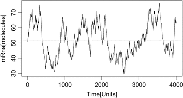

  

  Simulation of the amount of mRNA by Gillepsie (Exercise 5.11) with parameters κ = 1. 08, γ ₀ = 1. 0, β ₁ = 10, γ ₁ = 0. 1

  Fig. 5.52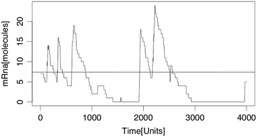

  

  Simulation of the amount of mRNA by Gillepsie (Exercise 5.11) with parameters κ = 0. 08, γ ₀ = 1. 0, β ₁ = 10, γ ₁ = 0. 1

5.12

Let x denote the number of transcribed proteins.

Submodel “binding of promotor region”:

rate non-bound promotor region to bound promotor region: κ x ⁿ

rate bound promotor region to non-bound promotor region: γ

Let p denote the probability to be bound,

$$\displaystyle{\dot{p} =\kappa x^{n}(1 - p) -\gamma p}$$

i.e. the quasi-steady state reads

$$\displaystyle{p = \frac{\kappa x^{n}} {\kappa x^{n}+\gamma } = \frac{x^{n}} {x^{n} +\gamma /\kappa }}$$

i.e. $x_{0} = (\gamma /\kappa )^{1/n}$.

The R-program reads:

# define rate constants (part (a))

kap  = 0.01;   # binding to the promotor region

gam0 = 1;     # average time units promotor bound: 1

bet1 = 10;    # transcription rate if promotor region

bound

bet0 = 0.1;   # transcription rate if promotor region

not bound

gam1 = 1;     # average time span of one mRNA

molecule

nn   = 5;     # Hill Coefficient

# time step

dt = 0.05;   # length of time steps

# state of the system

state = c(0,0)  # promotor bound (0/1), no mRNA

oneStep <- function(){

   # one time step: mRNA only

   newState = state;    # copy the state

   # change promotor reagion

   if (newState[1]==1){

      # dissoziation

      if (runif(1)< dt*gam0){

         newState[1] = 0;

      }

   } else {

      # assotiation

      if (runif(1)< dt*kap*state[2]**nn){

         newState[1] = 1;

      }

   }

   # handle no of mRNA:

   # transcription

   if (runif(1)< dt*((bet1-bet0)*state[1]+bet0)){

      newState[2] = newState[2] + 1;

   }

   # degradation

   if (runif(1)< dt*state[2]*gam1){

      newState[2] = newState[2] - 1;

   }

   state <<- newState;

}

# run

set.seed(1234);

state = c(0, 6);   # high maount of mRNA

#state = c(0, 1);    # low amount of mRNA

res = state;

for (i in 1:4000) {

   oneStep();

   res <- rbind(res, state);

   plot(res[,2], type = "l", xlab="Time[Units]",

                        ylab = "mRna[molecules]");

}

The result fo the simulation is shown in Fig. 5.53. The bistable behaviour of the ODE-model can be found back in the strong dependency on the initial condition. Though the theory about Markov processes tells us, that there is one unique, invariant measure, and any simulation eventually samples from, this measure, the Markov chain does not mix very well. Realisations tend to stay either at low mRNA levels (between 0 and 2), or at high levels (around 10). Only very seldom, random effects will cause the chain from one of the two regions into the other. This effect is well investigated, see e.g. the considerations about the double-wells potential in [77].

Fig. 5.53

Simulation of the amount of mRNA by Gillepsie (Exercise 5.12). The time course strongly depends on the initial value. Parameters κ = 0. 01, γ = 1, β ₁ = 10, β ₀ = 0. 1, γ ₁ = 1, and n = 5

5.13 A positive feedback consists of a signal that enhances its own production in a synergistic way. This synergism happens e.g. by polymerization.

Consequently, we define the locations as S ₁, S ₂, where S ₁ denote the monomers, and S ₂ the dimers. The transitions T ₁ describes the production of monomers, the transition T ₂ the dimerization, T ₃ the dissotiation of dimeres, and T ₄ the degradation of monomers (we again assume that dimers are stable and are not degraded).

• (a) The edges and their weight are

  Edge	Weight
  $(T_{1},S_{1})$	1
  $(S_{2},T_{1})$	L
  $(T_{1},S_{2})$	L
  $(S_{1},T_{4})$	1
  $(S_{1},T_{2})$	2
  $(T_{2},S_{2})$	1
  $(S_{2},T_{3})$	1
  $(T_{3},S_{1})$	2

  Let K > 1 be the capacity for both locations S ₁ and S ₂.

Remark: the transition T ₁ takes L dimers and delivers at the same time L dimers. This ensures that T ₁ can be only active if there are enough dimers.

• (b) Conflicting transitions are (in case that M(S ₁) = 2) T ₂ and T ₄.

Resolution: We could implement a mechanism that ensures that only one of both transition is active (like mentioned in the lecture), or we could switch to a rate-controlled Petri-net (where each transition only takes place at time points, distributed according to a regular Poisson process). We take the latter choice (as this is more natural for the biological system we aim at).

• (c) We determine the incidence matrix, in determining the transition vectors for all transitions:

  $$\displaystyle\begin{array}{rcl} t(T_{1})& =& \left (\begin{array}{c} 1\\ 0\end{array} \right ) {}\\ t(T_{2})& =& \left (\begin{array}{c} - 2\\ 1\end{array} \right ) {}\\ t(T_{3})& =& \left (\begin{array}{c} 2\\ -1\end{array} \right ) {}\\ t(T_{4})& =& \left (\begin{array}{c} - 1\\ 0\end{array} \right ){}\\ \end{array}$$

  Thus,

  $$\displaystyle{I = \left (\begin{array}{cccc} 1& - 2&2& 0\\ 0 & - 2 &2 & -1\end{array} \right )..}$$

S-Invariants:

We determine y s.t. y ^T I = 0 As the rank of the matrix I is two, y = 0 is the only solution. There is no mass conservation at all in the system.

T-Invariants:

We determine q s.t. Iq = 0. Again, as we know the rank of I is two, we expect a two-dimensional space of solutions, spanned by e.g.

$$\displaystyle{(0,1,10)^{T},(-2,0,1,2)^{T}.}$$

The first vector tells us that simultaneously firing of T ₂ and T ₃ does not change the state. The second vector has necessarily a negative entry (this negative entry cannot removed by adding multiples of the first vector etc.; either the first of the last entry is always negative) and thus there are no further combinations of transitions that leave the state invariant.

5.14 Let

$$\displaystyle\begin{array}{rcl} f(u,v)& =& (a - u + u^{2}v)\gamma {}\\ g(u,v)& =& (b - u^{2}v)\gamma. {}\\ \end{array}$$

For computing the stationary states of the diffusionless system we get:

$$\displaystyle\begin{array}{rcl} f(u,v) = 0\quad \Leftrightarrow \quad v = -\frac{a} {u^{2}} + \frac{1} {u}& & {}\\ g(u,v) = 0\quad \Leftrightarrow \quad v = \frac{b} {u^{2}},& & {}\\ \end{array}$$

taken together − a + u = b, i.e., u = a + b and $v = \frac{b} {(a+b)^{2}}$.

As all coordinates are positive if the parameters are chosen positive (as usual), no further restrictions concerning parameter values for guaranteeing positivity.

The general Jacobian matrix reads

$$\displaystyle{J = \left (\begin{array}{cc} -\gamma +2\gamma uv& \gamma u^{2} \\ - 2\gamma uv & -\gamma u^{2} \end{array} \right ).}$$

Inserting the stationary state coordinates:

$$\displaystyle{J =\gamma \left (\begin{array}{cc} - 1 + 2 \frac{b} {a+b} & (a + b)^{2} \\ - 2 \frac{b} {a+b} & - (a - b)^{2} \end{array} \right )}$$

With Proposition 5.39, the conditions for the desired behaviour are

$$\displaystyle\begin{array}{rcl} -1 + 2 \frac{b} {a + b}&>& 0 {}\\ -(a + b)^{2}& <& 0 {}\\ -1 + 2 \frac{b} {a + b} - (a + b)^{2}& <& 0 {}\\ (a + b)^{3}&>& 0 {}\\ \end{array}$$

(the second and the forth condition are satisfied anyway)

5.15

• (a) The stationary equations read

  $$\displaystyle\begin{array}{rcl} 0& =& D\varDelta u {}\\ -D\frac{d} {d\nu }u(x)\vert _{\vert x\vert =R}& =& d_{1}u(x)\vert _{\vert x\vert =R} - d_{2}v {}\\ 0& =& -kv +\int _{\vert x\vert =R}d_{1}u(x)\,do - 4\pi R^{2}\,d_{ 2}v {}\\ \end{array}$$

  and $\lim _{\vert x\vert \rightarrow \infty }u(x) = u_{0}$. As the cell is a ball, we expect a radial symmetric solution. The Laplace operator in this setting yields an ODE, (r = | x | )

  $$\displaystyle{u^{{\prime\prime}} + \frac{2} {r}u^{{\prime}} = 0}$$

  i.e.

  $$\displaystyle{u^{{\prime}}(r) =\tilde{ C}_{ 0}e^{-2\ln (r)} =\tilde{ C}_{ 0}r^{-2}}$$

  and

  $$\displaystyle{u(r) = C_{1} + \frac{C_{0}} {r}.}$$

  As $\lim _{\vert x\vert \rightarrow \infty }u(x) = u_{0}$, we immediately find C ₁ = u ₀.

  We now turn to the boundary condition. As ν is the outer normal, we have

  $$\displaystyle{\frac{\partial } {\partial \nu }u(x)\vert _{\vert x\vert =R} = -u^{{\prime}}(R) = \frac{C_{0}} {R^{2}}}$$

  and hence the boundary condition reads

  $$\displaystyle{\frac{-DC_{0}} {R^{2}} = d_{1}(u_{0} + C_{0}/R) - d_{2}v}$$

  and the equation for the internal oxygen dynamics yields

  $$\displaystyle{0 = -kv + 4\pi R^{2}(u_{ 0} + C_{0}/R)d_{1} - 4\pi R^{2}\,v\,d_{ 2}.}$$

  All in all, we find a linear system of equations for (C ₀, v),

  $$\displaystyle\begin{array}{rcl} \left (\begin{array}{cc} D + d_{1}\,R& - d_{2}\,R^{2} \\ 4\pi Rd_{1} & - (k + 4\pi R^{2}\,d_{2})\end{array} \right )\left (\begin{array}{c} C_{0} \\ v\end{array} \right ) = \left (\begin{array}{c} - R^{2}\,d_{1}u_{0} \\ - 4\pi R^{2}d_{1}u_{0}\end{array} \right )& & {}\\ \end{array}$$

  i.e.

  $$\displaystyle\begin{array}{rcl} \left (\begin{array}{c} C_{0}\\ v\end{array} \right )& =& \frac{\left (\begin{array}{cc} - (k + 4\pi R^{2}d_{ 1})& d_{2}\,R^{2} \\ - 4\pi Rd_{2} & D + d_{1}R\end{array} \right )\left (\begin{array}{c} - R^{2}\,d_{ 1}u_{0} \\ - 4\pi R^{2}d_{1}u_{0}\end{array} \right )} {-(D + d_{1}R)(k + 4\pi R^{2}d_{2}) + 4\pi d_{1}d_{2}R^{3}} {}\\ & =& \frac{1} {-D(k + 4\pi R^{2}d_{2}) - d_{1}kR}\left (\begin{array}{cc} - (k + 4\pi R^{2}d_{ 1})& d_{2}\,R^{2} \\ - 4\pi Rd_{2} & D + d_{1}R\end{array} \right ) {}\\ & & \times \left (\begin{array}{c} - R^{2}\,d_{ 1}u_{0} \\ - 4\pi R^{2}d_{1}u_{0}\end{array} \right ) {}\\ & & {}\\ \end{array}$$

  From that, we find

  $$\displaystyle{C_{0} = \frac{-kR^{2}d_{1}u_{0} + 4\pi R^{4}d_{1}(d_{1} - d_{2})u_{0}} {-D(k + 4\pi R^{2}d_{2}) - d_{1}kR} }$$

  and

  $$\displaystyle\begin{array}{rcl} v& =& v(R) = \frac{4\pi R^{3}d_{1}d_{2}u_{0} - 4\pi R^{2}d_{1}u_{0}(D + d_{1}R)} {D(k + 4\pi R^{2}d_{2}) + d_{1}kR} {}\\ & =& \frac{-4\pi Dd_{1}u_{0}R^{2}} {D(k + 4\pi R^{2}d_{2}) + d_{1}kR} = \frac{4\pi Dd_{1}u_{0}R} {D(k + 4\pi Rd_{2}) + d_{1}k} {}\\ \end{array}$$

• (b) We find at once that

  $$\displaystyle{v(R) \rightarrow 0\qquad \text{ for }R \rightarrow 0}$$

  in a monotonously way (note that x ²∕(a + bx + cx ²) has a positive derivative for a, b, c > 0 and x > 0) i.e. the cell size should be small in order to minimize the oxygen content within the cell. The reason is, that the cell minimizes its surface in this way, and thus no oxygen is able to penetrate the cell. However, it is not really a good idea to minimize the cell surface: also nutrient etc. will not come in by diffusive processes, and a lot of energy is needed to establish active pumps that increase (for nutrient) the rate d ₂ proportional to 1∕R.

References

L. Arnold, Random Dynamical Systems (Springer, Berlin/New York, 2003)
M. Barbarossa, C. Kuttler, A. Fekete, M. Rothballer, A delay model for quorum sensing of Pseudomonas putida. BioSystems 102, 148–156 (2010)
A. Becskei, L. Serrano, Engineering stability in gene networks by autoregulation. Nature 405, 590–593 (2000)
H. Bisswanger, Enzyme Kinetics: Principles and Methods (Wiley-VCH, Weinheim, 2008)
H. De Jong, Modeling and simulation of genetic regulatory systems: a literature review. J. Comput. Biol. 9, 67–103 (2002)
O. Diekmann, S.A. van Gils, S.M.V. Lunel, H.O. Walther, Delay Equations (Springer, New York, 1995)
R. Driver, Ordinary and Delay Differential Equations (Springer, New York/Heidelberg/ Berlin, 1977)
L. Edelstein-Keshet. Mathematical Models in Biology (SIAM, Philadelphia, 2005)
S. Ellner, J. Guckenheimer, Dynamic Models in Biology (Princeton University Press, Princeton, 2006)
M. Elowitz, S. Leibler, A synthetic oscillatory network of transcriptional regulators. Nature 403, 335–338 (2000)
M. Englmann, A. Fekete, C. Kuttler, M. Frommberger, X. Li, I. Gebefügi, P. Schmitt-Kopplin, The hydrolysis of unsubstituted N-acylhomoserine lactones to their homoserine metabolites; Analytical approaches using ultra performance liquid chromatography. J. Chromotogr. 1160, 184–193 (2007)
A. Fekete, C. Kuttler, M. Rothaller, B. Hense, D. Fischer, K. Buddrus-Schiemann, M. Lucio, J. Müller, P. Schmitt-Kopplin, A. Hartmann, Dynamic regulation of N-acyl-homoserine lactone production and degradation in Pseudomonas putida IsoF. FEMS Microbiol. Ecol. 72, 22–34 (2010)
R. Field, E. Körös, R. Noyes, Oscillations in chemical systems, part 2. Thorough analysis of temporal oscillations in the bromate-cerium-malonic acid system. J. Am. Chem. Soc. 94, 8649–8664 (1972)
C. Gardiner, Handbook of Stochastic Methods (Springer, Berlin/New York, 1983)
T.S. Gardner, C.E. Cantor, J.J. Collins, Construction of a genetic toggle switch in Escherichia coli. Nature 403, 339–403 (2000)
A. Gierer, H. Meinhard, A theory of biological pattern formation. Kybernetik 12, 30–39 (1972)
T. Gillespie, A general method for numerically simulating the stochastic time evolution of coupled chemical reactions. J. Comput. Phys. 22, 403–434 (1976)
A. Goldbeter, D.E. Koshland, An amplified sensitivity arising from covalent modification in biological systems. Proc. Natl. Acad. Sci. USA 78, 6840–6844 (1981)
M. Golubitsky, D. Schaeffer, Singularities and Groups in Bifurcation Theory (Springer, New York, 1985)
J.-L. Gouzé, Positive and negative circuits in dynamical systems. J. Biol. Syst. 6, 11–15 (1998)
K.P. Hadeler, D. Glas, Quasimonotone systems and convergence to equilibrium in a population genetic model. J. Math. Anal. Appl. 95, 297–303 (1983)
B. Hense, C. Kuttler, J. Müller, M. Rothballer, A. Hartmann, J. Kreft, Does efficiency sensing unify diffusion and quorum sensing? Nat. Rev. Microbiol. 5, 230–239 (2007)
S. Hooshangi, R. Weiss, The effect of negative feedback on noise propagation in transcriptional gene networks. Chaos 16, 026108 (2006)
F.J. Isaacs, J. Hasty, C.R. Cantor, J.J. Collins, Prediction and measurement of an autoregulatory genetic module. Proc. Natl. Acad. Sci. 100, 7714–7719 (2003)
D. Jones, M. Plank, B. Sleeman, Differential Equations and Mathematical Biology (CRC, Boca Raton, 2010)
H. Kaplan, E. Greenberg, Diffusion of autoinducers is involved in regulation of the Vibrio fischeri luminescence system. J. Bacteriol. 163, 1210–1214 (1985)
S. Kauffman, Metabolic stability and epigenesis in randomly constructed genetic nets. J. Theor. Biol. 22, 437–467 (1969)
M. Krupa, P. Szmolyan, Relaxation oscillation and canard explosion. J. Differ. Equ. 174, 312–368 (2001)
C. Kuttler, B. Hense, Finetuning for the mathematical modelling of quorum sensing regulation systems. Int. J. Biomath. Biostat. 1, 151–168 (2010)
T. Lipniacki, P. Paszek, A. Mariciniak-Czochra, A. Basier, M. Kimmel, Transcriptional stochasticity in gene expression. J. Theor. Biol. 238, 348 (2006)
J. Maybee, J. Quirk, Qualitative problems in matrix theory. SIAM Rev. 11, 30–51 (1969)
J. Müller, C. Kuttler, B. Hense, M. Rothballer, A. Hartmann, Cell-cell communication by quorum sensing and dimension-reduction. J. Math. Biol. 53, 672–702 (2006)
J. Müller, C. Kuttler, B. Hense, S. Zeiser, V. Liebscher, Transcription, intercellular variability and correlated random walk. Math. Biosci. 216, 30–39 (2008)
J. Müller, H. Uecker, Approximating the dynamics of communicating cells in a diffusive medium by ODEs – homogenization with localization. J. Math. Biol. 65, 1359–1385 (2012)
J. Murray, Mathematical Biology II: Spatial Models and Biomedical Applications (Springer, New York, 2003)
W.-L. Ng, B.L. Bassler, Bacterial quorum-sensing network architectures. Ann. Rev. Genet. 43, 197–222 (2009)
M. Renardy, R.C. Rogers, An Introduction to Partial Differential Equations (Springer, New York, 1992)
N. Rosenfeld, J.W. Young, U. Alon, P.S. Swain, M.B. Elowitz, Genetic regulation at the single-cell level. Science 307, 1962–1965 (2005)
H. Smith, Monotone Dynamical Systems: An Introduction to the Theory of Competitive and Cooperative Systems (AMS, Providence, 1995)
H. Smith, An Introduction to Delay Differential Equations with Applications to the Life Sciences. (Springer, New York, 2011)
H.L. Smith, Periodic orbits of competitive and cooperative systems. J. Differ. Equ. 65(3), 361–373 (1986)
E.H. Snoussi, Necessary conditions for multistationarity and stable periodicity. J. Biol. Syst. 6, 3–9 (1998)
S. Swift, J.P. Throup, P. Williams, G.P.C. Salmond, G.S.A.B. Stewart, Quorum sensing: a population–density component in the determination of bacterial phenotype. Trends Biochem. Sci. 21, 214–219 (1996)
R. Thom, Structural Stability and Morphogenesis (W.A. Benjamin, Reading, 1980)
T. Tian, K.Burage, Stochastic models for regulatory networks of the genetic toggle switch. Proc. Natl. Acad. Sci. 103, 8372–8377 (2006)
A. Turing, The chemical basis of morphogenesis. Philos. Trans. R. Soc. Lond. B 237, 37–72 (1952)
J. Tyson, The Belousov-Zhabotinskii Reaction. Lecture Notes in Biomathematics (Springer, Berlin, 1976)
M. Wieser, Atomic weights of the elements. Pure Appl. Chem. 78, 2051–2066 (2006)
P. Williams, K. Winzer, W.C. Chan, M. Cámara, Look who’s talking: communication and quorum sensing in the bacterial world. Philos. Trans. R. Soc. B 362, 1119–1134 (2007)
A. Winfree, The prehistory of the Belousov-Zhabotinsky oscillator. J. Chem. Educ. 61, 661–663 (1984)
Author information
Authors and Affiliations