
Abstract
Near-infrared reflectance (NIR) spectroscopy is a technique that shows many possibilities in the field of testing chemical and physical properties of soil. This paper is aimed to design a prototype of an integrated optoelectronic sensing system capable of estimating soil macronutrients- Nitrogen (N), Phosphorus (P), Potassium (K), pH and Organic Carbon (OC) which play major role in the process of plant growth. 24 soil samples have been collected from farming fields of Birbhum, West Bengal and calibrated using near infrared reflectance spectroscopy. Partial least square (PLS) model along with Standard Normal Variate (SNV) pre-treatment technique has been developed to extract features from the spectroscopic plot which is required for development of field deployable system. The handheld interface attempted in this paper comprises of a simple soil sieve, the output of which is fed in the optoelectronic system which exposes the sieved soil sample to selected IR wavelengths and processes the photodiode output using ARDUINO microcontroller. The trained PLS model embedded in the microcontroller provides estimation of the essential macronutrients with appreciable accuracy. This indigenous system is expected to enhance the scope of precision agriculture in rural India.
1 Introduction
Soil whose main role is to provide nutrients in the process of plant growth [1], is the foundation of agriculture. Soil nutrients affect various aspects like stomatal control, root growth stimulation, growth of leaves and fruits. Fertilizers have traditionally been used throughout the history of agriculture to fulfil the nutrient requirement of soil thereby increasing the crop yield. But, the ever increasing prices of fertilizer and growing ecological concern over chemical run-off into source of drinking water has brought the issue of soil nutrient analysis, precision agriculture and site specific management to the fore-front. Hence, its testing will be ensuring: optimal use of fertilizer, environment protection, optimization of the crop yield, product quality enhancement, increase in yield and precision agriculture. The main objective of this project is to realize an integrated sensing system capable of detecting major soil macronutrients (N, P, K, pH and OC) which are indicators of soil fertility.
1.1 NIR Spectroscopy for Precision Agriculture
The conventional laboratory soil testing techniques are quite complex, time consuming, and expensive for large sample density and hence several alternative methods have been researched [2]. Amongst them, spectroscopy has been used explored extensively and since it is non-invasive, rapid and chemical free. Taking into account the advantages of NIR (750–2500 nm) over other regions of electromagnetic spectrum and also the response of several primary molecules with direct correlation (N, OC, moisture) and certain secondary molecules with indirect correlation (K, pH, P, Ca, Mg, clay content), in the past 15 years, NIR spectroscopy has gained wide acceptance due to its most salient feature which is its ability to record spectra for solid and liquid samples in situ, without any sample preparation. It is an analytical technique that characterizes material on the basis of spectral properties resulting from weak overtones and combination of fundamental vibrations due to stretching and bending of N−H, C−O, C−H bonds [2].
1.2 Data Analysis
Along with capability of soil NIR-spectra to give information about presence of several components, they are largely non-specific, quite weak and broad due to overlapping of absorption of soil constituents and their often small concentrations in soil. Therefore, the information present in spectra needs to be mathematically extracted from the spectra so that they can be correlated with soil properties we are interested in. Hence, the analysis of soil diffusion reflectance spectra requires the use of che- mometric techniques and multivariate calibration [3]. A number of multivariate techniques (PLSR, partial component regression (PCR), step-wise multiple linear regression (SMLR), boosted tree (BT), regression forest (RF)) were compared by Vasques [4] based on the mean R2 (coefficient of determination) and mean RMSE which showed predictive ability of the techniques decreased in the following order: PLSR > SMLR > BT > PCR > RF. Shi [5] compared SMLR, PLSR and SVMR for estimating total nitrogen(TN) with visible/NIR spectroscopy using the effect of first and second derivative which concluded that PLSR along with derivative pre-processing technique was the most suitable regression method for soil TN content estimation. The goal of study conducted by He [6] was to analyze the potential of NIR spectroscopy with PLSR as calibration technique for estimation of N, P, K, OM and pH which showed that NIRS was a technique that could be considered to have good potential for assessing soil N, OM and pH with regression coefficients of 0.93, 0.93, 0.91 respectively. On the basis of existing reports, it is observed that PLSR outperforms all the other multivariate calibration technique in order to relate spectral data to the reference data obtained by laboratory techniques. The PLS algorithm was created as a way of assessing the structural relationships among blocks of variables. It will extract spectral factors over wide range of wavelength, simultaneously relating it with analyte concentration [7]. PLSR as calibration along with SNV as pre-treatment technique have been used in his paper to establish the calibration model. There has not been much work to implement the PLSR model in hardware.
1.3 Field Deployable NIR Based Sensing System
There are some commercially available non-destructive sensor probes based on principles of electromagnetic induction, frequency/time dependent reflectance and ground penetrating radar with varying range of target nutrients and high accuracy of measurement but they are too expensive to be affordable by a farmer [8]. Moreover, the in-built software needs to be recalibrated for local soils to obtain reasonable estimation of nutrients and this flexibility is not present in most of the products. Thus, the proposed design in the paper targets at developing an indigenous field deployable NIR spectroscopic system with optimized hardware components and software with minimal complexity to enable the realization of a simple and cost effective instrument. In this paper, soil samples have been collected from various locations of Birb- hum, West Bengal and have been tested by standard chemical methods in an agriculture laboratory. These results have been correlated with NIR spectroscopic output and the trained coefficients of the PLSR model have been developed. This trained model has then been embedded in a microcontroller and interfaced with the optimized optical system.
2 Materials and Methods
2.1 Soil Sampling and Laboratory Testing
A total of 24 soil samples have been collected in 2 sampling events conducted by Loka Kalyan Parishad, in various test fields across Birbhum District, West Bengal, India. Typical description of each includes crop, exact location and respectable farmer’s name as given in Table 1.
12 soil samples have been divided into 2 groups:
-
(i)
Group A: Sent to Soil Testing Laboratory, Rathindra Krishi Vigyan Kendra, Visva Bharti, Sriniketan, West Bengal for testing of N, P, K, pH and OC by conventional laboratory techniques and the results obtained is shown in Table 2.
Table 2 Laboratory test report -
(ii)
Group B: 12 Samples have been used for spectral data acquisition. The remaining 12 samples have been used for testing and validation of developed model.
2.2 Spectroscopy
Group B samples have been dried and sieved (<2 mm), and then kept in air tight containers. As NIR spectral data is drastically affected by water content in the sample under consideration, so any further interference with moisture in the atmosphere has been avoided by preserving them in Vacuum Desiccator. Spectral measurements have been carried out using the setup as shown in Fig. 1.

Experimental setup for spectra measurement
Setup in Fig. 1 comprises of NIR Spectrometer: DWARF-Star (range-900–1700 nm, resolution-3 nm), light Source: Tungsten Lamp of 5000 Watt-hours and software: Spectrawiz. 5 spectra have been recorded for each of the 12 samples and mean spectra has been obtained by averaging. A typical mean Reflectance spectra for all the samples (superimposed) obtained using UnscramblerX tool shown in Fig. 2.

Mean reflectance spectra
2.3 Pre-processing and Establishment of Calibration Model
We obtained the spectral response at 502 different wavelengths (in 879–1755.75 nm range), but wavelengths beyond 879–1700 nm range does not contain much information, so noise cut has been performed, thereby producing analysis range at 458 different wavelengths for noise-free calibration model development for each of the macro-nutrient to be estimated. After noise cut, the spectral data has been imported to UnscramblerX (version 10.4, CAMO Software) for developing a regression model so as to estimate the best regression, pre-processing combination that will provide optimal estimation of response matrix. Factors are basically the linear combination of variables (i.e. wavelength) that we have in the raw spectra which are used to construct PLS regression model. It follows a basic thumb rule, given by Eq. 1:
In order to cut down the time for algorithm development along with the processing, we preferred UnscramblerX for finding out the optimal number of factors that can be used for the best estimation for the components of our interest using PLSR Model.
The score plots in Fig. 3 shows that pre-treatment of data has enabled the spectral information to express more variability in N concentration. Initially 99% of spectral data contained in 2 factors expressed 42% of N concentration variability while in case of pre-treated data, using 77% of spectral data we can express 41% of N concentration variation. Similar results have been obtained for the remaining Y variables (P, K, pH and OC).

a Score plot with raw data. b Score plot with pre-treated data
3 Algorithm Realization in Microcontroller
The basis for the algorithm development can be outlined as:
-
PLS Model aims to find factors (linear combination of X variables i.e. wavelengths) that best explains the results corresponding to Y variables by an ordinary least square regression.
-
Built using NIPALS (non-iterative partial least squares) algorithm, which splits the data matrix (spectral: X as well as response: Y matrix) into score matrix.
3.1 Data Reduction and Preparation
X matrix initially after noise cut (by eliminating out of range frequencies) was still containing 458 spectral information for each soil sample and we had 12 such samples. Taking into consideration that hard-wiring of such a huge amount of data (12 × 458) will require large memory in microcontroller which we will be using for hardware implementation of algorithm, we have followed manual variable elimination technique so as to reduce the spectral data to make it practical and easily realisable. We omitted spectral data at every third wavelength starting from that available at 900 nm. This led to reduction of order of spectral matrix to 12 × 304. Optimal pre-treatment technique (SNV transform) has been selected after comparative study of the available techniques (derivative, MSC, SNV etc.) in order to deal with non-homogenous distribution of particles in sample that arises due to:
-
Particle size difference
-
Sample density variation
-
Sample morphology difference
-
Spectral variations due to intermolecular hydrogen bonds (moisture content variability).
Also, various quantities of response matrix have been measured in different scaling (kg/ha, unit less, %), hence they have also been auto-scaled (mean centred followed by scaling with standard deviation) and X1 and Y1 have been obtained.
3.2 Algorithm
For each factor to be calculated the following steps have to be followed:
-
Take tstart = largest column of X1
and ustart = largest column of Y1.
-
w′ = u′/x/u′u.
\( w^{\prime}_{\text{new}} = w^{\prime}_{{{\text{old}}^{\prime } }} ||w^{\prime}_{\text{old}} ||\;({\text{normalization}}) \).
t = X1 w/w′w.
q′ = t′Y1/t′t.
\( q^{\prime}_{\text{new}} = q^{\prime}_{{{\text{old}}^{\prime } }} ||q^{\prime}_{\text{old}} ||\;({\text{normalization}}) \).
u = Yq/q′/q.
Check convergence of t by Eq. 2
$$ err = norm\left( {initial \, t - new \, t} \right)/norm\left( {new \, t} \right) $$(2)If err > tolerance limit go to second step.
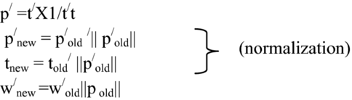
p′, q′, w′, t and u are saved for prediction and estimation step.
b = t′X1/t′t.
-
Calculation of residuals from Eqs. 3 and 4:
$$ X1_{new} = X1_{old} - tp $$(3)$$ Y1_{new} = Y1_{old} - btq^{\prime} $$(4)

From here go to the first step for next factor.
3.3 Estimation
Once the regression model has been built for every input spectra of test sample, then estimation reduces to 3 steps as shown below:
-
testd = IN1w
-
IN1new = IN1old − testdp′
-
OP1 = E b testdq′
- | ||:
-
Euclidean norm
- X:
-
Spectral matrix (12 × 304)
- Y:
-
Response matrix (12 × 5)
- X1:
-
pre-processed Spectral matrix (12 × 304)
- Y1:
-
auto-scaled Response matrix (12 × 5)
- t:
-
column vector of scores for X (12 × 1)
- p′ :
-
row vector of loadings for X (1 × 304)
- w′ :
-
row vector of weights for X ( 1 × 304)
- u:
-
column vector of scores for Y (12 × 1)
- q′ :
-
row vector of loadings for Y (1 × 5)
- b:
-
regression coefficient
- t:
-
estimated score for input IN to produce output OP
Here summation has been performed over two factors. Each of the regression steps have been performed in Arduino version 1.8.5 (used as compiler) using Arduino board (preferred because of huge memory availability). The pictorial view of the microcontroller model is shown in Fig. 4.

Pictorial view of the microcontroller model
4 Implementation of the Hardware
The complete hardware of the system comprises of the optoelectronic components, driver circuit for LEDs and photodiode, Arduino due board and the interface for soil placement. To integrate the optoelectronic components with the microcontroller, the following observations have been made:
-
Spectral Response at 960 nm is sensitive to N, P, pH, OC.
-
Spectral Response at 1450 nm is sensitive to N, P, K, OC.
Inclusion of spectral information at 1100, 1200 and 1300 nm will enhance accuracy of estimation of N, P, pH as well as OC [6].
On the basis of intensive study of market availability, LEDs with peak wavelengths—970, 1070, 1200,1300 and 1450 nm (Marubeni Optoelectronics, USA) have been used for illumination and InGaAs photodiode of 5 mm active diameter (GPD Optoelectronics, USA) has been selected to sense the reflectance. The same microcontroller which has the embedded software will also select the desired wavelengths sequentially and store the photodiode output for each wavelength. The scheme is shown in Fig. 5. As we have decided to use 5 LEDs of various peak wavelengths (with LEDs placed at 120), the photodiode has been placed in the center as shown in Fig. 6.in circular arrangement, such that percentage of light reflected by sample in case of each LED remains same [9].

Schematic diagram

Arrangement of LED and photo diode
Entire optical setup was covered from the sides with black box and a glass plate acting as interface for soil measurement (Fig. 7).

a Top view of monitoring system. b Sensing system in working mode
First of all the developed system was calibrated with the spectral data of soil samples with the developed optical arrangement. Following are the steps for soil nutrient estimation with the developed system is as follows:
-
i.
Provide the supply voltage through adapter
-
ii.
Put the disposable cup inverted on the glass plate covering the effective area of photodiode, take the blank reading for calibration purpose.
-
iii.
Take ~30 g of soil in the disposable cup ad invert it as in the calibration step.
-
iv.
As the LCD Screen displays “press key” message. Press the key.
-
v.
LCD Screen will start showing N(kg/ha), P(kg/ha), K(kg/ha), pH, OC(%) respectively each for the duration of 5 s.
As mentioned in step iii we have taken 25–30 g of soil sample Table 3 compares the volume of soil sample used by the developed monitoring system with that required in conventional technique [10]:
From the above table we can infer that comparatively less amount of soil sample is required when the proposed design is used for soil testing.
Depending on the moisture content of the soil, the response might vary for similar concentration of the other components and hence local calibration might be required [11, 12]. To incorporate this effect, we have provision in our software to select and update the required training data set, by measuring the moisture separately with a commercially available meter. Similar techniques of local calibration and provision to combat with moisture variability have been adopted by other researchers [13, 14]. Further, soil moisture has very strong absorption at 1459 and 1950 nm, so these wavelengths have been completely avoided while designing the proposed system. Moreover, variation in moisture content is much severe at surface level than beneath the soil surface, so in our training and testing, soil sample below the surface has been used.
5 Results and Discussion
A typical test result is indicated in Table 4.
From the above observation we conclude that NIRS combined with PLSR can provide fair estimation for N (error: 2.03%) followed by that for OC (error: 5.21%), pH (error: 8.67%), P and K (error: 12.2% and 15.42% respectively).
A comparison of our developed soil measurement unit with the existing reflectance based hand held sensors is given in Table 5.
It is observed from Table 5 that the proposed software in the measuring system is capable of estimating all the five constituents of the soil i.e. N, P, K, pH and OC together which are not available in the existing hand held meters. Further, the RMSE value of the constituent is also comparable to the previous reports. With extensive field testing of this system, it is expected to enhance the scope of precision agriculture in rural India through on-site testing of soil macronutrients.
References
Toth B, Mako A, Gergely TO (2014) Role of soil properties in water retention characteristics of main Hungarian soil types. J Cent Eur Agric 15:137–153
Joseph V (2010) Sinfield, Daniel Fagerman, Oliver Colic, Evaluation of sensing technologies for on-the-go detection of macro-nutrients in cultivated soils. Comput Electron Agric 70(1):1–18
Martens H, Naes T (1989) Multivariate calibration. Wiley, Chichester, p 419
Vasques GM, Grunwald S, Sickman JO (2008) Comparison of multivariate methods for inferential modeling of soil carbon using visible/near-infrared spectra. Geoderma 146:14–25
Shi T, Cui L, Wang J, Fei T, Chen Y, Wu G (2012) Comparison of multivariate methods for estimating soil total nitrogen with visible/near-infrared spectroscopy. Springer Science Business Media B.V., pp 363–375
He Yong, Huang Min, Garc’ia Annia, Hern’andez Antihus, Song Haiyan (2007) Prediction of soil macronutrients content using near-infrared spectroscopy. Comput Electron Agric 58:144–153
Dale (2012) Chemometrics tools for NIRS and NIR HSI Review I. Bull UASMV Cluj Agric 69(1):70–76
Mohapatra AG, Lenka SK (2015) Sensor system technology for soil parameter sensing in precision agriculture: a review. J Agric Phys 15(2):181–202
Treiman AH, Shelfer TD (2000) Manually portable reflectance spectrometer, US Patent 6043893A, pp 1–10
Westerman RL, Baird JV, Christensen NW, Fixen PE, Whitney DA (1990) Soil-testing and plant analysis, 3 edn. Soil Science Society of America Book Series, pp 73–228
Adamchuk VI, Hummel JW, Morgan MT, Upadhyaya SK (2004) On-the-go soil sensors for precision agriculture. Comput Electron Agric 44:71–91
Shibusawa S, Sato H, Hirako S, Otomo A, Sasao A (2000) A revised soil spectrophotometer. In: Proceedings of 2nd IFAC/CIGR international workshop on biorobotics II, pp 225–230
Liu W, Upadahyaya SK, Kataoka T, Shibusawa S (1996) Development of a texture/soil compaction sensor. In: Proceedings of the Third International Conference on Precision Agriculture. ASA-CSSA-SSSA, pp 617–630
An X, Li M, Zheng L, Liu Y, Sun H (2014) A portable soil nitrogen detector based on NIRS. Precis Agric 15:3–16. Springer Science Business Media, New York, pp 3–16
Lee WS, Bogrekci I (2007) Portable raman sensor for soil nutrient detection, US Patent 2007/0013908 A1, pp 1–12
Holland KH (2013) Optical real-time soil sensor, US Patent 8,451,449 B2, pp 1–18
Stone ML, Needham D, Solie JB, Raun WR, Johnson GV (2005) Optical spectral reflectance sensor and controller, US. Patent, pp 1–16
Acknowledgements
We would like to acknowledge Prof. Rajib Bandyopadhyay and Mr. Somdeb Chanda, Department of Instrumentation and Electronics of Jadavpur University for extending their support in conducting the NIR measurements for calibration. We are grateful to Prof. S. Bhaumik of IIEST Shibpur, who is heading the rural technology project in the Institute for providing the necessary financial assistance.
Author information
Authors and Affiliations
Corresponding author
Editor information
Editors and Affiliations
Rights and permissions
Copyright information
© 2019 Springer Nature Singapore Pte Ltd.
About this paper

Cite this paper
Sharma, P., Samanta, N., Gan, S., Bhattacharyya, D., RoyChauduri, C. (2019). A Cost Effective and Field Deployable System for Soil Macronutrient Analysis Based on Near-Infrared Reflectance Spectroscopy. In: Saha, S., Ravi, M. (eds) Rural Technology Development and Delivery. Design Science and Innovation. Springer, Singapore. https://doi.org/10.1007/978-981-13-6435-8_23
Download citation
DOI: https://doi.org/10.1007/978-981-13-6435-8_23
Published:
Publisher Name: Springer, Singapore
Print ISBN: 978-981-13-6434-1
Online ISBN: 978-981-13-6435-8
eBook Packages: EngineeringEngineering (R0)