
Abstract
The Hopf bifurcation theorem provides an effective criterion for finding periodic solutions for ordinary differential equations. Although various proofs of this classical theorem are known, there seems to be no easy way to arrive at the goal.
Access this chapter
Tax calculation will be finalised at checkout
Purchases are for personal use only
Notes
- 1.
- 2.
- 3.
In the case of f(λ ∗, 0), in particular, f(λ ∗, x) = f(λ ∗, x) − f(λ ∗, 0) = D x f(λ ∗, 0)x + φ(λ ∗, x). Thus, φ(λ ∗, x) is a residue term of the linear approximation of f(λ ∗, x).
- 4.
See Maruyama [12], pp. 281–283 for the implicit function theorem in infinite dimensional spaces.
- 5.
Let \(\mathfrak {L}(\mathfrak {X}, \mathfrak {Y})\) be the space of bounded linear operators of \(\mathfrak {X}\) into \(\mathfrak {Y}\). M and N are bounded linear operators of \(\mathbb {R}\) into \(\mathfrak {L}(\mathfrak {X}, \mathfrak {Y})\). Hence each of M and N can be regarded as a point of \(\mathfrak {L}(\mathfrak {X}, \mathfrak {Y})\). Mv ∗ and Nv ∗ are points of \(\mathfrak {Y}\). Thus we can let P act on them.
- 6.
cf. Lemma 10.5 on p. 15.
- 7.
Related topics are discussed in Ambrosetti- Prodi [1] pp. 17–21.
- 8.
Let \(\mathfrak {V}\) and \(\mathfrak {W}\) be a couple of Banach spaces. Assume that a function φ of an open subset U of \(\mathfrak {V}\) into \(\mathfrak {W}\) is Gâteaux-differentiable in a neighborhood V of x ∈ U. We denote by δφ(v) the Gâteaux-derivative of φ at v. If the function \(v \mapsto \delta \varphi (v)(V\rightarrow \mathfrak {L}(\mathfrak {V}, \mathfrak {W}))\) is continuous, then φ is Fréchet-differentiable. cf. Maruyama [12] pp. 236–237.
- 9.
- 10.
This is a special case of the Rellich– Kondrachov Compactness Theorem. Evans [5] pp. 272–274.
- 11.
If a 2π-periodic function \(\varphi : \mathbb {R}\rightarrow \mathbb {R}\) is absolutely continuous and its derivative φ′ belongs to \(\mathfrak {L}^2([0,2\pi ], \mathbb {R})\), then the Fourier series of φ uniformly converges to φ on \(\mathbb {R}\). The k-th Fourier coefficient of φ′ is given by \(ik\hat {\varphi }(k)\), where \(\hat {\varphi }(k)\) is the k-th Fourier coefficient of φ.
- 12.
span{ξ} denotes the subspace of \(\mathbb {C}^n\) spanned by ξ.
- 13.
Set \(\mu p(t)+\nu q(t) =\mu (\gamma \cos t -\delta \sin t)+\nu (\gamma \sin t+\delta \cos t) = (\mu \gamma +\nu \delta )\cos t+(\nu \gamma -\mu \delta )\sin t=0.\) Then we have
$$\displaystyle \begin{aligned} \begin{cases} \mu \gamma +\nu \delta =0,\\ \nu \gamma -\mu \delta =0. \end{cases} \end{aligned}$$It follows that
$$\displaystyle \begin{aligned} \begin{cases} \mu \nu \gamma +\nu ^2\delta =0,\\ \mu \nu \gamma -\mu ^2\delta =0. \end{cases} \end{aligned}$$Hence (ν 2 + μ 2)δ = 0. If μ ≠ 0 or ν ≠ 0, δ must be zero. And so ξ = γ, that is \(\xi =\bar {\xi }\) (real vector). Thus we get a contradiction.
- 14.
Let \(f : \mathbb {R}\rightarrow \mathbb {R}\) (we may replace \(\mathbb {R}\) by \(\mathbb {R}^n\)) be a 2π-periodic function which is integrable on [− π.π]. Furthermore, we assume \(\hat {f}(0)=0\) (\(\hat {f}(0)\) is the Fourier coefficient corresponding to k = 0). If we define
$$\displaystyle \begin{aligned} F(t)=f(0)+\int_0^t f(\tau )d\tau, \end{aligned}$$F is a 2π-periodic continuous function and
$$\displaystyle \begin{aligned} \hat{F}(k)=\frac{1}{ik}\hat{f}(k), \quad k\neq0. \end{aligned}$$ - 15.
For any \((\alpha _0, \beta _0)\in \mathbb {C}^n\times \mathbb {C}\), there exist some \(\lambda _0\in \mathbb {C}\) and \(\gamma _0\in (i\omega ^*I-A_{\mu ^*})(\mathbb {C}^n)\) such that α 0 = λ 0 ξ + γ 0. Such λ 0 and γ 0 are unique. Let (α 0, β 0) = (0, 0). Then we must have λ 0 = 0 and γ 0 = 0. The equation
$$\displaystyle \begin{aligned} \begin{pmatrix} (i\omega ^*I-A_{\mu ^*})\theta \\ \langle \eta, \theta \rangle \end{pmatrix} = \begin{pmatrix} 0\\ 0 \end{pmatrix} \end{aligned}$$has a unique solution \(\theta =0 (\in \mathbb {C}^n)\) because Ker\([i\omega ^*I-A_{\mu ^*}]\cap \mathrm {Ker} \langle \eta, \cdot \rangle =\mathrm {Ker} [i\omega ^*I-A_{\mu ^*}]\cap [i\omega ^*I-A_{\mu ^*}](\mathbb {C}^n)=\{ 0\}\). Thus we conclude that D (λ,θ) g(μ ∗, iω ∗, 0) is injective.
- 16.
iω ∗ is a simple eigenvalue, again by Assumption 2.
- 17.
Look at Fig. 11.2. For the sake of an intuitive exposition, the vectors η, ξ and κ are treated as real vectors. By \(\langle \eta, \xi \rangle =\parallel \eta \parallel \cdot \parallel \xi \parallel \cos \theta =1\), it follows that \(\parallel \eta \parallel =1/\parallel \xi \parallel \cos \theta \). Hence
$$\displaystyle \begin{aligned} \varPi (\kappa )=\xi \langle \eta, \kappa \rangle =(\parallel \kappa \parallel \cos \zeta /\parallel \xi \parallel \cos \theta )\cdot \xi . \end{aligned}$$Fig. 11.2 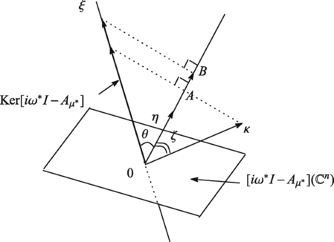
Spectral projection
Since \(\parallel \kappa \parallel \cos \zeta =0A\) (the length of the segment) and \(\parallel \xi \parallel \cos \theta =0B\),
$$\displaystyle \begin{aligned} \varPi (\kappa )=\frac{0A}{0B}\cdot \xi . \end{aligned}$$Here ζ is the angle between η and κ, and θ is the one between ξ and η. κ can be represented uniquely as κ = αη + βz for some \(\alpha ,\beta \in \mathbb {C}\) and \(z\in [i\omega ^*I-A_{\mu ^*}](\mathbb {C}^n)\). On the other hand, η can be represented uniquely in the form η = aξ + bz′ for some \(a,b\in \mathbb {C}\) and \(z'\in [i\omega ^*I-A_{\mu ^*}](\mathbb {C}^n)\). Since ∥ η ∥2 = 〈aξ + bz′, η〉 = a〈ξ, η〉 + b〈z′, η〉 = a, it follows that η =∥ η ∥2 ξ + bz′. Hence we have
$$\displaystyle \begin{aligned} \kappa =\alpha \eta +\beta z=\alpha \parallel \eta \parallel ^2\xi +(\alpha bz'+\beta z). \end{aligned}$$Furthermore, Π(κ) = 〈η, κ〉ξ = 〈η, α ∥ η ∥2 ξ + (αbz′ + βz)〉ξ = α ∥ η ∥2 ξ. (〈η, αbz′ + βz〉 = 0 because \(\alpha bz'+\beta z\in [i\omega ^*I-A_{\mu ^*}](\mathbb {C}^n).\) ) Thus we obtain
$$\displaystyle \begin{aligned} \kappa =\varPi (\kappa )+(\alpha bz'+\beta z). \end{aligned}$$This is the direct sum of \(\mathbb {C}^n \) corresponding to span{ξ} and \([i\omega ^*I-A_{\mu ^* }](\mathbb {C}^n)\).
- 18.
Express each of the Fourier coefficients of y by the direct sum corresponding to span{ξ} and \([i\omega ^*I-A_{\mu ^*}](\mathbb {C}^n)\), and delete all the terms which do not contribute to the former.
- 19.
\(\dot {x}\) and \(\ddot {x}\) denote the first and second derivatives of x with respect to t, respectively.
- 20.
See Theorem 3.6 (p. 13).
- 21.
Assume that \(\varphi _n:[a, b] \rightarrow \mathbb {R}\) is of class \(\mathfrak {C}^1 \;(n=1, 2, \cdots )\) and \(S(t)=\displaystyle {\sum _{n=1}^\infty } \varphi _n(t)\) is convergent. If \(\displaystyle {\sum _{n=1}^\infty } \varphi ^{\prime }_n(t)\) converges uniformly, S(t) is differentiable and \(S^{\prime }(t)=\displaystyle {\sum _{n=1}^\infty } \varphi _n^{\prime }(t)\). cf. Takagi [21], pp. 158–159, Stromberg [20] pp. 214–215. We assumed \(r \geqq 3\) to use this theorem.
- 22.
See footnote 11 on p. 15.
- 23.
For an introductory exposition of business cycle theory, see Maruyama [15], Chap. 18.
- 24.
We obtain s = −ε(μ + δ) + f′(0). It follows from this relation and (11.61) that
$$\displaystyle \begin{aligned} \varepsilon = s(\mu + \delta) - \delta f'(0) = s(\mu + \delta) - \delta(s + \varepsilon(\mu + \delta)), \end{aligned}$$which gives
$$\displaystyle \begin{aligned} \mu^* = \frac{\varepsilon}{s-\delta\varepsilon}(\delta^2+1). \end{aligned}$$ - 25.
See Yamaguti [22], p. 25.

References
Ambrosetti, A., Prodi, G.: A Primer of Nonlinear Analysis. Cambridge University Press, Cambridge (1993)
Carleson, L.: On the convergence and growth of partial sums of Fourier series. Acta Math. 116, 135–157 (1966)
Chang, W.W., Smyth, D.J.: The existence and persistence of cycles in a non-linear model of Kaldor’s 1940 model re-examined. Rev. Econ. Stud. 38, 37–44 (1971)
Crandall, M.G., Rabinowitz, P.H.: The Hopf bifurcation theorem. MRC Technical Summary Report, No. 1604, University of Wisconsin Math. Research Center (1976)
Evans, L.: Partial Differential Equations. American Mathematical Society, Providence (1998)
Frisch, R.: Propagation problems and inpulse problems in dynamic economics. In: Economic Essays in Honor of Gustav Cassel. Allen and Unwin, London (1933)
Hicks, J.R.: A Contribution to the Theory of the Trade Cycle. Oxford University Press, London (1950)
Hopf, E.: Abzweigung einer periodishcen Lösung von einer stationären Lösung eines Differentialsystems. Ber. Math. Phys. Sächsische Akademie der Wissenschafters, Leipzig 94, 1–22 (1942)
Hunt, R.A.: On the convergence of Fourier series. In: Proceedings of the Conference on Orthogonal Expanisions and their Continuous Analogues, Southern Illinois University Press, Carbondale, pp. 234–255 (1968)
Kaldor, N.: A model of the trade cycle. Econ. J. 50, 78–92 (1940)
Keynes, J.M.: The General Theory of Employment, Interest and Money. Macmillan, London (1936)
Maruyama, T.: Suri-keizaigaku no Hoho (Methods in Mathematical Economics). Sobunsha, Tokyo (1995) (Originally published in Japanese)
Maruyama, T.: Existence of periodic solutions for Kaldorian business fluctuations. Contemp. Math. 514, 189–197 (2010)
Maruyama, T.: On the Fourier analysis approach to the Hopf bifurcation theorem. Adv. Math. Econ. 15, 41–65 (2011)
Maruyama, T.: Shinko Keizai Genron (Principles of Economics). Iwanami Shoten, Tokyo (2013) (Originally published in Japanese)
Masuda, K. (ed.): Ohyo-kaiseki Handbook (Handbook of Applied Analysis). Springer, Tokyo (2010) (Originally published in Japanese)
Samuelson, P.A.: Interaction between the multiplier analysis and the principle of acceleration. Rev. Econ. Stud. 21, 75–78 (1939)
Samuelson, P.A.: A synthesis of the principle of acceleration and the multiplier. J. Polit. Econ. 47, 786–797 (1939)
Shinasi, G.J.: A nonlinear dynamic model of short run fluctuations. Rev. Econ. Stud. 48, 649–656 (1981)
Stromberg, K.R.: An Introduction to Classical Real Analysis. American Mathematical Society, Providence (1981)
Takagi, T.: Kaiseki Gairon (Treatise on Analysis), 3rd edn. Iwanami Shoten, Tokyo (1961) (Originally published in Japanese)
Yamaguti, M: Hisenkei Gensho no Sugaku (Mathematics of Nonlinear Phenomena). Asakura Shoten, Tokyo (1972) (Originally published in Japanese)
Yasui, T.: Jireishindo to Keiki Junkan. In:Kinko-bunseki no Kihon Mondai. (Self-oscillations and trade cycles. In: Fundamental Problems in Equilibrium Analysis.) Iwanami Shoten, Tokyo (1965) (Originally published in Japanese)
Author information
Authors and Affiliations
Rights and permissions
Copyright information
© 2018 Springer Nature Singapore Pte Ltd.
About this chapter

Cite this chapter
Maruyama, T. (2018). Hopf Bifurcation Theorem. In: Fourier Analysis of Economic Phenomena. Monographs in Mathematical Economics, vol 2. Springer, Singapore. https://doi.org/10.1007/978-981-13-2730-8_11
Download citation
DOI: https://doi.org/10.1007/978-981-13-2730-8_11
Published:
Publisher Name: Springer, Singapore
Print ISBN: 978-981-13-2729-2
Online ISBN: 978-981-13-2730-8
eBook Packages: Mathematics and StatisticsMathematics and Statistics (R0)