
Abstract
Random sequences play the key role in network security applications. Randomness testing schemes are very important to ensure the randomness qualities for relevant sequences. This chapter proposes a visual scheme based on variant construction to measure sequences to intuitively show some combinatorial properties of key stream generated by stream ciphers. Basic models are described. This scheme provides a flexible framework for the variant measure method on the key stream of stream ciphers to describe randomness in various combinatorial maps.
You have full access to this open access chapter, Download chapter PDF
Keywords
1 Introduction
Random numbers play an important role in many network protocols and encryption schemas on various network security applications [1], for example, visual crypto, digital signatures, authentication protocols and stream ciphers. To determine whether a random sequence is suitable for a cryptographic application, the NIST has published a series of statistical tests as standards.
In network security applications, the stream ciphers play a key role that have faster throughput and easier to implement compared to block ciphers [2]. RC4, the famous stream cipher, is suitable for large packets in Wireless LANs [3]. It has been used for encrypting the internet traffic in network protocols such as Sockets Layer (SSL), Transport Layer Security (TLS), Wi-Fi Protected Access (WPA), etc. [2].
eSTREAM project collected stream ciphers from international cryptology society [4] to promote the design of efficient and compact stream ciphers suitable for widespread adoptions. After a series of tests, algorithms submitted to eSTREAM are selected into two profiles. One is more suitable for software and another one is more suitable for hardware. Non-linear structures and recursive are playing the essential roles in new development.
Different visual schemes are required to test randomness of random sequences on different stream ciphers. Along this direction, this chapter proposes a flexible framework to handle a set of mete measurements on different combinatorial projections.
2 Variant Combinatorial Visualization
Architecture of variant visualization is shown in Fig. 1.

Visualization architecture
The variant visualization architecture is separated into four core components: EAC, SCC CC and VC.
-
RGC Randomness Generate Component generate a random sequence;
-
VSC Variant Statistic Component handles the statistic process using the variant measure method [5];
-
CC Combinatorial Component chooses combinations;
-
VC Visualization Component makes visualization based on SCC measures and CC vectors.
The input n is the length of the binary sequence. The stream ciphers could be changed to any stream cipher that can generate binary sequence. This section focuses on the variant measure module and the visual method module.
A visual example of RC4 will be described in Sect. 2.5.
2.1 Variant Logic Framework
The variant logic framework has been proposed in [6]. Li [7] used the variant measure method to generate different symmetry results [5] based on cellular automata schemes [8]. Under such construction, even some random sequences show symmetry properties in distributions.
Under variant construction, the variant conversion operator can be defined as follows:
It is convenient to list relevant variant logic variables shown in Table 1.
In the variant measure method, each sequence is converting from binary sequence to probability which generated by counting the number of each variable in \( \left\{ { \bot , + , - ,{ \top }} \right\} \) and computes the probability of each variable. The measurement method is shown in Table 1.
The variant measure method provides a set of results in measures of different 0–1 sequences. The following mechanism can transfer stream cipher sequences as relevant measures.
The essential models of variant scheme are described as follows.
2.2 VSC Variant Statistic Component
The VSC component converts the binary sequence to variant sequence in VCM module, and to compute probabilities and entropies in PECM module, respectively. The component is shown in Fig. 2.

Variant statistic component
VCM Variant Conversion Module
VCM module transfers input binary sequences by following steps:
-
Step 1.
Generate an n bit binary sequence \( S = S_{1} S_{2} S_{3} \ldots S_{n} \) by a stream cipher.
-
Step 2.
Shift X to left by M bit (M is the length of shifting) and generate a new binary sequence \( S^{\prime } = S_{1}^{\prime } S_{2}^{\prime } S_{3}^{\prime } \ldots S_{n - M}^{\prime } = S_{1 + M} S_{2 + M} \ldots S_{n} \).
-
Step 3.
Convert two sequences: S and S′ to a variant sequence \( V = V_{i} = C\left( {S_{i,} S_{i}^{\prime } } \right),\quad i = 1,2,3 \ldots \left( {n - M} \right) \).
-
Step 4.
Separate V into \( n/N \) parts. N is the length of each part and \( M \le N \le n \) to form a set of variant sequence groups
-
Step 5.
Separate each item in G into \( N/M \) parts to establish a sequence group
PECM Probability and Entropy Computing Module
PECM converts a variant sequences group to separate it into several parts to compute probability and entropies. The equations computing the parameters have been described in Table 1. The main steps are performed as follows:
-
Step 6.
Compute the probability vector \( P = \left\{ {P_{ \bot } ,P_{ + } ,P_{ - } ,P_{{ \top }} } \right\} \) of each part in G′;
-
Step 7.
Calculate the distribute probability vector \( D = \left\{ {D_{ \bot } ,D_{ + } ,D_{ - } ,D_{{ \top }} } \right\} \) of each part in G based on P vector;
-
Step 8.
Evaluate the entropy vector \( \left\{ {E_{ \bot } ,E_{ + } ,E_{ - } ,E_{{ \top }} } \right\} \) from the D vector.
2.3 CC Combinatorial Component
IIn the CC component, it can be separated into two modules. One is SM module to form the vector selecting and another one is VDM module to perform the visualization.
Visual data is a set of E vectors as input for VC. For E vector, choose a projection as a visual vector to compute the visual result from E vectors. So there will be 16 visual results.
Base on the same number of variables in a combination, the combination set can be integrated into 5 parts. i.e. The selected number of variables in the combination is in 0-4.
Let the classification be \( EC = \left\{ {EC_{0} ,EC_{1} ,EC_{2} ,EC_{3} ,EC_{4} } \right\} \). Since the \( EC_{0} \) is empty, it can be ignored. Only four distributions are of concern in Sect. 2.4.
2.4 Visualization Component
According to the variant measure method, in the rectangular axis, let \( E_{ \bot } \) be the positive axis of X, \( E_{{ \top }} \) be the negative axis of X, \( E_{ + } \) the positive axis of Y, \( E_{ - } \) be the negative axis of Y. The axis is shown in Fig. 3.

Visualization axis
For \( EC_{1} = \left\{ {\left\{ {E_{ \bot } } \right\},\left\{ {E_{ + } } \right\},\left\{ {E_{ - } } \right\},\left\{ {E_{{ \top }} } \right\}} \right\} \), points are distributed to the axis.
For \( EC_{2} = \left\{ {\left\{ {E_{ \bot } ,E_{ + } } \right\},\left\{ {E_{ \bot } ,E_{ - } } \right\},\left\{ {E_{ \bot } ,E_{{ \top }} } \right\},\left\{ {E_{ + } ,E_{ - } } \right\},\left\{ {E_{ + } ,E_{{ \top }} } \right\},\left\{ {E_{ - } ,E_{{ \top }} } \right\}} \right\} \), points are distributed in the shadow area in Fig. 4.

Distribution areas of \( EC_{2} \)
For \( EC_{3} = \left\{ {\left\{ {E_{ \bot } ,E_{ + } ,E_{ - } } \right\},\left\{ {E_{ \bot } ,E_{ + } ,E_{{ \top }} } \right\},\left\{ {E_{ \bot } ,E_{ - } ,E_{{ \top }} } \right\},\left\{ {E_{ + } ,E_{ - } ,E_{{ \top }} } \right\}} \right\} \), points are distributed in the area of \( EC_{1} \) and the area of \( EC_{2} \).
For \( EC_{4} = \left\{ {\left\{ {E_{ \bot } ,E_{ + } ,E_{ - } ,E_{{ \top }} } \right\}} \right\} \), points are distributed in Fig. 5.

Distribution areas of \( EC_{4} \)
2.5 Example
An example is given step by step to show how the algorithm runs. In the example, n, N and M are, respectively, assigned to 40, 16 and 8.
-
Step 1.
Input a 35 bit binary sequence, {010100101110101100101101011
1101101010101}
-
Step 2.
Generates \( S^{\prime } \), {11101011001011010111101101010101}.
-
Step 3.
Generates V, \( \{ + { \top } + - + \bot { \top } + - - { \top } \bot { \top } + - { \top } \bot + { \top } + { \top } + - { \top } \bot { \top } - { \top } - + - { \top } \)}.
-
Step 4.
Separate V into a G vector. The G vector is \( \left\{ {\left\{ { + { \top } + - + \bot { \top } + - - { \top } \bot { \top } + - { \top }} \right\},\left\{ { \bot + { \top } + { \top } + - { \top } \bot { \top } - { \top } - + - { \top }} \right\}} \right\} \).
-
Step 5.
Separate the G into the G′ vector. The G′ vector in the example is \( \left\{ {\left\{ { + { \top } + - + \bot { \top } + , - - { \top } \bot { \top } + - { \top }} \right\},\left\{ { \bot + { \top } + { \top } + - { \top }, \bot { \top } - { \top } - + - { \top }} \right\}} \right\} \).
-
Step 6.
Generate probability vector P of each sequence in G′. The P vector of \( \left\{ { + { \top } + - + \bot { \top } + } \right\} \) is \( \left\{ {P_{ \bot } = 0.125,P_{ + } = 0.5,P_{ - } = 0.125,P_{{ \top }} = 0.25} \right\} \).
-
Step 7.
Compute the distribute probability vector D of each sequence in G from P. The D vector of \( \left\{ { + { \top } + - + \bot { \top } + , - - { \top } \bot { \top } + - { \top }} \right\} \) is shown in Fig. 6.
Fig. 6 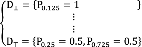
D vectors of \( \left\{ { + { \top } + - + \bot { \top } + , - - { \top } \bot { \top } + - { \top }} \right\} \)

-
Step 8.
Compute the entropy vector E of each sequence in G from D. The E vector of \( \left\{ { + { \top } + - + \bot { \top } + - - { \top } \bot { \top } + - { \top }} \right\} \) is shown in Fig. 7.
Fig. 7 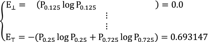
E vectors of \( \left\{ { + { \top } + - + \bot { \top } + - - { \top } \bot { \top } + - { \top }} \right\} \)

-
Step 9.
Compute visual results from E vectors. In the E vectors of \( \left\{ { + { \top } + - + \bot { \top } + - - { \top } \bot { \top } + - { \top }} \right\} \). If the selection is \( \left\{ {E_{ \bot } } \right\} \), points will be \( \left( {0.0,0.0} \right) \). If the selection is \( \left\{ {E_{ \bot } ,E_{{ \top }} } \right\} \), points will be \( \left( {0.0, - 0.693147} \right) \) and \( \left( {0.0,0.0} \right) \). If the selection is \( \left\{ {E_{{ \top }} ,E_{ - } } \right\} \), points will be \( \left\{ {E_{ - } - \left| {E_{{ \top }} } \right|} \right\} = \left( {0.0,0.0} \right) \) and \( \left( {0.0,0.693147} \right) \). If the selection is \( \left\{ {E_{ \bot } ,E_{{ \top }} ,E_{ - } } \right\} \), points will be \( \left\{ {E_{ \bot } ,E_{ - } - \left| {E_{{ \top }} } \right|} \right\} = \left( {0.0,0.0} \right) \) and \( \left( {0.0,0.693147} \right) \).
-
Step 10.
Separate visual results to EC classification. Visual results of the G in the example are shown in Fig. 8.
Fig. 8 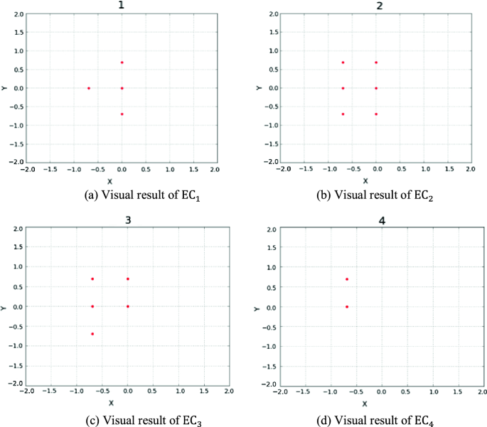
Visual result of the example

3 Result
3.1 Visual Result of RC4
The initial: \( \left\{ {{\mathbf{n}}: 128{,}000,{\mathbf{N}}:128,{\mathbf{M}}:16} \right\} \)
The visual result (Fig. 9).

Visual result of RC4 \( \left\{ {{\mathbf{n}}:128000,{\mathbf{N}}:128,{\mathbf{M}}:16} \right\} \)
The initial: \( \left\{ {{\mathbf{n}}:128{,}000,{\mathbf{N}}:128,{\mathbf{M}}:24} \right\} \)
The visual result (Fig. 10).

Visual result of RC4 \( \left\{ {{\mathbf{n}}:128000,{\mathbf{N}}:128,{\mathbf{M}}:24} \right\} \)
The initial: \( \left\{ {{\mathbf{n}}:128{,}000,{\mathbf{N}}:1000,{\mathbf{M}}:8} \right\} \)
The visual result (Fig. 11).

Visual result of RC4 \( \left\{ {{\mathbf{n}}:128000,{\mathbf{N}}:1000,{\mathbf{M}}:8} \right\} \)
The initial: \( \left\{ {{\mathbf{n}}:100{,}000,{\mathbf{N}}:100,{\mathbf{M}}:24} \right\} \)
The visual result (Fig. 12).

Visual result of RC4 \( \left\{ {{\mathbf{n}}:100000,{\mathbf{N}}:100,{\mathbf{M}}:24} \right\} \)
3.2 Visual Result of HC256
The initial: \( \left\{ {{\mathbf{n}}:128{,}000,{\mathbf{N}}:128,{\mathbf{M}}:16} \right\} \)
The visual result (Fig. 13).

Visual result of HC256 \( \left\{ {{\mathbf{n}}: 128000, {\mathbf{N}}: 128, {\mathbf{M}}: 16} \right\} \)
The initial: \( \left\{ {{\mathbf{n}}:128{,}000,{\mathbf{N}}:128,{\mathbf{M}}:24} \right\} \)
The visual result (Fig. 14).

Visual result of HC256 \( \left\{ {{\mathbf{n}}: 128000, {\mathbf{N}}: 128, {\mathbf{M}}: 24} \right\} \)
The initial: \( \left\{ {{\mathbf{n}}:100{,}000,{\mathbf{N}}:100,{\mathbf{M}}:8} \right\} \)
The visual result (Fig. 15).

Visual result of HC256 \( \left\{ {{\mathbf{n}}: 100000, {\mathbf{N}}: 100, {\mathbf{M}}: 8} \right\} \)
The initial: \( \left\{ {{\mathbf{n}}:100{,}000,{\mathbf{N}}:100,{\mathbf{M}}:16} \right\} \)
The visual result: (Fig. 16).

Visual result of HC256 \( \left\{ {{\mathbf{n}}: 100000, {\mathbf{N}}: 100, {\mathbf{M}}: 16} \right\} \)
4 Conclusion
The visual results show the similar symmetry property of sequences generated by RC4 and HC256. They are showing interesting distributions and can be significantly distinguished from their combinatorial maps. From our models and illustrations, various maps can be integrated by their combinatorial projections to show different spatial distributions on random sequences. Under this configuration, the variant measure method provides a new analysis tool for stream cipher applications in further explorations.
References
S. William, Cryptography and Network Security: Principles and Practice (Pearson Education, 2006)
G. Paul, S. Maitra, RC4 Stream Cipher and Its Variants (CRC Press, 2012)
P. Prasithsangaree, P. Krishnamurthy, Analysis of energy consumption of RC4 and AES algorithms in wireless LANs, in Global Telecommunications Conference, 2003. GLOBECOM ‘03. IEEE, vol. 3, pp. 1445–1449 (2003)
eSTREAM project, http://www.ecrypt.eu.org/stream/
J. Zheng, C. Zheng, T. Kunii, Interactive maps on variant phase spaces- from measurements—micro ensembles to ensemble matrices on statistical mechanics of particle models, in Emerging Applications of Cellular Automata, pp. 113–196, CC BY (2013)
J.Z.J. Zheng, C.H. Zheng, A framework to express variant and invariant functional spaces for binary logic. Front. Electr. Election. 5(2), 163–172 (2010)
Q. Li, Z. Zheng. Spacial distributions for measures of random sequences using 2D conjugate maps, in Proceedings of Asia-Pacific Youth Conference on Communication (APYCC) (2010)
S. Wolfram, Theory and applications of cellular automata. Scientific (1986)
Acknowledgements
This work was supported by the Key Project on Electric Information and Next Generation IT Technology of Yunnan (2018ZI002), NSF of China (61362014) and Yunnan Advanced Overseas Scholar Project.
Author information
Authors and Affiliations
Corresponding author
Editor information
Editors and Affiliations
Rights and permissions
Open Access This chapter is licensed under the terms of the Creative Commons Attribution 4.0 International License (http://creativecommons.org/licenses/by/4.0/), which permits use, sharing, adaptation, distribution and reproduction in any medium or format, as long as you give appropriate credit to the original author(s) and the source, provide a link to the Creative Commons license and indicate if changes were made.
The images or other third party material in this chapter are included in the chapter's Creative Commons license, unless indicated otherwise in a credit line to the material. If material is not included in the chapter's Creative Commons license and your intended use is not permitted by statutory regulation or exceeds the permitted use, you will need to obtain permission directly from the copyright holder.
Copyright information
© 2019 The Author(s)
About this chapter

Cite this chapter
Zheng, J., Wan, J. (2019). Visual Maps of Variant Combinations on Random Sequences. In: Zheng, J. (eds) Variant Construction from Theoretical Foundation to Applications. Springer, Singapore. https://doi.org/10.1007/978-981-13-2282-2_22
Download citation
DOI: https://doi.org/10.1007/978-981-13-2282-2_22
Published:
Publisher Name: Springer, Singapore
Print ISBN: 978-981-13-2281-5
Online ISBN: 978-981-13-2282-2
eBook Packages: EngineeringEngineering (R0)