Microscopic Expressions of Nonlinear Polarization

Abstract

In the SFG processes described in the preceding Chap. 2, material properties were treated as given parameters. This chapter formulates the material properties relevant to the SFG spectroscopy from a microscopic viewpoint. The most important property in the SFG spectra is the frequency-dependent second-order nonlinear susceptibility tensor, χ ⁽²⁾( Ω, ω ₁, ω ₂). We derive χ ⁽²⁾ by the quantum mechanical perturbation theory of light-matter interactions. In the vibrational SFG spectroscopy, vibrational resonance plays a critical role in the nonlinear response of polarization. We further discuss some basic features of χ ⁽²⁾, including the relation of its tensor elements to the light polarizations and molecular orientation.

Appendix

3.1.1 Off-Diagonal Elements of Density Matrix

We have learned in Sect. 3.1 that the density matrix can represent statistical ensemble of states and a pure state in the common formulas. It is instructive to illustrate the distinction between a superposition of quantum states and a statistical ensemble of states. This example is useful to clarify the concept of coherence.

Let us consider two wavefunctions, ϕ ₁ and ϕ ₂, for example. If the two states are superposed in the quantum sense, the state is represented by a wavefunction,

$$\displaystyle \begin{aligned} \psi (t)= c_1 (t) \phi_1 + c_2 (t) \phi_2\ \ \quad\left(\text{ where }\ \left| c_1 (t) \right|{}^2 + \left| c_2 (t) \right|{}^2 = 1\right)\end{aligned} $$

or equivalently by a density matrix

$$\displaystyle \begin{aligned} {{\rho }^{\text{pure}}}(t)=\left( \begin{matrix} {{c}_{1}}c_{1}^{*} & {{c}_{1}}c_{2}^{*} \\ {{c}_{2}}c_{1}^{*} & {{c}_{2}}c_{2}^{*} \\ \end{matrix} \right). {} \end{aligned} $$

(3.57)

The above state in Eq. (3.57) is a pure state, where the probabilities of finding the states ϕ ₁, ϕ ₂ are $P^1 = c_1c_1^*$, $P^2 = c_2c_2^*$, respectively. On the other hand, we consider a statistical ensemble consisting of ϕ ₁ and ϕ ₂ with the probabilities being P ¹ and P ² respectively. This is a mixed state, presented by the following density matrix

$$\displaystyle \begin{aligned} {{\rho }^{\text{mixed}}}(t)={{P}^{1}}\left( \begin{matrix} 1 & 0 \\ 0 & 0 \\ \end{matrix} \right)+{{P}^{2}}\left( \begin{matrix} 0 & 0 \\ 0 & 1 \\ \end{matrix} \right)=\left( \begin{matrix} {{c}_{1}}c_{1}^{*} & 0 \\ 0 & {{c}_{2}}c_{2}^{*} \\ \end{matrix} \right), {} \end{aligned} $$

(3.58)

where $c_1c_1^* = P^1 \; (> 0)$, $c_2c_2^* = P^2 \; (> 0)$. Comparing ρ ^pure and ρ ^mixed, we see that the diagonal elements are common, indicating that the probabilities of finding ϕ ₁, ϕ ₂ are the same. However, the off-diagonal elements are distinct between Eqs. (3.57) and (3.58).

The off-diagonal element $\rho _{12} = \overline {c_1 c_2^*}$ implies correlation between the coefficients (c ₁ and c ₂) of the constituent states (ϕ ₁ and ϕ ₂). To illustrate the physical meaning of off-diagonal elements, we discuss the following two cases that exhibit no off-diagonal elements. Let us consider an ensemble of states {ψ ¹, ψ ², ψ ³, ⋯ }, where each sample ψ ^j is a superposition of two states ($\psi ^j = c_1^j \phi _1 + c_2^j \phi _2$) and has a probability of P ^j in the ensemble.

Case 1. :

First case is an extreme one that ψ ^j is either ϕ ₁ ($c_2^j =0$) or ϕ ₂ ($c_1^j =0$). Then the diagonal element ρ ₁₂ vanishes, $\overline {c_1 c_2^*}=\sum _j P^j c_1^j c_2^{j*}=0$, because either $c_1^j$ or $c_2^j$ is zero in each term of j. This case shows that the off-diagonal element ρ ₁₂ arises from quantum superposition between ϕ ₁ and ϕ ₂.

Case 2. :

The quantum superposition is not a sufficient condition for the off-diagonal elements. We consider another ensemble of $\{ \psi ^j = c_1^j \phi _1 + c_2^j \phi _2 \}$, where the coefficient $c_{m}^{j}=|c_{m}^{j}|\exp (i\theta _{m}^{j})$ (m = 1, 2) has a definite amplitude |c _m| but a random phase factor $\theta _m^j$ (m = 1, 2). Then the ensemble average of the diagonal element has a definite value |c _m|² while the off-diagonal element vanishes, e.g.

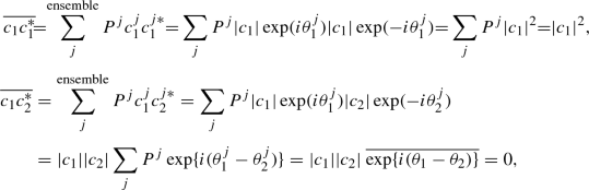
because the average of random phase distribution results in cancellation.

From the two cases, we find that the diagonal element is determined by the square of amplitude |c _m|², irrespective of its phase. On the other hand, the off-diagonal element is sensitive to the relative phase of the two superposition coefficients, c ₁ and c ₂. If the phases of the two coefficients have no correlation, the off-diagonal element disappears via the ensemble average.

In summary, a finite off-diagonal element ρ ₁₂ indicates that there involves a definite quantum superposition between the states ϕ ₁ and ϕ ₂ with some phase relation. In such case the coherence is present between the two states ϕ ₁ and ϕ ₂.

3.1.2 Interaction Energy of Nonmagnetic Materials

In Chap. 3, the perturbation Hamiltonian by the irradiated light is given by H ^′ = −μ ⋅E(t) in Eq. (7.2), which represents the interaction to the electric field E. This is based on the assumption that interaction energy with the magnetic field of light is negligible compared to that with the electric field for ordinary nonmagnetic materials. Here we estimate their relative orders of magnitude to justify this assumption.

The interaction energy of material with the magnetic field H is

$$\displaystyle \begin{aligned} U_m = -m H = - \chi_m H^2, \end{aligned}$$

where m is the magnetization, and χ _m is the magnetic susceptibility, which is dimensionless in the cgs Gauss units. (A possible factor 1/2 is omitted for simplicity to estimate the order of magnitude.) Typical values of χ _m for nonmagnetic materials are in the range of |χ _m| = 10⁻⁴ ∼ 10⁻⁶ for paramagnetic materials, and |χ _m| = 10⁻⁶ ∼ 10⁻⁷ for diamagnetic materials [5]. On the other hand, the interaction energy with the electric field E is analogously presented by

$$\displaystyle \begin{aligned} U_e = - P E = - \chi _e E^2, \end{aligned}$$

where χ _e is the electric susceptibility, also dimensionless in the cgs Gauss units. Typical range of χ _e is in the order |χ _e| = 10⁻¹ ∼ 10⁻². For example, χ _m and χ _e of liquid benzene are roughly estimated to

$$\displaystyle \begin{aligned} \begin{array}{rcl} \chi _m &\displaystyle \simeq &\displaystyle -5.48 \times 10^{-5} \; \mathrm{cm^3/mol} \cdot \frac{0.8765 \; \mathrm{g/cm^3}}{78.11 \; \mathrm{g/mol}} = - 6.1 \times 10^{-7},\\ \chi_e &\displaystyle \simeq &\displaystyle \frac{1}{4\pi } (2.2825 - 1) = 1.0 \times 10^{-1},\end{array} \end{aligned} $$

using the experimental values of molar magnetic susceptibility (− 5.48 × 10⁻⁵ cm³∕mol), density (0.8765 g∕cm³), molecular weight (78.11 g/mol), and dielectric constant (2.2825) [5].

The light field consists of electric and magnetic fields, whose amplitudes are related to |E|≃|H|, as seen in Eq. (2.14). Therefore, the ratio of electric and magnetic interactions U _m∕U _e is evaluated to

$$\displaystyle \begin{aligned} \left| \frac{U_m}{U_e} \right| = \left| \frac{\chi _m H^2}{\chi _e E^2} \right| \simeq \left| \frac{\chi_m}{\chi_e} \right| \ll 1 \end{aligned}$$

This relation confirms that typical interaction energy with magnetic field is much smaller than that with the electric field in ordinary nonmagnetic materials.

3.1.3 Polarizability Approximation for Raman Tensor

This subsection shows that the Raman tensor of Eq. (3.37) is approximated with the polarizability in electronically off-resonant conditions [10, 11, 14]. The Raman tensor defined in Eq. (3.37) includes the states g, n and m, which denote the initial, intermediate and final states, respectively. These states are represented as products of electronic and vibrational states on the basis of the Born-Oppenheimer approximation,

$$\displaystyle \begin{aligned} & \left| g \right\rangle =\left| g^e (\boldsymbol{r},\boldsymbol{R}) \right\rangle \left| g^v (\boldsymbol{R}) \right\rangle , \\ & \left| n \right\rangle =\left| n^e (\boldsymbol{r},\boldsymbol{R}) \right\rangle \left| n^v (\boldsymbol{R}) \right\rangle , \\ & \left| m \right\rangle =\left| m^e (\boldsymbol{r},\boldsymbol{R}) \right\rangle \left| m^v (\boldsymbol{R}) \right\rangle =\left| g^e \right\rangle \left| m^v \right\rangle, {} \end{aligned} $$

(3.59)

where the superscript e designates the electronic states and v the vibrational states. r and R denote the coordinates for electrons and nuclei, respectively. In the ordinary Raman process illustrated in Fig. 3.4, both the initial state g and the final state m are supposed to be the electronically ground state g ^e, while their vibrational states are different. Here we assume that the ground electronic state g ^e is unique and not degenerated. The total energy is also represented as the sum of electronic and vibrational energies,

$$\displaystyle \begin{aligned} & \mathcal{E}_g = \mathcal{E}_g^e + \mathcal{E}_g^v,\\ & \mathcal{E}_n = \mathcal{E}_n^e + \mathcal{E}_n^v, \\ & \mathcal{E}_m = \mathcal{E}_m^e + \mathcal{E}_m^v = \mathcal{E}_g^e + \mathcal{E}_m^v. {} \end{aligned} $$

(3.60)

Fig. 3.4

Raman process in off-resonant condition

We substitute Eqs. (3.59) and (3.60) into the expression of Raman tensor. If the excitation energy ħ Ω is off resonant and thus the condition $\left | \left ( \mathcal {E}_{n}^{e} - \mathcal {E}_{g}^{e} \right )-\hbar \Omega \right | \gg \left | \mathcal {E}_{n}^{v} - \mathcal {E}_{g}^{v} \right |$ is satisfied (see Fig. 3.4), then the denominators of Eq. (3.37) are approximated to be

$$\displaystyle \begin{aligned}\begin{array}{r*{20}l} &\ast \; && \frac{1}{\Omega - \omega _{ng} + i \Gamma _{ng}} &&= {\left[ \Omega -\frac{\left( \mathcal{E}_n^e - \mathcal{E}_g^e \right) + \left( \mathcal{E}_n^v - \mathcal{E}_g^v \right)}{\hbar } + i \Gamma _{ng} \right]}^{-1}\\ &&&&& \cong {\left[ \Omega -\frac{\mathcal{E}_n^e - \mathcal{E}_g^e}{\hbar } + i \Gamma _{ng} \right]}^{-1} =\frac{1}{\Omega -\omega _{ng}^e + i \Gamma _{ng}}, {} \end{array}\end{aligned} $$

(3.61)

$$\displaystyle \begin{aligned}\begin{array}{r*{20}l} &\ast \; &&\frac{1}{\Omega + \omega _{mn} + i \Gamma _{mn}} &&\cong \frac{1}{\Omega + \omega _{nm}^e + i \Gamma _{nm}} = \frac{1}{\Omega + \omega _{ng}^e + i \Gamma _{ng}}. {} \end{array}\end{aligned} $$

(3.62)

Using these approximations of Eqs. (3.61) and (3.62),⁶ the Raman tensor element of Eq. (3.37) is represented by

$$\displaystyle \begin{aligned} & \left\langle g|\alpha _{pq}(\Omega )|m \right\rangle \cong -\sum_{n^e} \sum_{n^v} \left[ \frac{ \left\langle g^v \right|\left\langle g^e | \mu _p | n^e \right\rangle \left| n^v \right\rangle \left\langle n^v \right|\left\langle n^e | \mu _q | m^e \right\rangle \left| m^v \right\rangle }{\Omega -\omega _{ng}^e + i \Gamma _{ng}} \right.\\ & \left. \qquad\qquad\qquad\qquad\qquad-\frac{\left\langle g^v \right| \left\langle g^e | \mu _q | n^e \right\rangle \left| n^v \right\rangle \left\langle n^v \right|\left\langle n^e | \mu _p | m^e \right\rangle \left| m^v \right\rangle }{\Omega +\omega _{ng}^e + i \Gamma _{ng}} \right] \\ & = \left\langle g^v \left| -\sum_{n^e} \left[ \frac{ \left\langle g^e | \mu _p | n^e \right\rangle \left\langle n^e |\mu _q | g^e \right\rangle }{\Omega -\omega _{ng}^e + i \Gamma _{ng}} - \frac{ \left\langle g^e | \mu _q | n^e \right\rangle \left\langle n^e | \mu _p | g^e \right\rangle }{\Omega +\omega _{ng}^e + i \Gamma _{ng}} \right] \right| m^v \right\rangle\\ & =\left\langle g^v (\boldsymbol{R}) | \alpha _{pq} (\Omega ,\boldsymbol{R}) | m^v (\boldsymbol{R}) \right\rangle, {} \end{aligned} $$

(3.63)

where the completeness condition $\sum _{n^v}{\left | n^v \right \rangle \left \langle n^v \right |}=1$ has been adopted. The final expression of α _pq( Ω, R) is no longer an explicit function of the electronic coordinate r, as r is already integrated out in Eq. (3.63). α _pq( Ω, R) means the polarizability of the electronic ground state at the frequency Ω and given nuclear coordinates R. When Ω is far off resonant from the electronic excited state (i.e. $\hbar \Omega \ll \mathcal {E}_n^e - \mathcal {E}_g^e$), the dispersion of α can be neglected and α _pq( Ω, R) is further approximated with the static polarizability, α _pq( Ω, R)≅α _pq( Ω = 0, R).

Bibliography

Boyd RW (2003) Nonlinear optics. Academic, Amsterdam
Dirac PAM (1927) The quantum theory of dispersion. Prof R Soc Lond A114:710–728
Goldstein H, Poole C, Safko J (2001) Classical mechanics, 3rd edn. Pearson, San Francisco
Hayashi M, Lin SH, Raschke MB, Shen YR (2002) A molecular theory for doubly resonant IR-UV-vis sum-frequency generation. J Phys Chem A 106:2271–2282
Haynes WM (ed) (2012) CRC handbook of chemistry and physics, 93rd edn. CRC Press, Boca Raton
Ishiyama T, Morita A (2006) Intermolecular correlation effect in sum frequency generation spectroscopy of electrolyte aqueous solution. Chem Phys Lett 431:78–82
Ishiyama T, Morita A (2007) Molecular dynamics study of gas-liquid aqueous sodium halide interfaces II. analysis of vibrational sum frequency generation spectra. J Phys Chem C 111:738–748
Kramers HA, Heisenberg W (1925) Üder die streuung von strahlung durch atome. Z Phys 31:681–708
Lambert AG, Davies PB, Neivandt DJ (2005) Implementing the theory of sum frequency generation vibrational spectroscopy: a tutorial review. Appl Spec Rev 40:103–145
Long DA (1977) Raman spectroscopy. McGraw-Hill, New York
Long DA (2002) The raman effect. Wiley, New York
Loudon R (2000) The quantum theory of light, 3rd edn. Oxford University Press, Oxford
Mukamel S (1995) Principles of nonlinear optical spectroscopy. Oxford University Press, New York
Placzek G (1934) Rayleigh-streuung und Raman-effekt. Handbuch der Radiologie 6:205–374
Shen YR (1984) The principle of nonlinear optics. Wiley, New York
Weiss PA, Silverstein DW, Jensen L (2014) Non-condon effects on the doubly resonant sum frequency generation of rhodamine 6G. J Phys Chem Lett 5:329–335
Zaleśny R, Bartkowiak W, Champagne B (2003) Ab initio calculations of doubly resonant sum-frequency generation second-order polarizabilities of LiH. Chem Phys Lett 380:549–555
Zheng R-H, Wei W-M, Jing Y-Y, Liu H, Shi Q (2013) Theoretical study of doubly resonant sum-frequency vibrational spectroscopy for 1,1-bi-2-naphthol molecules on water surface. J Phys Chem C 117:11117–11123
Author information
Authors and Affiliations