
Abstract
For pipe flow calculation, the piping system can be divided into two parts, that is single pipe flow and multiple pipes flow. The combination of multiple pipes can make up the pipe network. The researches on orifice and nozzle flow are also meaningful in engineering application. In this chapter, we will first introduce single pipe flow and multiple pipes flow. For multiple pipes flow, we mainly discuss series flow, parallel flow and uniformly variable mass outflow. Then we will figure out characteristics of orifice flow and nozzle flow. For them, we will pay more attention to their discharge coefficients for velocity and flow rate.
5.1 Flow in Single Pipe
Single pipe always involves one pipe with constant diameter. The hydraulic calculation in single pipe is the simplest among pipeline hydraulic calculation, which is a fundamental for the hydraulic calculation in multiple pipes. The flow in single pipe can be classified into short pipe and long pipe flow. For hydraulic calculation in a short pipe, we cannot ignore the minor head loss, otherwise it can be ignored in a long pipe.
5.1.1 Hydraulic Calculation in a Short Pipe
The suction pipe of a pump and siphon all belong to the short pipes, so their minor head loss cannot be neglected in the calculation. The following is an example for short pipe hydraulic calculation.
Example 5.1
As shown in Fig. 5.1, there is a pump installed in a piping system. The diameter of cast iron pipe is \( d = 150\;{\text{mm}}\), and the length is \( l = 180\;{\text{m}}\). The minor loss coefficient of screen filter without bottom valve is \( \zeta_{1} = 6 \), for inlet and outlet of the pipe \( \zeta_{2} = 0.5 \), \( \zeta_{5} = 1 \), for three elbows \( \zeta_{3} = 0.294 \times 3 \), for valve \( \zeta_{4} = 3.9 \). Assuming that the height \( h = 100\;{\text{m}} \), the flow rate \( Q = 225\;{\text{m}}^{ 3} / {\text{h}} \) and the temperature of water \( t = 20\;^{ \circ } {\text{C}} \), find output power of the pump.

A piping system [1]
-
Solution
When \( t = 20\;^{ \circ } {\text{C}} \), the kinematic viscosity of water \( \nu = 1.007 \times \,10^{ - 6} \;{\text{m}}^{ 2} / {\text{s}} \) (Table 1.2), then
Cast iron pipe \( \Delta = 0.30\;{\text{mm}} \), \( \frac{\Delta }{d} = 0.002 \)
Check the Moody chart according to \( \text{Re} \) and \( \Delta /d \), \( \lambda = 0.024 \).
According to the given conditions, \( \sum {\zeta = } \zeta_{1} + \zeta_{2} + \zeta_{3} + \zeta_{4} + \zeta_{5} = 12.28 \), then the equivalent pipe length of minor head loss is
Substituting the equation \( v = \frac{4Q}{{\pi d^{2} }} \) into \( h_{l} = \lambda \frac{{l + \sum {l_{e} } }}{d}\frac{{v^{2} }}{2g} \), we have
Thus, the pump’s head rise is
The output power of the pump is
5.1.2 Hydraulic Calculation in a Long Pipe
We take an example to analyze hydraulic characteristics and calculation method for long pipe flow. As shown in Fig. 5.2, water is drained away from a water tank by a pipe with diameter \( d \), length \( l \) and height \( H \) from water surface to the outlet.

Long pipe flow
With 0–0 as the datum reference, then Bernoulli equation between section 1–1 and 2–2 is:
Because of long pipe, we neglect minor head loss \( h_{r} \) and velocity head \( \frac{{\alpha_{2} v_{2}^{2} }}{2g} \), then we have \( h_{l} = h_{f} \). Assuming that \( v_{1} \approx 0 \), we have
The above equation shows that the total head of long pipe equals frictional loss, and the frictional loss of long pipe flow can be calculated by Chezy formula, namely
where \( Q \) is the flow rate, \( l \) is the length of pipe, and \( K \) is volumetric flow rate which can be referred from textbooks or professional manuals.
The Chezy formula is generally adopted in hydraulic calculation of long pipe flow. \( K \) can be expressed as follows:
The relationship between frictional factor \( \lambda \) and Chezy factor \( c \) can be expressed as follows.
The common empirical formula for Chezy factor \( c \) calculation is Manning formula, that is
where \( R \) is hydraulic radius.
\( n \) is the roughness coefficient which has different values for different types of boundary roughness. In engineering, the approximate values for different \( n \) can be referred from Table 5.1.
\( K \) is the function of \( d \) and \( n \). Table 5.2 gives the values of \( K \) with different \( d \) and \( n \).
Example 5.2
Assuming that the flow rate of a pipe \( Q = 250\;\;{\text{L/s}} \), the length \( l = 2500\;{\text{m}} \), the head \( H = 30\;{\text{m}} \). The material of the pipe is new cast iron. Find the diameter of the pipe.
-
Solution
According to Table 5.2, when \( n = 0.0111 \) and \( K = 2283\;\;{\text{L/s}} \), the diameter of pipe is between 350 and 400 mm, and can be calculated as follows:
5.2 Flow in Multiple Pipes
There are multiple pipes in actual pipe systems. The multiple pipe systems include series flow, parallel flow, variable mass outflow and so on, where only the friction losses are taken into consideration for hydraulic calculation.
5.2.1 Series Flow
As shown in Fig. 5.3, the flow in pipe system which consists of pipes with different diameters is series flow. The flow rate in each pipe may be constant, or variable due to the leakage in the end of each pipe.

Series flow
We assume the length, the diameter, and flow rate of each pipe are \( l_{i} \), \( d_{i} \), and \( Q_{i} \) respectively. The flow rate leakage in each pipe is \( q_{i} \). According to the continuity equation, we have
The relationship between flow rate and head loss of each pipe is
The total head loss of series flow equals to the sum of the head loss in each pipe, that is
If there is no leakage in each pipe, then
Example 5.3
Considering the Example 5.2 with series flow.
-
Solution
Assuming that the length of the pipe with diameter \( d_{1} = 350\;{\text{mm}} \) is \( l_{1} \), so the length of the pipe with diameter \( d_{2} = 400\,\;{\text{mm}} \) is \( l_{2} = l - l_{1} \). Then according to Eq. (5.6), we have
Namely \( 30 = 250^{2} \times \left( {\frac{{l_{1} }}{{1727^{2} }} + \frac{{2500 - l_{1} }}{{2464^{2} }}} \right) \)
So
Therefore, for series flow, the length of the pipe with diameter \( d_{1} = 350\;{\text{mm}} \) is 400 m, and the length of the pipe with diameter \( d_{2} = 400\,\;{\text{mm}} \) is 2500 – 400 = 2100 m.
5.2.2 Parallel Flow
As shown in Fig. 5.4, there are three pipes in parallel between point A and B. The total flow rate is \( Q \). The diameter of each pipe is \( d_{1} \), \( d_{2} \) and \( d_{3} \) respectively, and the length is \( l_{1} \), \( l_{2} \) and \( l_{3} \) respectively. The flow rate of each pipe is \( Q_{1} \), \( Q_{2} \) and \( Q_{3} \) respectively. The head loss is \( h_{f1} \), \( h_{f2} \) and \( h_{f3} \) respectively. The piezometric head difference between point A and B is \( h_{f} \). Because there exists only one piezometric head for each point, the piezometric head difference between point A and B through different pipes is invariable. Thus, the characteristic of parallel flow is that the head loss of each parallel pipe is same.

Parallel flow
So
According to continuity equation, we have
Combing Eq. (5.8) with Eq. (5.9), we can solve many problems about the hydraulic calculation of parallel flow.
Example 5.4
As shown in Fig. 5.4, The diameter of each pipe is \( d_{1} = 150\;{\text{mm}} \), \( d_{2} = 150\;{\text{mm}} \) and \( d_{3} = 200\;{\text{mm}} \) respectively, and the length is \( l_{1} = 500\;{\text{m}} \), \( l_{2} = 350\;{\text{m}} \) and \( l_{3} = 1000\,{\text{m}} \) respectively. The overall flow rate of this parallel piping system is \( Q = 80\;{\text{L/s}} \), and each of these pipes belongs to normal pipe. Find the flow rate of each pipe and the head loss of this parallel piping system.
-
Solution
According to Table 5.2, \( K_{1} = K_{2} = 158.4 \), and \( K_{3} = 341.0 \).
Assuming that the flow rate of pipe 1 is \( Q\,_{1} \), according to Eq. (5.8), the flow rate of pipe 2 is \( Q\,_{2} = Q_{1} \frac{{K_{2} }}{{K_{1} }}\sqrt {\frac{{l_{1} }}{{l_{2} }}} = Q_{1} \times \sqrt {\frac{500}{350}} = 1.195\;Q_{1} \)
The flow rate of pipe 3 is \( Q\,_{3} = Q_{1} \frac{{K_{3} }}{{K_{1} }}\sqrt {\frac{{l_{1} }}{{l_{3} }}} = Q_{1} \times \frac{341.0}{158.4} \times \sqrt {\frac{500}{1000}} = 1.522\,Q_{1} \)
The overall flow rate is \( Q = Q_{1} + Q_{2} + Q_{3} = Q_{1} + 1.195Q_{1} + 1.522Q_{1} = 3.715Q_{1} \)
So
The head loss is \( h_{f} = \frac{{Q_{1}^{2} l_{1} }}{{K_{1}^{2} }} = \frac{{21.5^{2} \times 500}}{{158.4^{2} }} = 9.2\;{\text{m H}}_{ 2} {\text{O}}\, \)
5.2.3 Uniformly Variable Mass Outflow
As shown in Fig. 5.5, assuming that the outlet flow rate is \( Q_{T} \), and the total leakage flow rate is \( Q_{P} \). If the leakage flow rate per unit length along the pipe is same, \( \frac{{Q_{P} }}{l} = q \) is constant. This kind of flow is defined as uniformly variable mass outflow.

Uniformly variable mass outflow [2]
Select arbitrary point M for analysis, and the distance from point M to point A is \( x \). The flow rate in point M is
Then
Integrate above equation, we have
It can approximately equal to
Combining the form of Chezy formula, we rewrite the equation as follows:
where \( Q_{c} = Q_{T} + 0.55Q_{P} \).
When \( Q_{T} = 0 \), Eq. (5.10) can be simplified as
According to Eq. (5.13), the head loss of uniformly variable mass outflow is just a third of the head loss of invariable mass flow with same total flow rate. The reason is that the volumetric flow rate of variable mass outflow decreases gradually along the pipe.
5.2.4 Pipe Network Geometry
The pipe networks for water supply have mainly the following two types of configurations: branched or tree-like configuration (a) and looped configuration (b), as shown in Fig. 5.6.

Pipe networks
A branched network, or a tree network, is a distribution system having no loops. Such a network is commonly utilized for rural water supply. The simplest branched network is a radial network consisting of several distribution mains emerging out from a common input point.
A pipe network in which there are one or more closed loops is called a looped network. Looped networks are preferred from the reliability point of view. If one or more pipelines are closed for repair, water can still reach the consumer by a circuitous route incurring more head loss. This feature is absent in a branched network. With the changing demand pattern, not only the magnitudes of the discharge but also the flow directions change in many links.
5.3 Orifice Flow
Orifice flow refers to fluid outflow from an orifice [3, 4]. When fluid flows out through an orifice into atmosphere, we call this kind of flow as free discharge. When fluid flows out through an orifice into another liquid, we call this kind of flow as submerged discharge.
According to the diameter, orifice can be divided into small orifice and large orifice. Assuming that the head acting on the orifice cross section is H, orifice diameter is d. When \( d < \frac{H}{10} \), the orifice belongs to small orifice; when \( d > \frac{H}{10} \), the orifice belongs to large orifice.
If fluid discharge through an orifice on a container wall might not be affected by sharp edge it has and the thickness of container wall is smaller than 3d, this kind of flow is still supposed to thin-plate orifice flow. Otherwise the discharge of orifice on thick wall of which the thickness is usually bigger than 3d is supposed to nozzle flow, which will be discussed in the next section.
5.3.1 Steady Discharge Through Thin-Plate Orifice
5.3.1.1 Free Discharge of Thin-Plate Orifice
The free discharge through thin-plate orifice is shown in Fig. 5.7. Assuming that the head H is constant, the diameter of the orifice is d and the area is A.

Free discharge of thin-plate orifice
When the fluid enters the orifice, the streamlines cannot change direction sharply due to the inertial effect and they bend gradually along a smooth curvet to converge towards the orifice axis until to a cross section c–c with a roughly distance of 0.5d from inlet.
The cross section c–c is called the vena contracta. Assuming that the area of c–c is Ac, then
where \( \varepsilon \) is contraction coefficient.
Consider the flow between section O–O and c–c in Fig. 5.7. Select a datum reference O′–O′ on the centerline of the orifice, then we write Bernoulli equation between the two sections as
The liquid on cross section c–c is connected with the atmosphere, so we assume Pc = Pa. Since friction loss is very small, only the minor head loss is taken into consideration, that is, \( h_{l} = h_{r} = \zeta \frac{{v_{c}^{2} }}{2g} \), in which \( \zeta \) is minor loss coefficient of orifice. We assume \( \alpha_{0} = \alpha_{c} = 1.0 \), because of the uniform velocity distribution on the orifice. Therefore, the above equation may be transformed into
Then
We express the above equation as follows:
where \( \varphi = \frac{1}{{\sqrt {1 + \zeta } }} \) is discharge coefficient for velocity, and \( H_{0} = H + \frac{{v_{0}^{2} }}{2g} \) is effective head.
Compared with \( v_{c} \), \( v_{0} \) is much smaller and always neglected, so \( v_{c} \) can be approximately expressed as follows.
Thus, according to Eqs. (5.17) and (5.18), the flow rate of orifice flow is
Or
where \( \mu = \varepsilon \varphi \) is discharge coefficient for flow rate.
With different types of orifice and resistance, there will be different values of discharge coefficient. According to many experimental results, the discharge coefficients take values from \( \varphi = 0.97\sim 0.98 \), \( \mu = 0.58\sim 0.62 \).
5.3.1.2 Submerged Discharge
As shown in Fig. 5.8, for submerged discharge, the water jet passing through the orifice will expand rapidly and flow into another liquid.

Submerged discharge
With 0–0 as the datum reference, the Bernoulli equation between section 1–1 and 2–2 is
where, \( h_{l} = h_{r} = \zeta_{s} \frac{{v_{c}^{2} }}{2g} \). \( \zeta_{s} \) is minor loss coefficient of submerged discharge, and it includes two parts: minor loss coefficient of jet contraction \( \zeta \) and minor loss coefficient of jet sudden expansion \( \zeta_{\text{E}} \). We take \( \zeta_{\text{E}} { = }1 \), so \( \zeta_{s} { = }\zeta { + }1 \). We assume \( v_{1} = v_{2} \), \( \alpha_{1} = \alpha_{2} = 1.0 \), \( p_{1} = p_{2} = p_{a} \). Then, Eq. (5.21) can be transformed into
then
where \( H = H_{1} - H_{2} \), which is elevation head difference between upstream and downstream.
Thus, the flow rate of submerged discharge is
where \( \mu \) is discharge coefficient of submerged discharge for flow rate.
Considering that the head of downstream has little influence on the jet contraction and minor loss, we assume the \( \varepsilon \), \( \varphi \), \( \mu \) of submerged discharge are basically the same as free discharge.
Example 5.5
Assuming that there is free discharge of a thin-plate orifice with diameter \( d = 50\,\,{\text{mm}} \), head \( H = 1\,\,{\text{m}} \). Find the flow rate of free discharge. If it is submerged discharge, and the head after the orifice discharge is \( H_{2} = 0.4\;{\text{m}} \), find the corresponding flow rate.
-
Solution
Neglecting the velocity head \( v_{0} \), and taking discharge coefficient for flow rate \( \mu = 0.62 \), according to Eq. (5.20), we have
When it comes to the submerged discharge, the head difference between upstream and downstream is \( Z = H - H_{2} = 1 - 0.4 = 0.6\;{\text{m}} \), then the flow rate is
5.3.2 Discharge Through Big Orifice
As shown in Fig. 5.9, the head in each point on vena contracta is different for big orifice free discharge. In most cases of engineering applications, for big orifice flow rate calculation, we utilize the formula which is similar to small orifice. However, the discharge coefficient for flow rate is determined by the experiments. Thus, the equation to calculate the flow rate is expressed as follows:

Discharge through big orifice
where \( \mu^{{\prime }} \) is discharge coefficient of big orifice for flow rate ranging from \( \mu^{{\prime }} = 0.6\sim 0.9 \).
5.3.3 Unsteady Discharge Through Orifice
Unsteady discharge means that the free surface of the container lowers gradually. We usually pay more attention to the discharge time for unsteady discharge calculation.
As shown in Fig. 5.10, we assume the area of the container cross section is \( A \), the area of orifice is \( a \), the height from free surface of container to orifice is \( y \). During the time \( {\text{d}}t \), the flow rate of orifice discharge can be calculated by Eq. (5.20) shown as follows:

Unsteady discharge through orifice
Assume that the free surface decreases \( {\text{d}}y \) during the time \( {\text{d}}t \). According to the continuity equation, the outflow volume from orifice equals the decreasing volume in the container. We have
Then
The time \( t \) of the free surface decreasing from \( H_{1} \) to \( H_{2} \) is indicated after integrating the above equation as
When \( H_{2} = 0 \), the time of emptying the water in the container is
where \( V \) is the emptying volume of the container, and \( Q_{\hbox{max} } \) is the maximum flow rate at starting time.
Equation (5.25) shows that the emptying time of unsteady discharge is twice the time for same outflow volume in steady discharge with the head \( H_{1} \).
5.4 Nozzle Flow
When a short pipe with length \( l = (3\sim 4)d \) (where \( d \) is the pipe diameter) and same cross section with orifice is connected to the orifice of a container, the outflow in this case is defined as nozzle discharge. The nozzle can be classified into cylindrical outer nozzle (Fig. 5.11a), cylindrical inner nozzle (Fig. 5.11b), conical contracted nozzle (Fig. 5.11c), conical expanding nozzle (Fig. 5.11d), and streamline shape nozzle (Fig. 5.11e).

Different types of nozzle flow
5.4.1 Steady Discharge Through Cylindrical Outer Nozzle
A cylindrical outer nozzle is shown in Fig. 5.12. The water jet passing through the nozzle will contract at first to generate a vena contracta c–c, the distance from inlet is about \( L_{c} = 0.8d \). The vacuum phenomenon occurs as well. Then the jet can fill the nozzle gradually. So only the minor loss would be involved in hydraulic calculation.

Steady discharge through cylindrical outer nozzle
Assuming that the area of nozzle cross section is \( A \). With 0–0 as the datum reference, the Bernoulli equation between section 1–1 and 2–2 is
where \( h_{l} = h_{r} = \sum \zeta \frac{{v^{2} }}{2g} \), \( \sum \zeta \) is the total minor loss coefficient, including the contraction and the expansion of the jet. We take \( \alpha_{1} = \alpha = 1.0 \) and replace \( v_{1} \) with \( v_{0} \). Assuming that \( H_{0} = H + \frac{{v_{0}^{2} }}{2g} \), we have
The velocity can be expressed as
Compared with \( v \), \( v_{0} \) is much smaller and can be neglected, so we have
The flow rate of nozzle discharge is
where \( \varphi \) is discharge coefficient for velocity of cylindrical outer nozzle, \( \mu \) is discharge coefficient for flow rate of cylindrical outer nozzle, and \( \mu = \varphi \). According to the tests, the value of discharge coefficient for flow rate is \( \mu = 0.82 \).
5.4.2 Vacuum Degree of Nozzle
The discharge coefficient for flow rate of orifice is smaller than the one of nozzle due to vacuum generation in the nozzle. The flow rate can be improved a lot after connecting a nozzle on thin-plate orifice.
As shown in Fig. 5.12, when U-tube manometer is connected with the vena contracta c–c, the height of the liquid column in U-tube \( h_{v} \) equals \( 0.75H_{0} \) according to experimental results. The value can also be analyzed by theoretical analysis as follows:
As shown in Fig. 5.12, with 0–0 as the datum reference, the Bernoulli equation between section 1–1 and c–c is
Neglecting \( \frac{{\alpha_{1} v_{1}^{2} }}{2g} \) and assuming that \( \alpha_{c} = 1.0 \), we have
According to the continuity equation, we have
According to Eq. (5.28), we have
Equation (5.30) can be expressed as follows:
Assuming that \( \zeta = 0.06 \) (minor loss coefficient of gradual contraction short pipe in Table 4.10), \( \varepsilon = 0.64 \) and \( \varphi = 0.82 \) usually. Then we have
It can be seen that the bigger \( H_{0} \) is, the higher vacuum will be. The vacuum degree on the vena contracta is 75% of the acting head, which indicates that the function of nozzle is equivalent to increasing the acting head of orifice free discharge by 75%. Therefore, the flow rate of nozzle discharge is much bigger than that of corresponding orifice.
According to the above analysis, the higher vacuum can lead to bigger flow rate. However, in order to ensure the nozzle working normally, the highest vacuum in the nozzle should be restricted. According to the experimental results, the vacuum on the vena contracta should not exceed 7 m H2O, that is
Second, there is restriction on the length of nozzle as well. The most suitable length \( l \) should be about \( 3\sim 4d \).
Example 5.6
As shown in Fig. 5.13, there is a water tank with three cylindrical drainage orifices. The diameter of the drainage orifice is \( d = 0.2\;{\text{m}} \). The thickness of the wall is \( l = 0.7\;{\text{m}} \). The head above the centerline of orifice is \( H = 1.5\;{\text{m}} \). Neglecting the moving velocity \( v_{0} \), find the flow rate of the drainage orifices.

Drainage of a water tank
-
Solution
Since the thickness of the wall \( l = 3.5\,{\text{d}} \), the drainage of this water tank can be regarded as nozzle discharge. Taking discharge coefficient for flow rate \( \mu = 0.82 \), the flow rate of each drainage orifice is
The overall flow rate of these three drainage orifices are
Since the head above the centerline of orifice is \( H = 1.5\;{\text{m}}\,{ < }\, 9\; {\text{m}} \), the discharge of drainage orifice functions normally.
5.4.3 Other Types of Nozzle Discharge
For other types of nozzle discharge, their velocity, and flow rate formulas are the same with that of the cylindrical nozzle. The difference is the discharge coefficient, below are several commonly used nozzles.
5.4.3.1 Streamline Shape Nozzle
As shown in Fig. 5.14a, the discharge coefficient for velocity is \( \varphi = \mu = 0.97 \), and it is suitable for the case of small head loss, big flow rate, and uniform velocity distribution at the outlet.

Common nozzle discharge
5.4.3.2 Conical Expanding Nozzle
As shown in Fig. 5.14b, when \( \theta = 5^{ \circ } \sim 7^{ \circ } \), \( \varphi = \mu = 0.42 \sim 0.50 \). It is suitable for the case of transforming part of kinetic energy to pressure energy, such as the diffuser pipe of ejector.
5.4.3.3 Conical Contracted Nozzle
As shown in Fig. 5.14c, the discharge is dependent on the contraction angle. When \( \theta = 30^{ \circ } 24^{{\prime }} \), \( \varphi = 0.963 \), \( \mu = 0.943 \) is the maximum magnitude. It is suitable for the case of speeding up the ejecting velocity, such as firefighting water gun.
5.5 Problems
-
5.1
As shown in Fig. 5.15, there is a cast iron pipe \( \left( {\Delta = 0.4\;\,{\text{mm}}} \right) \) with constant diameter \( d = 500\;\,{\text{mm}} \), and the length \( l = 100\;\,{\text{m}} \). Water flow belongs to turbulent flow in rough pipes (region V). The minor loss coefficients of inlet and outlet are 0.5 and 1.0 respectively, and for each elbow \( \zeta = 0.3 \). The height from the upstream to the downstream is \( H = 5\;{\text{m}} \). Find the flow rate Q of the pipe.
Fig. 5.15 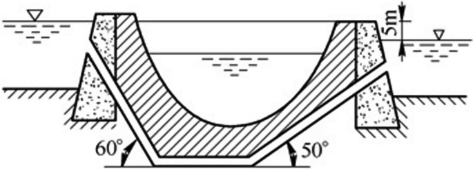
Problem 5.1
-
5.2
The water flows from the high-level reservoir to the low-level reservoir, as shown in Fig. 5.16. Assuming that \( H = 12\;{\text{m}} \). There is a clean steel pipe with the length \( l = 300\;{\text{m}} \) and the diameter \( d = 100\,\,{\text{mm}} \). Find the flow rate of the pipe. If the flow rate \( Q = 150\;\,{\text{m}}^{ 3} / {\text{h}} \), what is the diameter of the pipe?
Fig. 5.16 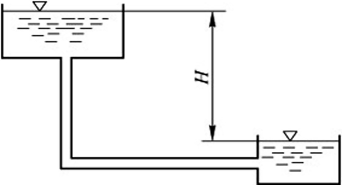
Problem 5.2
-
5.3
As shown in Fig. 5.17, assuming that the total head of this piping system is \( H = 12\;{\text{m}} \), the diameter and length of each pipe is \( d_{1} = 250\,\;{\text{mm}} \), \( l_{1} = 1000\,\;{\text{m}} \), \( d_{2} = 200\,\;{\text{mm}} \), \( l_{2} = 650\,\;{\text{m}} \), \( d_{3} = 150\,\;{\text{mm}} \), \( l_{3} = 750\;{\text{m}} \) respectively. Find the head loss in each pipe, and draw piezometric head line. The pipe is clean with minor head loss neglected.
Fig. 5.17 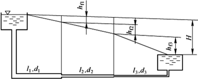
Problem 5.3
-
5.4
As shown in Fig. 5.18, there is a parallel piping system. The flow rate of each pipe is \( Q_{1} = 50\,{\text{L/s}} \), \( Q_{2} = 30\,{\text{L/s}} \) respectively with the length \( l_{1} = 1000\;\,{\text{m}} \), and \( l_{2} = 500\;\,{\text{m}} \). The diameter is \( d_{1} = 200\;\,{\text{mm}} \). The pipe is clean. Find the diameter \( d_{2} \).
Fig. 5.18 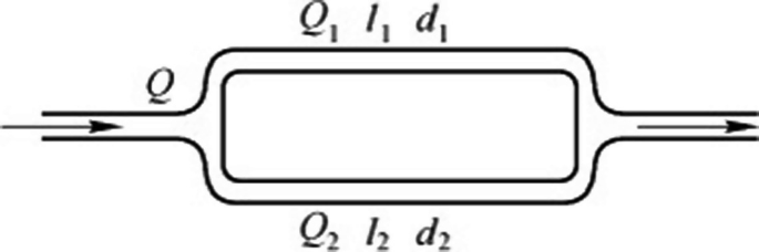
Problem 5.4
-
5.5
As shown in Fig. 5.19, there are three different pipes between B and C. The dimension of each pipe is \( d_{1} = 300\,\;{\text{mm}} \), \( l_{1} = 500\,\;{\text{m}} \), \( d_{2} = 250\,\;{\text{mm}} \), \( l_{2} = 300\,\;{\text{m}} \), \( d_{3} = 400\,\;{\text{mm}} \), \( l_{3} = 800\;{\text{m}} \), \( d_{AB} = 500\,\;{\text{mm}} \), \( l_{AB} = 800\,\;{\text{m}} \), \( d_{CD} = 500\,\;{\text{mm}} \), \( l_{CD} = 400\,\;{\text{m}} \). The pipes all belong to normal pipes. The flow rate in point B is 250 L/s. Find the total head loss in this piping system.
Fig. 5.19 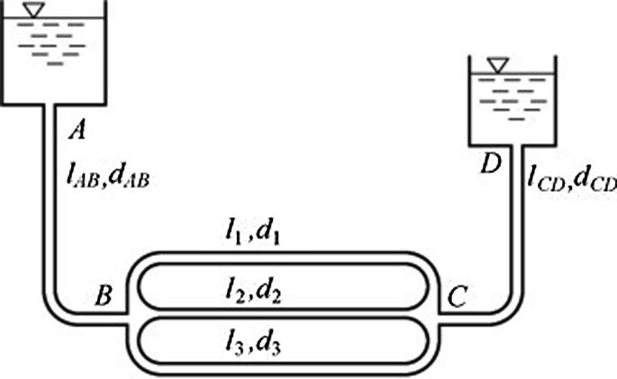
Problem 5.5
-
5.6
The relative pressure on the surface of water tank A is \( p_{0} = 1.313 \times 10^{5} \;{\text{Pa}} \), and water flows from A to B through a series of different pipes, as shown in Fig. 5.20. Assuming that \( H = 8\,\;{\text{m}} \). The dimension of the pipes are \( d_{1} = 200\,\;{\text{mm}} \), \( l_{1} = 200\,\;{\text{m}} \), \( d_{2} = 100\,\;{\text{mm}} \), \( l_{2} = 500\,\;{\text{m}} \) respectively. The pipes all belong to normal pipes. Only the minor head loss from the valve is taken into consideration. Find the flow rate Q of the pipe.
Fig. 5.20 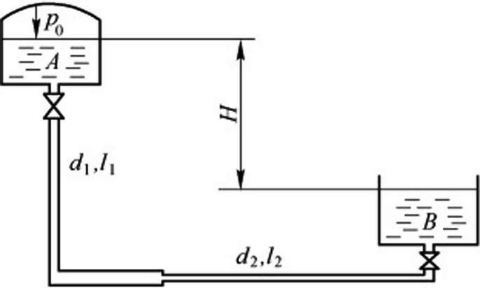
Problem 5.6
-
5.7
The pumping station utilizes a pipe with the diameter 60 cm to transport the water, and the friction loss is 27 m. To reduce the loss, another pipe with same length is connected in parallel with the first pipe, and correspondingly the total head loss decreases to 9.6 m. Assuming that both pipes have same friction factor and in either case, the total flow rate do not change. Find the diameter of second pipe.
-
5.8
As shown in Fig. 5.21, water flows from one reservoir to another. Assuming that \( H = 24\,\;{\text{m}} \), \( l_{1} = l_{2} = l_{3} = l_{4} = 100\,\;{\text{m}} \), \( d_{1} = d_{2} = d_{4} = 100\,\;{\text{mm}} \), \( d_{3} = 200\,\;{\text{mm}} \). The friction factor \( \lambda_{1} = \lambda_{2} = \lambda_{4} = 0.025 \), \( \lambda_{3} = 0.02 \). Except the minor head loss from valve, others can be neglected. Find: (1) the flow rate of the pipe when the minor loss coefficient of the valve is \( \zeta = 30 \). (2) the flow rate of the pipe when the valve is closed.
Fig. 5.21 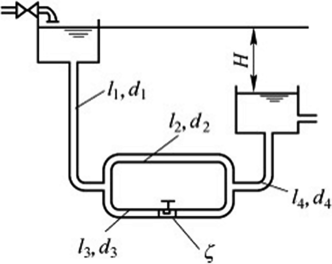
Problem 5.8
-
5.9
Assuming that there is steady discharge through a thin-plate orifice with the diameter \( d = 10\,\;{\text{mm}} \) in the tank. The flow rate is \( Q = 200\,\;{\text{cm}}^{ 3} / {\text{s}} \). Find the height H of the water in the tank.
-
5.10
As shown in Fig. 5.22, a reservoir is divided into two parts. Assuming that the diameter of small orifice is \( d = 200\,\;{\text{mm}} \), and \( v_{1} \approx v_{2} \approx 0 \). The water level difference from the upstream to the downstream is \( H = 2.5\,\;{\text{m}} \). Find the flow rate of the small orifice.
Fig. 5.22 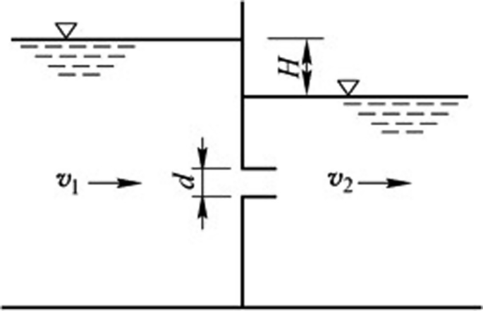
Problem 5.10
-
5.11
As shown in Fig. 5.23, there is a water tank with the height from the free surface to the bottom H, where the orifice on the side wall should be fixed in order to cover a maximum horizontal range for the jet. Find \( x_{\hbox{max} } \).
Fig. 5.23 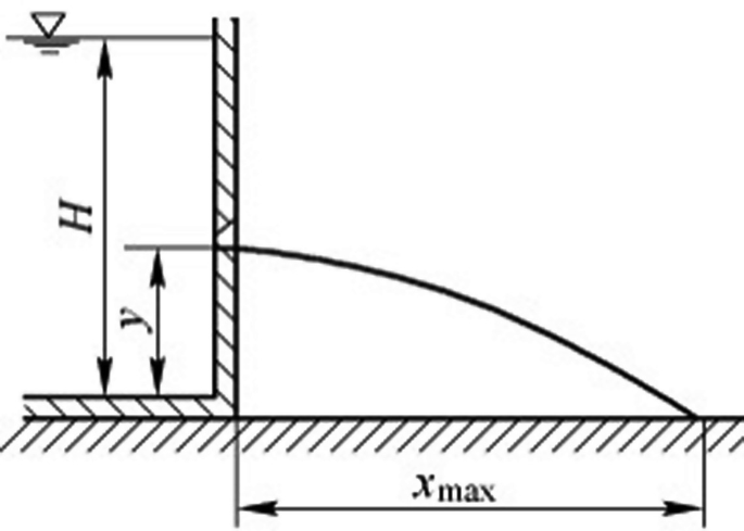
Problem 5.11
-
5.12
Assuming that the diameter of the orifice \( d = 100\,\;{\text{mm}} \), head \( H = 3\;{\text{m}} \). The velocity on vena contracta is \( v_{c} = 7\,\;{\text{m/s}} \), and the flow rate is \( Q = 36\,\;{\text{L/s}} \). Find: (1) the discharge coefficient for velocity \( \varphi \) and contraction coefficient \( \varepsilon \) of the orifice. (2) the flow rate if a cylindrical outer nozzle is connected to the orifice, and the discharge coefficient for flow rate is \( \mu = 0.82 \).
-
5.13
There is an enclosed container with liquid inside (the specific weight \( \gamma = 7850\,\;{\text{N/m}}^{ 3} \)). A cylindrical outer nozzle with the length \( l = 100\,\;{\text{mm}} \), the diameter \( d = 30\,\;{\text{mm}} \) is fixed on the section O–O, as shown in Fig. 5.24. The manometer is fixed 0.5 m higher than the section O–O with \( p_{M} = 4.9 \times 10^{4} \,\;{\text{Pa}} \). Find the velocity and the flow rate at starting time.
Fig. 5.24 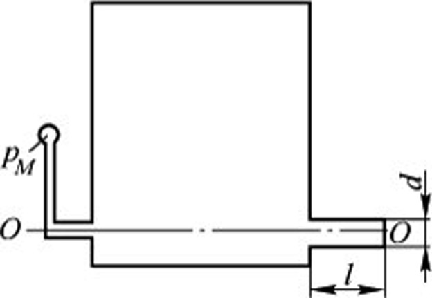
Problem 5.13
-
5.14
There is a rectangular tank with length \( l = 3\,\;{\text{m}} \), width \( B = 2\,{\text{m}} \), and depth of the water \( H = 1.5\,\;{\text{m}} \). Two orifices with the diameter \( d = 100\,\;{\text{mm}} \) are fixed at the bottom of the tank. Find the time when the free surface decreases 1 m.
-
5.15
As shown in Fig. 5.25, find the filling or emptying time of a chamber in ship lock. Assuming that the length and the width of the chamber are 68 m, 12 m respectively. The area of the upstream inlet orifice is 3.2 m2, and the height from the surface of the upstream to the centerline of the orifice is \( h = 4\,{\text{m}} \). The water level of the upstream and the downstream remain unchanged and their difference is \( H = 7.0\,\;{\text{m}} \).
Fig. 5.25 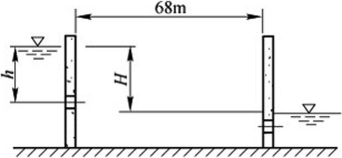
Problem 5.15


References
Song, H.: Engineering Fluid Mechanics and Environmental Application. Metallurgical Industry Press, Beijing (2016)
Xie, Z.: Engineering Fluid Mechanics, 4th edn. Metallurgical Industry Press, Beijing (2014)
White, F.M.: Fluid Mechanics, 7th edn. McGraw-Hill, New York (2011)
Fox, R.W., McDonald, A.T., Pritchard, P.J.: Introduction to Fluid Mechanics, vol. 5, 8th edn. Wiley, New York (2011)
Author information
Authors and Affiliations
Corresponding author
Rights and permissions
Copyright information
© 2018 Metallurgical Industry Press, Beijing and Springer Nature Singapore Pte Ltd.
About this chapter

Cite this chapter
Song, H. (2018). Pipe Network and Orifice, Nozzle Flow. In: Engineering Fluid Mechanics. Springer, Singapore. https://doi.org/10.1007/978-981-13-0173-5_5
Download citation
DOI: https://doi.org/10.1007/978-981-13-0173-5_5
Published:
Publisher Name: Springer, Singapore
Print ISBN: 978-981-13-0172-8
Online ISBN: 978-981-13-0173-5
eBook Packages: EngineeringEngineering (R0)