Step 5: Extracting Segments

Abstract

This chapter focuses on the task of grouping consumers and, in so doing, revealing naturally existing or creating artificial market segments. The chapter covers algorithms falling into three categories: distance-based methods, model-based methods, and algorithms integrating variable selection with the task of extracting market segments. In addition, data structure analysis is introduced. Data structure analysis provides insight into whether the resulting market segments are naturally occurring in the market; created but stable; or created and unstable across repeated calculations. A series of questions are included in a checklist to assist with the implementation of this step.

1 Grouping Consumers

Data-driven market segmentation analysis is exploratory by nature. Consumer data sets are typically not well structured. Consumers come in all shapes and forms; a two-dimensional plot of consumers’ product preferences typically does not contain clear groups of consumers. Rather, consumer preferences are spread across the entire plot. The combination of exploratory methods and unstructured consumer data means that results from any method used to extract market segments from such data will strongly depend on the assumptions made on the structure of the segments implied by the method. The result of a market segmentation analysis, therefore, is determined as much by the underlying data as it is by the extraction algorithm chosen. Segmentation methods shape the segmentation solution.

Many segmentation methods used to extract market segments are taken from the field of cluster analysis. In that case, market segments correspond to clusters. As pointed out by Hennig and Liao (2013), selecting a suitable clustering method requires matching the data analytic features of the resulting clustering with the context-dependent requirements that are desired by the researcher (p. 315). It is, therefore, important to explore market segmentation solutions derived from a range of different clustering methods. It is also important to understand how different algorithms impose structure on the extracted segments.

One of the most illustrative examples of how algorithms impose structure is shown in Fig. 7.1. In this figure, the same data set – containing two spiralling segments – is segmented using two different algorithms, and two different numbers of segments. The top row in Fig. 7.1 shows the market segments obtained when running k-means cluster analysis (for details see Sect. 7.2.3) with 2 (left) and 8 segments (right), respectively. As can be seen, k-means cluster analysis fails to identify the naturally existing spiral-shaped segments in the data. This is because k-means cluster analysis aims at finding compact clusters covering a similar range in all dimensions.

Fig. 7.1

k-means and single linkage hierarchical clustering of two spirals

The bottom row in Fig. 7.1 shows the market segments obtained from single linkage hierarchical clustering (for details see Sect. 7.2.2). This algorithm correctly identifies the existing two spiralling segments, even if the incorrect number of segments is specified up front. This is because the single linkage method constructs snake-shaped clusters. When asked to return too many (8) segments, outliers are defined as micro-segments, but the two main spirals are still correctly identified. k-means cluster analysis fails to identify the spirals because it is designed to construct round, equally sized clusters. As a consequence, the k-means algorithm ignores the spiral structure and, instead, places consumers in the same market segments if they are located close to one another (in Euclidean space), irrespective of the spiral they belong to.

This illustration gives the impression that single linkage clustering is much more powerful, and should be preferred over other approaches of extracting market segments from data. This is not the case. This particular data set was constructed specifically to play to the strengths of the single linkage algorithm allowing single linkage to identify the grouping corresponding to the spirals, and highlighting how critical the interaction between data and algorithm is. There is no single best algorithm for all data sets. If consumer data is well-structured, and well-separated, distinct market segments exist, tendencies of different algorithms matter less. If, however, data is not well-structured, the tendency of the algorithm influences the solution substantially. In such situations, the algorithm will impose a structure that suits the objective function of the algorithm.

The aim of this chapter is to provide an overview of the most popular extraction methods used in market segmentation, and point out their specific tendencies of imposing structure on the extracted segments. None of these methods outperform other methods in all situations. Rather, each method has advantages and disadvantages.

So-called distance-based methods are described first. Distance-based methods use a particular notion of similarity or distance between observations (consumers), and try to find groups of similar observations (market segments). So-called model-based methods are described second. These methods formulate a concise stochastic model for the market segments. In addition to those main two groups of extraction methods, a number of methods exist which try to achieve multiple aims in one step. For example, some methods perform variable selection during the extraction of market segments. A few such specialised algorithms are also discussed in this chapter.

Because no single best algorithm exists, investigating and comparing alternative segmentation solutions is critical to arriving at a good final solution. Data characteristics and expected or desired segment characteristics allow a pre-selection of suitable algorithms to be included in the comparison. Table 7.1 contains the information needed to guide algorithm selection.

Table 7.1 Data set and segment characteristics informing extraction algorithm selection

The size of the available data set indicates if the number of consumers is sufficient for the available number of segmentation variables, the expected number of segments, and the segment sizes. The minimum segment size required from a target segment has been defined as one of the knock-out criteria in Step 2. It informs the expectation about how many segments of which size will be extracted. If the target segment is expected to be a niche segment, larger sample sizes are required. Larger samples allow a more fine-grained extraction of segments. If the number of segmentation variables is large, but not all segmentation variables are expected to be key characteristics of segments, extraction algorithms which simultaneously select variables are helpful (see Sect. 7.4).

The scale level of the segmentation variables determines the most suitable variant of an extraction algorithms. For distance-based methods, the choice of the distance measure depends on the scale level of the data. The scale level also determines the set of suitable segment-specific models in the model-based approach. Other special structures of the data can restrict the set of suitable algorithms. If the data set contains repeated measurements of consumers over time, for example, an algorithm that takes this longitudinal nature of the data into account is needed. Such data generally requires a model-based approach.

We also need to specify the characteristics consumers should have in common to be placed in the same segment, and how they should differ from consumers in other segments. These features have, conceptually, been specified in Step 2, and need to be recalled here. The structure of segments extracted by the algorithm needs to align with these expected characteristics.

We distinguish directly observable characteristics from those that are only indirectly accessible. Benefits sought are an example of a directly observable characteristic. They are contained directly in the data, placing no restrictions on the segment extraction algorithm to be chosen. An example of an indirect characteristic is consumer price sensitivity. If the data contains purchase histories and price information, and market segments are based on similar price sensitivity levels, regression models are needed. This, in turn calls for the use of a model-based segment extraction algorithm.

In the case of binary segmentation variables, another aspect needs to be considered. We may want consumers in the same segments to have both the presence and absence of segmentation variables in common. In this case, we need to treat the binary segmentation variables symmetrically (with 0s and 1s treated equally). Alternatively, we may only care about segmentation variables consumers have in common. In this case, we treat them asymmetrically (with only common 1s being of interest). An example of where it makes sense to treat them asymmetrically is if we use vacation activities as the segmentation variables. It is very interesting if two tourists both engage in horse-riding during their vacation. It is not so interesting if two tourists do not engage in horse-riding. Biclustering (see Sect. 7.4.1) uses binary information asymmetrically. Distance-based methods can use distance measures that account for this asymmetry, and extract segments characterised by common 1s.

2 Distance-Based Methods

Consider the problem of finding groups of tourists with similar activity patterns when on vacation. A fictitious data set is shown in Table 7.2. It contains seven people indicating the percentage of time they spend enjoying beach, action, and culture when on vacation. Anna and Bill only want to relax on the beach, Frank likes beach and action, Julia and Maria like beach and culture, Michael wants action and a little bit of culture, and Tom does everything.

Table 7.2 Artificial data set on tourist activities: percentage of time spent on three activities

Market segmentation aims at grouping consumers into groups with similar needs or behaviour, in this example: groups of tourists with similar patterns of vacation activities. Anna and Bill have exactly the same profile, and should be in the same segment. Michael is the only one not interested in going to the beach, which differentiates him from the other tourists. In order to find groups of similar tourists one needs a notion of similarity or dissimilarity , mathematically speaking: a distance measure.

2.1 Distance Measures

Table 7.2 is a typical data matrix. Each row represents an observation (in this case a tourist), and every column represents a variable (in this case a vacation activity). Mathematically, this can be represented as an n × p matrix where n stands for the number of observations (rows) and p for the number of variables (columns):

$$\displaystyle \begin{aligned} \mathbf{X} = \left( \begin{array}{cccc} x_{11} & x_{12} & \cdots & x_{1p} \\ x_{21} & x_{22} & \cdots & x_{2p} \\ \vdots & \vdots & \ddots & \vdots \\ x_{n1} & x_{n2} & \cdots & x_{np} \end{array}\right)\end{aligned} $$

The vector corresponding to the i-th row of matrix X is denoted as x_i = (x_i1, x_i2, …, x_ip)′ in the following, such that $\mathcal {X} = \{{\mathbf {x}}_1, {\mathbf {x}}_2, \ldots {\mathbf {x}}_p\}$ is the set of all observations. In the example above, Anna’s vacation activity profile is vector x₁ = (100, 0, 0)′ and Tom’s vacation activity profile is vector x₇ = (50, 20, 30)′.

Numerous approaches to measuring the distance between two vectors exist; several are used routinely in cluster analysis and market segmentation. A distance is a function d(⋅, ⋅) with two arguments: the two vectors x and y between which the distance is being calculated. The result is the distance between them (a nonnegative value). A good way of thinking about distance is in the context of geography. If the distance between two cities is of interest, the location of the cities are the two vectors, and the length of the air route in kilometres is the distance. But even in the context of geographical distance, other measures of natural distance between two cities are equally valid, for example, the distance a car has to drive on roads to get from one city to the other.

A distance measure has to comply with a few criteria. One criterion is symmetry, that is:

$$\displaystyle \begin{aligned}d(\mathbf{x},\mathbf{y}) = d(\mathbf{y},\mathbf{x}).\end{aligned}$$

A second criterion is that the distance of a vector to itself and only to itself is 0:

$$\displaystyle \begin{aligned}d(\mathbf{x},\mathbf{y})=0\,\Leftrightarrow\,\mathbf{x}=\mathbf{y}.\end{aligned}$$

In addition, most distance measures fulfil the so-called triangle inequality:

$$\displaystyle \begin{aligned}d(\mathbf{x},\mathbf{z})\le d(\mathbf{x},\mathbf{y})+d(\mathbf{y},\mathbf{z}).\end{aligned}$$

The triangle inequality says that if one goes from x to z with an intermediate stop in y, the combined distance is at least as long as going from x to z directly.

Let x = (x₁, …, x_p)′ and y = (y₁, …, y_p)′ be two p-dimensional vectors. The most common distance measures used in market segmentation analysis are:

Euclidean distance: :

$$\displaystyle \begin{aligned} d(\mathbf{x}, \mathbf{y}) = \sqrt{\sum_{j=1}^p (x_j - y_j)^2} \end{aligned}$$

Manhattan or absolute distance: :

$$\displaystyle \begin{aligned} d(\mathbf{x}, \mathbf{y}) = \sum_{j=1}^p |x_j - y_j| \end{aligned}$$

Asymmetric binary distance: :

applies only to binary vectors, that is, all x_j and y_j are either 0 or 1.

$$\displaystyle \begin{aligned} d(\mathbf{x}, \mathbf{y}) = \left\{ \begin{array}{l} 0, \quad \mathbf{x} = \mathbf{y} = \mathbf{0} \\ (\#\{j| x_j=1 \mbox{ and } y_j=1\})/ (\#\{j| x_j=1 \mbox{ or } y_j=1\}) \end{array}\right. \end{aligned}$$

In words: the number of dimensions where both x and y are equal to 1 divided by the number of dimensions where at least one of them is 1.

Euclidean distance is the most common distance measure used in market segmentation analysis. Euclidean distance corresponds to the direct “straight-line” distance between two points in two-dimensional space, as shown in Fig. 7.2 on the left. Manhattan distance derives its name from the fact that it gives the distance between two points assuming that streets on a grid (like in Manhattan) need to be used to get from one point to another. Manhattan distance is illustrated in Fig. 7.2 on the right. Both Euclidean and Manhattan distance use all dimensions of the vectors x and y.

Fig. 7.2

A comparison of Euclidean and Manhattan distance

The asymmetric binary distance does not use all dimensions of the vectors. It only uses dimensions where at least one of the two vectors has a value of 1. It is asymmetric because it treats 0s and 1s differently. Similarity between two observations is only concluded if they share 1s, but not if they share 0s. The dissimilarity between two observations is increased if one has a 1 and the other not. This has implications for market segmentation analysis. Imagine, for example, that the tourist vacation activity profiles not only include common vacation activities, but also unusual activities, such as horseback riding and bungee jumping. The fact that two tourists have in common that they do not ride horses or that they do not bungee jump is not very helpful in terms of extracting market segments because the overall proportion of horse riders and bungee jumpers in the tourist population is low. If, however, two tourists do horse ride or bungee jump, this represents key information about similarities between them.

The asymmetric binary distance corresponds to the proportion of common 1s over all dimensions where at least one vector contains a 1. In the tourist example: the number of common vacation activities divided by the number of vacation activities at least one of the two tourists engages in. A symmetric binary distance measure (which treats 0s and 1s equally) emerges from using the Manhattan distance between the two vectors. The distance is then equal to the number of vacation activities where values are different.

The standard R function to calculate distances is called dist(). It takes as arguments a data matrix x and – optionally – the distance method. If no distance method is explicitly specified, Euclidean distance is the default. The R function returns all pairwise distances between the rows of x.

Using the vacation activity data in Table 7.2, we first need to load the data:

R> data("annabill", package = "MSA")

Then, we can calculate the Euclidean distance between all tourists with the following command:

R> D1 <- dist(annabill) R> round(D1, 2)

          Anna   Bill  Frank  Julia  Maria Michael Bill      0.00 Frank    56.57  56.57 Julia    42.43  42.43  50.99 Maria    28.28  28.28  48.99  14.14 Michael 134.91 134.91  78.74 115.76 120.83 Tom      61.64  61.64  37.42  28.28  37.42   88.32

The distance between Anna and Bill is zero because they have identical vacation activity profiles. The distance between Michael and all other people in the data set is substantial because Michael does not go to the beach where most other tourists spend a lot of time.

Manhattan distance – which is also referred to as absolute distance – is very similar to Euclidean distance for this data set:

R> D2 <- dist(annabill, method = "manhattan") R> D2

        Anna Bill Frank Julia Maria Michael Bill       0 Frank     80   80 Julia     60   60    80 Maria     40   40    80    20 Michael  200  200   120   180   180 Tom      100  100    60    40    60     140

No rounding is necessary because the Manhattan distance is automatically integer if all values in the data matrix are integer.

The printout contains only six rows and columns in both cases. To save computer memory, dist() does not return the full symmetric matrix of all pairwise distances. It only returns the lower triangle of the matrix. If the full matrix is required, it can be obtained by coercing the return object of dist() to the full 7 × 7 matrix:

R> as.matrix(D2)

        Anna Bill Frank Julia Maria Michael Tom Anna       0    0    80    60    40     200 100 Bill       0    0    80    60    40     200 100 Frank     80   80     0    80    80     120  60 Julia     60   60    80     0    20     180  40 Maria     40   40    80    20     0     180  60 Michael  200  200   120   180   180       0 140 Tom      100  100    60    40    60     140   0

Both Euclidean and Manhattan distance treat all dimensions of the data equally; they take a sum over all dimensions of squared or absolute differences. If the different dimensions of the data are not on the same scale (for example, dimension 1 indicates whether or not a tourist plays golf, and dimension 2 indicates how many dollars the tourist spends per day on dining out on average), the dimension with the larger numbers will dominate the distance calculation between two observations. In such situations data needs to be standardised before calculating distances (see Sect. 6.4.2).

Function dist can only be used if the segmentation variables are either all metric or all binary. In R package cluster (Maechler et al. 2017), function daisy calculates the dissimilarity matrix between observations contained in a data frame. In this data frame the variables can be numeric, ordinal, nominal and binary. Following Gower (1971), all variables are rescaled to a range of [0, 1] which allows for a suitable weighting between variables. If variables are metric, the results are the same as for dist:

R> library("cluster") R> round(daisy(annabill), digits = 2)

Dissimilarities :           Anna   Bill  Frank  Julia  Maria Michael Bill      0.00 Frank    56.57  56.57 Julia    42.43  42.43  50.99 Maria    28.28  28.28  48.99  14.14 Michael 134.91 134.91  78.74 115.76 120.83 Tom      61.64  61.64  37.42  28.28  37.42   88.32 Metric :  euclidean Number of objects : 7

2.2 Hierarchical Methods

Hierarchical clustering methods are the most intuitive way of grouping data because they mimic how a human would approach the task of dividing a set of n observations (consumers) into k groups (segments). If the aim is to have one large market segment (k = 1), the only possible solution is one big market segment containing all consumers in data $\mathcal {X}$. At the other extreme, if the aim is to have as many market segments as there are consumers in the data set (k = n), the number of market segments has to be n, with each segment containing exactly one consumer. Each consumer represents their own cluster. Market segmentation analysis occurs between those two extremes.

Divisive hierarchical clustering methods start with the complete data set $\mathcal {X}$ and splits it into two market segments in a first step. Then, each of the segments is again split into two segments. This process continues until each consumer has their own market segment.

Agglomerative hierarchical clustering approaches the task from the other end. The starting point is each consumer representing their own market segment (n singleton clusters). Step-by-step, the two market segments closest to one another are merged until the complete data set forms one large market segment.

Both approaches result in a sequence of nested partitions. A partition is a grouping of observations such that each observation is exactly contained in one group. The sequence of partitions ranges from partitions containing only one group (segment) to n groups (segments). They are nested because the partition with k + 1 groups (segments) is obtained from the partition with k groups by splitting one of the groups.

Numerous algorithms have been proposed for both strategies. The unifying framework for agglomerative clustering – which was developed in the seminal paper by Lance and Williams (1967) – contains most methods still in use today. In each step, standard implementations of hierarchical clustering perform the optimal step. This leads to a deterministic algorithm. This means that every time the hierarchical clustering algorithm is applied to the same data set, the exactly same sequence of nested partitions is obtained. There is no random component.

Underlying both divisive and agglomerative clustering is a measure of distance between groups of observations (segments). This measure is determined by specifying (1) a distance measure d(x, y) between observations (consumers) x and y, and (2) a linkage method . The linkage method generalises how, given a distance between pairs of observations, distances between groups of observations are obtained. Assuming two sets $\mathcal {X}$ and $\mathcal {Y}$ of observations (consumers), the following linkage methods are available in the standard R function hclust() for measuring the distance $l(\mathcal {X},\mathcal {Y})$ between these two sets of observations:

Single linkage: :

distance between the two closest observations of the two sets.

$$\displaystyle \begin{aligned} l(\mathcal{X},\mathcal{Y}) = \min_{\mathbf{x}\in \mathcal{X}, \mathbf{y}\in \mathcal{Y}} d(\mathbf{x},\mathbf{y}) \end{aligned}$$

Complete linkage: :

distance between the two observations of the two sets that are farthest away from each other.

$$\displaystyle \begin{aligned} l(\mathcal{X},\mathcal{Y}) = \max_{\mathbf{x}\in \mathcal{X}, \mathbf{y}\in \mathcal{Y}} d(\mathbf{x},\mathbf{y}) \end{aligned}$$

Average linkage: :

mean distance between observations of the two sets.

$$\displaystyle \begin{aligned} l(\mathcal{X},\mathcal{Y}) = \frac 1{|\mathcal{X}||\mathcal{Y}|}\sum_{\mathbf{x}\in \mathcal{X}} \sum_{\mathbf{y}\in \mathcal{Y}} d(\mathbf{ x},\mathbf {y}), \end{aligned}$$

where $|\mathcal {X}|$ denotes the number of elements in $\mathcal {X}$.

These linkage methods are illustrated in Fig. 7.3, and all of them can be combined with any distance measure. There is no correct combination of distance and linkage method. Clustering in general, and hierarchical clustering in specific, are exploratory techniques. Different combinations can reveal different features of the data.

Fig. 7.3

A comparison of different linkage methods between two sets of points

Single linkage uses a “next neighbour” approach to join sets, meaning that the two closest consumers are united. As a consequence, single linkage hierarchical clustering is capable of revealing non-convex, non-linear structures like the spirals in Fig. 7.1. In situations where clusters are not well-separated – and this means in most consumer data situations – the next neighbour approach can lead to undesirable chain effects where two groups of consumers form a segment only because two consumers belonging to each of those segments are close to one another. Average and complete linkage extract more compact clusters.

A very popular alternative hierarchical clustering method is named after Ward (1963), and based on squared Euclidean distances. Ward clustering joins the two sets of observations (consumers) with the minimal weighted squared Euclidean distance between cluster centers. Cluster centers are the midpoints of each cluster. They result from taking the average over the observations in the cluster. We can intepret them as segment representatives.

When using Ward clustering we need to check that the correct distance is used as input (Murtagh and Legendre 2014). The two options are Euclidean distance or squared Euclidean distance. Function hclust() in R can deal with both kinds of input. The input, along with the suitable linkage method, needs to be specified in the R command as either Euclidean distance with method = "ward.D2", or as squared Euclidean distance with method = "ward.D" The result of hierarchical clustering is typically presented as a dendrogram . A dendrogram is a tree diagram. The root of the tree represents the one-cluster solution where one market segment contains all consumers. The leaves of the tree are the single observations (consumers), and branches in-between correspond to the hierarchy of market segments formed at each step of the procedure. The height of the branches corresponds to the distance between the clusters. Higher branches point to more distinct market segments. Dendrograms are often recommended as a guide to select the number of market segments. Based on the authors’ experience with market segmentation analysis using consumer data, however, dendrograms rarely provide guidance of this nature because the data sets underlying the analysis are not well structured enough.

As an illustration of the dendrogram, consider the seven tourists in Table 7.2 and the Manhattan distances between them. Agglomerative hierarchical clustering with single linkage will first identify the two people with the smallest distance (Anna and Bill with a distance of 0). Next, Julia and Maria are joined into a market segment because they have the second smallest distance between them (20). The single linkage distance between these two groups is 40, because that is the distance from Maria to Anna and Bill. Tom has a distance of 40 to Julia, hence Anna, Bill, Julia, Maria and Tom are joined to a group of five in the third step. This process continues until all tourists are united in one big group. The resulting dendrogram is shown in Fig. 7.4 on the left.

Fig. 7.4

Single and complete linkage clustering of the tourist data shown in Table 7.2

The result of complete linkage clustering is provided in the right dendrogram in Fig. 7.4. For this small data set, the result is very similar. The only major difference is that Frank and Tom are first grouped together in a segment of two, before they are merged into a segment with all other tourists (except for Michael) in the data set. In both cases, Michael is merged last because his activity profile is very different. The result from average linkage clustering is not shown because the corresponding dendrogram is almost identical to that of complete linkage clustering.

The order of the leaves of the tree (the observations or consumers) is not unique. At every split into two branches, the left and right branch could be exchanged, resulting in 2ⁿ possible dendrograms for exactly the same clustering where n is the number of consumers in the data set. As a consequence, dendrograms resulting from different software packages may look different although they represent exactly the same market segmentation solution. Another possible source of variation between software packages is how ties are broken, meaning, which two groups are joined first when several have exactly the same distance .

Example: Tourist Risk Taking

A data set on “tourist disasters” contains survey data collected by an online research panel company in October 2015 commissioned by UQ Business School (Hajibaba et al. 2017). The target population were adult Australian residents who had undertaken at least one personal holiday in the past 12 months. The following commands load the data matrix:

R> library("MSA") R> data("risk", package = "MSA") R> dim(risk)

[1] 563   6

This data set contains 563 respondents who state how often they take risks from the following six categories:

• 1. recreational risks: e.g., rock-climbing, scuba diving

• 2. health risks: e.g., smoking, poor diet, high alcohol consumption

• 3. career risks: e.g., quitting a job without another to go to

• 4. financial risks: e.g., gambling, risky investments

• 5. safety risks: e.g., speeding

• 6. social risks: e.g., standing for election, publicly challenging a rule or decision

Respondents are presented with an ordinal scale consisting of five answer options (1=never, 5=very often). In the subsequent analysis, we assume equidistance between categories. Respondents, on average, display risk aversion with mean values for all columns close to 2 (=rarely):

R> colMeans(risk)

Recreational       Health       Career    Financial     2.190053     2.396092     2.007105     2.026643       Safety       Social     2.266430     2.017762

The following command extracts market segments from this data set using Manhattan distance and complete linkage :

R> risk.dist <- dist(risk, method = "manhattan") R> risk.hcl <- hclust(risk.dist, method = "complete") R> risk.hcl

Call: hclust(d = risk.dist, method = "complete") Cluster method   : complete Distance         : manhattan Number of objects: 563

plot(risk.hcl) generates the dendrogram shown in Fig. 7.5. The dendrogram visualises the sequence of nested partitions by indicating each merger or split. The straight line at the top of the dendrogram indicates the merger of the last two groups into a single group. The y-axis indicates the distance between these two groups. At the bottom each single observation is one line.

Fig. 7.5

Complete linkage hierarchical cluster analysis of the tourist risk taking data set

The dendrogram in Fig. 7.5 indicates that the largest additional distance between two clusters merged occurred when the last two clusters were combined to the single cluster containing all observations. Cutting the dendrogram at a specific height selects a specific partition. The boxes numbered 1–6 in Fig. 7.5 illustrate how this dendrogram or tree can be cut into six market segments. The reason that the boxes are not numbered from left to right is that the market segment labelled number 1 contains the first observation (the first consumer) in the data set. Which consumers have been assigned to which market segment can be computed using function cutree(), which takes an object as returned by hclust and either the height h at which to cut or the number k of segments to cut the tree into.

R> c2 <- cutree(risk.hcl, h = 20) R> table(c2)

c2   1   2 511  52

R> c6 <- cutree(risk.hcl, k = 6) R> table(c6)

c6   1   2   3   4   5   6  90 275  27  25  74  72

A simple way to assess the characteristics of the clusters is to look at the column-wise means by cluster.

R> c6.means <- aggregate(risk, list(Cluster = c6), mean) R> round(c6.means, 1)

  Recreational Health Career Financial Safety Social 1          2.0    2.2    1.9       2.0    2.2    2.8 2          1.9    1.8    1.5       1.6    2.0    1.4 3          3.9    4.4    2.9       3.2    3.3    4.1 4          4.1    3.3    4.1       2.8    3.4    3.2 5          2.3    2.6    3.2       2.6    2.6    2.2 6          2.0    3.8    1.8       2.4    2.3    2.0

But it is much easier to understand the cluster characteristics by visualising the column-wise means by clusters using a barchart (Fig. 7.6). barchart(risk. hcl, risk, k=6) from R package flexclust results in such a barchart. (A refined version of this plot – referred to as the segment profile plot – is described in detail in Sect. 8.3). The dark red dots correspond to the total mean values across all respondents; the bars indicate the mean values within each one of the segments. Segments are interpreted by inspecting the difference between the total population (red dots) and the segments (bars). For the tourist risk taking data set, the largest segment is cluster 2. People assigned to this segment avoid all types of risks as indicated by all bars being lower than all the red dots. Segments 3 and 4 display above average risk taking in all areas, while segments 1, 5 and 6 have average risk taking values for 5 of the 6 categories, but are characterised by their willingness to take above average risk in one category. Members of segment 1 are more willing to accept social risks than the overall population, members of segment 5 are more willing to accept career risks, and members of segment 6 are more willing to accept health risks.

Fig. 7.6

Bar chart of cluster means from hierarchical clustering for the tourist risk taking data set

2.3 Partitioning Methods

Hierarchical clustering methods are particularly well suited for the analysis of small data sets with up to a few hundred observations. For larger data sets, dendrograms are hard to read, and the matrix of pairwise distances usually does not fit into computer memory. For data sets containing more than 1000 observations (consumers), clustering methods creating a single partition are more suitable than a nested sequence of partitions. This means that – instead of computing all distances between all pairs of observations in the data set at the beginning of a hierarchical partitioning cluster analysis using a standard implementation – only distances between each consumer in the data set and the centre of the segments are computed. For a data set including information about 1000 consumers, for example, the agglomerative hierarchical clustering algorithm would have to calculate (1000 × 999)∕2 = 499, 500 distances for the pairwise distance matrix between all consumers in the data set.

A partitioning clustering algorithm aiming to extract five market segments, in contrast, would only have to calculate between 5 and 5000 distances at each step of the iterative or stepwise process (the exact number depends on the algorithm used). In addition, if only a few segments are extracted, it is better to optimise specifically for that goal, rather than building the complete dendrogram and then heuristically cutting it into segments.

2.3.1 k-Means and k-Centroid Clustering

The most popular partitioning method is k-means clustering. Within this method, a number of algorithms are available. R function kmeans() implements the algorithms by Forgy (1965), Hartigan and Wong (1979), Lloyd (1982) and MacQueen (1967). These algorithms use the squared Euclidean distance . A generalisation to other distance measures, also referred to as k-centroid clustering, is provided in R package flexclust.

Let $\mathcal {X} = \{{\mathbf {x}}_1,\ldots ,{\mathbf {x}}_n\}$ be a set of observations (consumers) in a data set. Partitioning clustering methods divide these consumers into subsets (market segments) such that consumers assigned to the same market segment are as similar to one another as possible, while consumers belonging to different market segments are as dissimilar as possible. The representative of a market segment is referred to in many partitioning clustering algorithms as the centroid . For the k-means algorithm based on the squared Euclidean distance , the centroid consists of the column-wise mean values across all members of the market segment. The data set contains observations (consumers) in rows, and variables (behavioural information or answers to survey questions) in columns. The column-wise mean, therefore, is the average response pattern across all segmentation variables for all members of the segment (Fig. 7.6).

The following generic algorithm represents a heuristic for solving the optimisation problem of dividing consumers into a given number of segments such that consumers are similar to their fellow segment members, but dissimilar to members of other segments. This algorithm is iterative; it improves the partition in each step, and is bound to converge, but not necessarily to the global optimum .

It involves five steps with the first four steps visualised in a simplified way in Fig. 7.7:

• 1. Specify the desired number of segments k.

  Fig. 7.7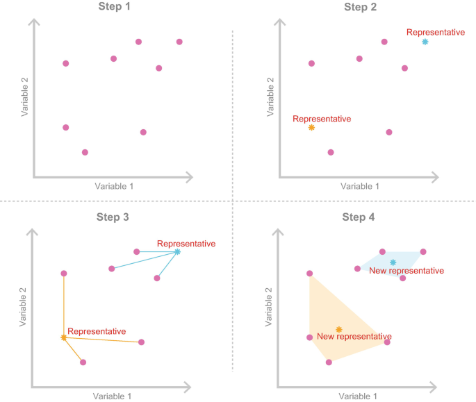

  

  Simplified visualisation of the k-means clustering algorithm

• 2. Randomly select k observations (consumers) from data set $\mathcal {X}$ (see Step 2 in Fig. 7.7) and use them as initial set of cluster centroids $\mathcal {C}=\{{\mathbf {c}}_1,\ldots ,{\mathbf {c}}_k\}$. If five market segments are being extracted, then five consumers are randomly drawn from the data set, and declared the representatives of the five market segments. Of course, these randomly chosen consumers will – at this early stage of the process – not be representing the optimal segmentation solution. They are needed to get the step wise (iterative) partitioning algorithm started.

• 3. Assign each observation x_i to the closest cluster centroid (segment representative, see Step 3 in Fig. 7.7) to form a partition of the data, that is, k market segments $\mathcal {S}_1,\ldots ,\mathcal {S}_k$ where

  $$\displaystyle \begin{aligned}\mathcal{S}_j = \{\mathbf{x}\in\mathcal{X}|d(\mathbf{x},{\mathbf{c}}_j)\le d(\mathbf{x},{\mathbf{c}}_h),\;1\le h\le k\}.\end{aligned} $$

  This means that each consumer in the data set is assigned to one of the initial segment representatives. This is achieved by calculating the distance between each consumer and each segment representative, and then assigning the consumer to the market segment with the most similar representative. If two segment representatives are equally close, one needs to be randomly selected. The result of this step is an initial – suboptimal – segmentation solution. All consumers in the data set are assigned to a segment. But the segments do not yet comply with the criterion that members of the same segment are as similar as possible, and members of different segments are as dissimilar as possible.

• 4. Recompute the cluster centroids (segment representatives) by holding cluster membership fixed, and minimising the distance from each consumer to the corresponding cluster centroid (representative see Step 4 in Fig. 7.7):

  $$\displaystyle \begin{aligned}{\mathbf{c}}_j = \arg\min_{\mathbf{c}} \sum_{\mathbf{x}\in\mathcal{S}_j} d(\mathbf{x},\mathbf{ c}).\end{aligned}$$

  For squared Euclidean distance , the optimal centroids are the cluster-wise means, for Manhattan distance cluster-wise medians, resulting in the so-called k-means and k-medians procedures, respectively. In less mathematical terms: what happens here is that – acknowledging that the initial segmentation solution is not optimal – better segment representatives need to be identified. This is exactly what is achieved in this step: using the initial segmentation solution, one new representative is “elected” for each of the market segments. When squared Euclidean distance is used, this is done by calculating the average across all segment members, effectively finding the most typical, hypothetical segment members and declaring them to be the new representatives.

• 5. Repeat from step 3 until convergence or a pre-specified maximum number of iterations is reached. This means that the steps of assigning consumers to their closest representative, and electing new representatives is repeated until the point is reached where the segment representatives stay the same. This is when the stepwise process of the partitioning algorithm stops and the segmentation solution is declared to be the final one.

The algorithm will always converge: the stepwise process used in a partitioning clustering algorithm will always lead to a solution. Reaching the solution may take longer for large data sets, and large numbers of market segments, however. The starting point of the process is random. Random initial segment representatives are chosen at the beginning of the process. Different random initial representatives (centroids) will inevitably lead to different market segmentation solutions. Keeping this in mind is critical to conducting high quality market segmentation analysis because it serves as a reminder that running one single calculation with one single algorithm leads to nothing more than one out of many possible segmentation solutions. The key to a high quality segmentation analysis is systematic repetition, enabling the data analyst to weed out less useful solutions, and present to the users of the segmentation solution – managers of the organisation wanting to adopt target marketing – the best available market segment or set of market segments.

In addition, the algorithm requires the specification of the number of segments. This sounds much easier than it is. The challenge of determining the optimal number of market segments is as old as the endeavour of grouping people into segments itself (Thorndike 1953). A number of indices have been proposed to assist the data analyst (these are discussed in detail in Sect. 7.5.1). We prefer to assess the stability of different segmentation solutions before extracting market segments. The key idea is to systematically repeat the extraction process for different numbers of clusters (or market segments), and then select the number of segments that leads to either the most stable overall segmentation solution, or to the most stable individual segment. Stability analysis is discussed in detail in Sects. 7.5.3 and 7.5.4. In any case, partitioning clustering does require the data analyst to specify the number of market segments to be extracted in advance.

What is described above is a generic version of a partitioning clustering algorithm. Many variations of this generic algorithm are available; some are discussed in the subsequent subsections. The machine learning community has also proposed a number of clustering algorithms. Within this community, the term unsupervised learning is used to refer to clustering because groups of consumers are created without using an external (or dependent) variable. In contrast, supervised learning methods use a dependent variable. The equivalent statistical methods are regression (when the dependent variable is metric), and classification (when the dependent variable is nominal). Hastie et al. (2009) discuss the relationships between statistics and machine learning in detail. Machine learning algorithms essentially achieve the same thing as their statistical counterparts. The main difference is in the vocabulary used to describe the algorithms.

Irrespective of whether traditional statistical partitioning methods such as k-means are used, or whether any of the algorithms proposed by the machine learning community is applied, distance measures are the basic underlying calculation. Not surprisingly, therefore, the choice of the distance measure has a significant impact on the final segmentation solution. In fact, the choice of the distance measure typically has a bigger impact on the nature of the resulting market segmentation solution than the choice of algorithm (Leisch 2006). To illustrate this, artificial data from a bivariate normal distribution are clustered three times using a generalised version of the k-means algorithm. A different distance measure is used for each calculation: squared Euclidean distance, Manhattan distance, and the difference between angles when connecting observations to the origin.

Figure 7.8 shows the resulting three partitions. As can be seen, squared Euclidean and Manhattan distance result in similarly shaped clusters in the interior of the data. The direction of cluster borders in the outer region of the data set, however, are quite different. Squared Euclidean distance results in diagonal borders, while the borders for Manhattan distance are parallel to the axes. Angle distance slices the data set into cake piece shaped segments. Figure 7.8 shows clearly the effect of the chosen distance measure on the segmentation solution. Note, however, that – while the three resulting segmentation solutions are different – neither of them is superior or inferior, especially given that no natural clusters are present in this data set.

Fig. 7.8

Artificial Gaussian data clustered using squared Euclidean distance (left), Manhattan distance (middle) and angle distance (right)

2.3.1.1 Example: Artificial Mobile Phone Data

Consider a simple artificial data set for a hypothetical mobile phone market. It contains two pieces of information about mobile phone users: the number of features they want in a mobile phone, and the price they are willing to pay for it. We can artificially generate a random sample for such a scenario in R. To do this, we first load package flexclust which also contains a wide variety of partitioning clustering algorithms for many different distance measures:

R> library("flexclust") R> set.seed(1234) R> PF3 <- priceFeature(500, which = "3clust")

Next, we set the seed of the random number generator to 1234. We use seed 1234 throughout the book whenever randomness is involved to make all results reproducible. After setting the seed of the random number generator, it always produces exactly the same sequence of numbers. In the example above, function priceFeature() draws a random sample with uniform distribution on three circles. Data sets drawn with different seeds will all look very similar, but the exact location of points is different.

Figure 7.9 shows the data. The x-axis plots mobile phone features. The y-axis plots the price mobile phone users are willing to pay. The data contains three very distinct and well-separated market segments. Members of the bottom left market segment want a cheap mobile phone with a limited set of features. Members of the middle segment are willing to pay a little bit more, and expect a few additional features. Members of the small market segment located in the top right corner of Fig. 7.9 are willing to pay a lot of money for their mobile phone, but have very high expectations in terms of features.

Fig. 7.9

Artificial mobile phone data set

Next, we extract market segments from this data. Figure 7.9 shows clearly that three market segments exist (when working with empirical data it is not known how many, if any, natural segments are contained in the data). To obtain a solution containing three market segments for the artificially generated mobile phone data set using k-means , we use function cclust() from package flexclust. Compared to the standard R function kmeans(), function cclust() returns richer objects, which are useful for the subsequent visualisation of results using tools from package flexclust. Function cclust() implements the k-means algorithm by determining the centroids using the average values across segment members, and by assigning each observation to the closest centroid using Euclidean distance.

R> PF3.km3 <- cclust(PF3, k = 3) R> PF3.km3

kcca object of family ’kmeans’ call: cclust(x = PF3, k = 3) cluster sizes:   1   2   3 100 200 200

The cluster centres (centroids, representatives of each market segment), and the vector of cluster memberships (the assignment of each consumer to a specific market segment) can be extracted using

R> parameters(PF3.km3)

     features / performance / quality    price [1,]                         7.976827 8.027105 [2,]                         5.021999 4.881439 [3,]                         1.990105 2.062453

R> clusters(PF3.km3)[1:20]

 [1] 1 2 3 3 2 3 2 3 1 1 3 1 3 2 2 3 2 1 2 1

The term [1:20] in the above R command asks for the segment memberships of only the first 20 consumers in the data set to be displayed (to save space). The numbering of the segments (clusters) is random; it depends on which consumers from the data set have been randomly chosen to be the initial segment representatives. Exactly the same solution could be obtained with a different numbering of segments; the market segment labelled cluster 1 in one calculation could be labelled cluster 3 in the next calculation, although the grouping of consumers is the same.

The information about segment membership can be used to plot market segments in colour, and to draw circles around them. These circles are referred to as convex hulls. In two-dimensional space, the convex hull of a set of observations is a closed polygon connecting the outer points in a way that ensures that all points of the set are located within the polygon. An additional requirement is that the polygon has no “inward dents”. This means that any line connecting two data points of the set must not lie outside the convex hull. To generate a coloured scatter plot of the data with convex hulls for the segments – such as the one depicted in Fig. 7.10 – we can use function clusterhull() from package MSA:

Fig. 7.10

Three-segment k-means partition for the artificial mobile phone data set

R> clusterhulls(PF3, clusters(PF3.km3))

Figure 7.10 visualises the segmentation solution resulting from a single run of the k-means algorithm with one specific set of initial segment representatives. The final segmentation solution returned by the k-means algorithm differs for different initial values. Because each calculation starts with randomly selected consumers serving as initial segment representatives, it is helpful to rerun the process of selecting random segment representatives a few times to eliminate a particularly bad initial set of segment representatives. The process of selecting random segment representatives is called random initialisation .

Specifying the number of clusters (number of segments ) is difficult because, typically, consumer data does not contain distinct, well-separated naturally existing market segments. A popular approach is to repeat the clustering procedure for different numbers of market segments (for example: everything from two to eight market segments), and then compare – across those solutions – the sum of distances of all observations to their representative. The lower the distance, the better the segmentation solution because members of market segments are very similar to one another.

We now calculate 10 runs of the k-means algorithm for each number of segments using different random initial representatives (nrep = 10), and retain the best solution for each number of segments. The number of segments varies from 2 to 8 (k = 2:8):

R> PF3.km28 <- stepcclust(PF3, k = 2:8, nrep = 10)

2 : ∗ ∗ ∗ ∗ ∗ ∗ ∗ ∗ ∗ ∗ 3 : ∗ ∗ ∗ ∗ ∗ ∗ ∗ ∗ ∗ ∗ 4 : ∗ ∗ ∗ ∗ ∗ ∗ ∗ ∗ ∗ ∗ 5 : ∗ ∗ ∗ ∗ ∗ ∗ ∗ ∗ ∗ ∗ 6 : ∗ ∗ ∗ ∗ ∗ ∗ ∗ ∗ ∗ ∗ 7 : ∗ ∗ ∗ ∗ ∗ ∗ ∗ ∗ ∗ ∗ 8 : ∗ ∗ ∗ ∗ ∗ ∗ ∗ ∗ ∗ ∗

R> PF3.km28

stepFlexclust object of family ’kmeans’ call: stepcclust(PF3, k = 2:8, nrep = 10)   iter converged   distsum 1   NA        NA 1434.6462 2    5      TRUE  827.6455 3    3      TRUE  464.7213 4    4      TRUE  416.6217 5   11      TRUE  374.4978 6   11      TRUE  339.6770 7   12      TRUE  313.8717 8   15      TRUE  284.9730

In this case, we extract market segmentation solutions containing between 2 and 8 segments (argument k = 2:8). For each one of those solutions, we retain the best out of ten random initialisations (nrep = 10), using the sum of Euclidean distances between the segment members and their segment representatives as criterion.

Function stepcclust() enables automated parallel processing on multiple cores of a computer (see help("stepcclust") for details). This is useful because the repeated calculations for different numbers of segments and different random initialisations are independent. In the example above 7 × 10 = 70 segment extractions are required. Without parallel computing, these 70 segment extractions run sequentially one after the other. Parallel computing means that a number of calculations can run simultaneously. Parallel computing is possible on most modern standard laptops, which can typically run at least four R processes in parallel, reducing the required runtime of the command by a factor of four (e.g., 15 s instead of 60 s). More powerful desktop machines or compute servers allow many more parallel R processes. For single runs of stepcclust() this makes little difference, but as soon as advanced bootstrapping procedures are used, the difference in runtime can be substantial. Calculations which would run for an hour, are processed in 15 min on a laptop, and in 1.5 min on a computer server running 40 parallel processes. The R commands used are exactly the same, but parallel processing needs to be enabled before using them. The help page for function stepcclust() offers examples on how to do that.

The sums of within-cluster distances for different numbers of clusters (number of market segments ) are visualised using plot(PF3.km28). Figure 7.11 shows the resulting scree plot. The scree plot displays – for each number of segments – the sum of within-cluster distances. For clustering results obtained using stepcclust, this is the sum of the Euclidean distances between each segment member and the representative of the segment. The smaller this number, the more homogeneous the segments; members assigned to the same market segment are similar to one another. Optimally, the scree plot shows distinct drops in the sum of within-cluster distances for the first numbers of segments, followed only by small decreases afterwards. The number of segments where the last distinct drop occurs is the optimal number of segments. After this point, homogeneous segments are split up artificially, resulting in no major decreases in the sum of within-cluster distances.

Fig. 7.11

Scree plot for k-means partitions with k = 1, …, 8 segments for the artificial mobile phone data set

The point of the scree plot indicating the best number of segments is where an elbow occurs. The elbow is illustrated in Fig. 7.12. Figure 7.12 contains the scree plot as well as an illustration of the elbow. The elbow is visualised by the two intersecting lines with different slopes. The point where the two lines intersect indicates the optimal number of segments. In the example shown in Fig. 7.12, large distance drops are visible when the number of segments increases from one to two segments, and then again from two to three segments. A further increase in segments leads to small reductions in distance.

Fig. 7.12

Scree plot for k-means partitions with k = 1, …, 8 segments for the artificial mobile phone data set including a visualisation of the elbow consisting of two intersecting lines with different slopes

For this simple artificial data set – constructed to contain three distinct and exceptionally well-separated market segments – the scree plot in Fig. 7.11 correctly points to three market segments being a good choice. The scree plot only provides guidance if market segments are well-separated. If they are not, stability analysis – discussed in detail in Sects. 7.5.3 and 7.5.4 – can inform the number of segments decision.

2.3.1.2 Example: Tourist Risk Taking

To illustrate the difference between an artificially created data set (containing three textbook market segments), and a data set containing real consumer data, we use the tourist risk taking data set. We generate solutions for between 2 and 8 segments (k = 2, …, 8 clusters) using the following command:

R> set.seed(1234) R> risk.km28 <- stepcclust(risk, k = 2:8, nrep = 10)

We use the default seed of 1234 for the random number generator, and initialise each k-means run with a different set of k random representatives. To make it possible for readers to get exactly the same results as shown in this book, the seed is actively set. Figure 7.13 contains the corresponding sum of distances . As can be seen immediately, the drops in distances are much less distinct for this consumer data set than they were for the artificial mobile phone data set. No obvious number of segments recommendation emerges from this plot. But if this plot were the only available decision tool, the two-segment solution would be chosen. We obtain the corresponding bar chart using

Fig. 7.13

Scree plot for k-means partitions with k = 1, …, 8 segments for the tourist risk taking data set

R> barchart(risk.km28[["2"]])

(Figure not shown). The solution containing two market segments splits the data into risk-averse people and risk-takers, reflecting the two main branches of the dendrogram in Fig. 7.5.

Figure 7.14 show the six-segment solution. It is similar to the partition resulting from the hierarchical clustering procedure, but not exactly the same. The six-segment solution resulting from the partitioning algorithm contains two segments of low risk takers (segments 1 and 4), two segments of high risk takers (segments 2 and 5), and two distinctly profiled segments, one of which contains people taking recreational and social risks (segment 3), and another one containing health risk takers (segment 6). Both partitions obtained using either hierarchical or partitioning clustering methods are reasonable from a statistical point of view. Which partition is more suitable to underpin the market segmentation strategy of an organisation needs to be evaluated jointly by the data analyst and the user of the segmentation solution using the tools and methods presented in Sect. 7.5 and in Steps 6, 7 and 8.

Fig. 7.14

Bar chart of cluster means from k-means clustering for the tourist risk taking data set

2.3.2 “Improved” k-Means

Many attempts have been made to refine and improve the k-means clustering algorithm. The simplest improvement is to initialise k-means using “smart” starting values, rather than randomly drawing k consumers from the data set and using them as starting points. Using randomly drawn consumers is suboptimal because it may result in some of those randomly drawn consumers being located very close to one another, and thus not being representative of the data space. Using starting points that are not representative of the data space increases the likelihood of the k-means algorithm getting stuck in what is referred to as a local optimum. A local optimum is a good solution, but not the best possible solution. One way of avoiding the problem of the algorithm getting stuck in a local optimum is to initialise it using starting points evenly spread across the entire data space. Such starting points better represent the entire data set.

Steinley and Brusco (2007) compare 12 different strategies proposed to initialise the k-means algorithm. Based on an extensive simulation study using artificial data sets of known structure, Steinley and Brusco conclude that the best approach is to randomly draw many starting points, and select the best set. The best starting points are those that best represent the data. Good representatives are close to their segment members; the total distance of all segment members to their representatives is small (as illustrated on the left side of Fig. 7.15). Bad representatives are far away from their segment members; the total distance of all segment members to their representatives is high (as illustrated on the right side of Fig. 7.15).

Fig. 7.15

Examples of good (left) and bad (right) starting points for k-means clustering

2.3.3 Hard Competitive Learning

Hard competitive learning, also known as learning vector quantisation (e.g. Ripley 1996), differs from the standard k-means algorithm in how segments are extracted. Although hard competitive learning also minimises the sum of distances from each consumer contained in the data set to their closest representative (centroid), the process by which this is achieved is slightly different. k-means uses all consumers in the data set at each iteration of the analysis to determine the new segment representatives (centroids). Hard competitive learning randomly picks one consumer and moves this consumer’s closest segment representative a small step into the direction of the randomly chosen consumer.

As a consequence of this procedural difference, different segmentation solutions can emerge, even if the same starting points are used to initialise the algorithm. It is also possible that hard competitive learning finds the globally optimal market segmentation solution, while k-means gets stuck in a (or the other way around). Neither of the two methods is superior to the other; they are just different. An application of hard competitive learning in market segmentation analysis can be found in Boztug and Reutterer (2008), where the procedure is used for segment-specific market basket analysis. Hard competitive learning can be computed in R using function cclust(x, k, method = "hardcl") from package flexclust.

2.3.4 Neural Gas and Topology Representing Networks

A variation of hard competitive learning is the neural gas algorithm proposed by Martinetz et al. (1993). Here, not only the segment representative (centroid) is moved towards the randomly selected consumer. Instead, also the location of the second closest segment representative (centroid) is adjusted towards the randomly selected consumer. However, the location of the second closest representative is adjusted to a smaller degree than that of the primary representative. Neural gas has been used in applied market segmentation analysis (Dolnicar and Leisch 2010, 2014). Neural gas clustering can be performed in R using function cclust(x, k, method = "neuralgas") from package flexclust. An application with real data is presented in Sect. 7.5.4.1.

A further extension of neural gas clustering are topology representing networks (TRN, Martinetz and Schulten 1994). The underlying algorithm is the same as in neural gas. In addition, topology representing networks count how often each pair of segment representatives (centroids) is closest and second closest to a randomly drawn consumer. This information is used to build a virtual map in which “similar” representatives – those which had their values frequently adjusted at the same time – are placed next to one other. Almost the same information – which is central to the construction of the map in topology representing networks – can be obtained from any other clustering algorithms by counting how many consumers have certain representatives as closest and second closest in the final segmentation solution. Based on this information, the so-called segment neighbourhood graph (Leisch 2010) is generated. The segment neighbourhood graph is part of the default segment visualisation functions of package flexclust. Currently there appears to be no implementation of the original topology representing network (TRN) algorithm in R, but using neural gas in combination with neighbourhood graphs achieves similar results. Function cclust() returns the neighbourhood graph by default (see Figs. 7.19, 7.41, 8.4 and 8.6 for examples). Neural gas and topology representing networks are not superior to the k-means algorithm or to hard competitive learning ; they are different. As a consequence, they result in different market segmentation solutions. Given that data-driven market segmentation analysis is exploratory by very nature, it is of great value to have a larger toolbox of algorithms available for exploration.

2.3.5 Self-Organising Maps

Another variation of hard competitive learning are self-organising maps (Kohonen 1982, 2001), also referred to as self-organising feature maps or Kohonen maps. Self-organising maps position segment representatives (centroids) on a regular grid, usually a rectangular or hexagonal grid. Examples of grids are provided in Fig. 7.16.

Fig. 7.16

Rectangular (left) and hexagonal (right) grid for self-organising maps

Fig. 7.17

5 × 5 self-organising map of the tourist risk taking data set

Fig. 7.18

Schematic representation of an auto-encoding neural network with one hidden layer

The self-organising map algorithm is similar to hard competitive learning: a single random consumer is selected from the data set, and the closest representative for this random consumer moves a small step in their direction. In addition, representatives which are direct grid neighbours of the closest representative move in the direction of the selected random consumer. The process is repeated many times; each consumer in the data set is randomly chosen multiple times, and used to adjust the location of the centroids in the Kohonen map. What changes over the many repetitions, however, is the extent to which the representatives are allowed to change. The adjustments get smaller and smaller until a final solution is reached. The advantage of self-organising maps over other clustering algorithms is that the numbering of market segments is not random. Rather, the numbering aligns with the grid along which all segment representatives (centroids) are positioned. The price paid for this advantage is that the sum of distances between segment members and segment representatives can be larger than for other clustering algorithms. The reason is that the location of representatives cannot be chosen freely. Rather, the grid imposes restrictions on permissible locations. Comparisons of self-organising maps and topology representing networks with other clustering algorithms, such as the standard k-means algorithm, as well as for market segmentation applications are provided in Mazanec (1999) and Reutterer and Natter (2000).

Many implementations of self-organising maps are available in R packages. Here, we use function som() from package kohonen (Wehrens and Buydens 2007) because it offers good visualisations of the fitted maps. The following R commands load package kohonen, fit a 5 × 5 rectangular self-organising map to the tourist risk taking data, and plot it using the colour palette flxPalettte from package flexclust:

R> library("kohonen") R> set.seed(1234) R> risk.som <- som(risk, somgrid(5, 5, "rect")) R> plot(risk.som, palette.name = flxPalette, main = "")

The resulting map is shown in Fig. 7.17. As specified in the R code, the map has the shape of a five by five rectangular grid, and therefore extracts 25 market segments. Each circle on the grid represents one market segment. Neighbouring segments are more similar to one another than segments located far away from one another. The pie chart provided in Fig. 7.17 for each of the market segments contains basic information about the segmentation variables. Members of the segment in the top left corner take all six kinds of risks frequently. Members of the segment in the bottom right corner do not take any kind of risk ever. The market segments in-between display different risk taking tendencies. For example, members of the market segment located at the very centre of the map take financial risks and career risks, but not recreational, health, safety and social risks.

Fig. 7.19

k-means clustering of the artificial mobile phone data set into 30 clusters

2.3.6 Neural Networks

Auto-encoding neural networks for cluster analysis work mathematically differently than all cluster methods presented so far. The most popular method from this family of algorithms uses a so-called single hidden layer perceptron. A detailed description of the method and its usage in a marketing context is provided by Natter (1999). Hruschka and Natter (1999) compare neural networks and k-means.

Figure 7.18 illustrates a single hidden layer perceptron. The network has three layers. The input layer takes the data as input. The output layer gives the response of the network. In the case of clustering this is the same as the input. In-between the input and output layer is the so-called hidden layer. It is named hidden because it has no connections to the outside of the network. The input layer has one so-called node for every segmentation variable. The example in Fig. 7.18 uses five segmentation variables. The values of the three nodes in the hidden layer h₁, h₂ and h₃ are weighted linear combinations of the inputs

$$\displaystyle \begin{aligned}h_j = f_j\left(\sum_{i=1}^5 \alpha_{ij} x_i\right)\end{aligned}$$

for a non-linear function f_j. Each weight α_ij in the formula is depicted by an arrow connecting nodes in input layer and hidden layer. The f_j are chosen such that 0 ≤ h_j ≤ 1, and all h_j sum up to one (h₁ + h₂ + h₃ = 1).

In the simplest case, the outputs $\hat x_i$ are weighted combinations of the hidden nodes

$$\displaystyle \begin{aligned}\hat x_i = \sum_{j=1}^3 \beta_{ji} h_i,\end{aligned}$$

where coefficients β_ji correspond to the arrows between hidden nodes and output nodes. When training the network, the parameters α_ij and β_ji are chosen such that the squared Euclidean distance between inputs and outputs is as small as possible for the training data available (the consumers to be segmented). In neural network vocabulary, the term training is used for parameter estimation. This gives the network its name auto-encoder; it is trained to predict the inputs x_i as accurately as possible. The task would be trivial if the number of hidden nodes would be equal to the number available as inputs. If, however, fewer hidden nodes are used (which is usually the case), the network is forced to learn how to best represent the data using segment representatives.

Once the network is trained, parameters connecting the hidden layer to the output layer are interpreted in the same way as segment representatives (centroids) resulting from traditional cluster algorithms. The parameters connecting the input layer to the hidden layer can be interpreted in the following way: consider that for one particular consumer h₁ = 1, and hence h₂ = h₃ = 0. In this case $\hat x_i = \beta _{1i}$ for i = 1, …, 5. This is true for all consumers where h₁ is 1 or close to 1. The network predicts the same value for all consumers with h₁ ≈ 1. All these consumers are members of market segment 1 with representative β_1i. All consumers with h₂ ≈ 1, are members of segment 2, and so on.

Consumers who have no h_j value close to 1 can be seen as in-between segments. k-means clustering and hard competitive learning produce crisp segmentations, where each consumer belongs to exactly one segment. Neural network clustering is an example of a so-called fuzzy segmentation with membership values between 0 (not a member of this segment) and 1 (member of only this segment). Membership values between 0 and 1 indicate membership in multiple segments. Several implementations of auto-encoding neural networks are available in R. One example is function autoencode() in package autoencoder (Dubossarsky and Tyshetskiy 2015). Many other clustering algorithms generate fuzzy market segmentation solutions, see for example R package fclust (Ferraro and Giordani 2015).

2.4 Hybrid Approaches

Several approaches combine hierarchical and partitioning algorithms in an attempt to compensate the weaknesses of one method with the strengths of the other. The strengths of hierarchical cluster algorithms are that the number of market segments to be extracted does not have to be specified in advance, and that similarities of market segments can be visualised using a dendrogram. The biggest disadvantage of hierarchical clustering algorithms is that standard implementations require substantial memory capacity, thus restricting the possible sample size of the data for applying these methods. Also, dendrograms become very difficult to interpret when the sample size is large.

The strength of partitioning clustering algorithms is that they have minimal memory requirements during calculation, and are therefore suitable for segmenting large data sets. The disadvantage of partitioning clustering algorithms is that the number of market segments to be extracted needs to be specified in advance. Partitioning algorithms also do not enable the data analyst to track changes in segment membership across segmentation solutions with different number of segments because these segmentation solutions are not necessarily nested.

The basic idea behind hybrid segmentation approaches is to first run a partitioning algorithm because it can handle data sets of any size. But the partitioning algorithm used initially does not generate the number of segments sought. Rather, a much larger number of segments is extracted. Then, the original data is discarded and only the centres of the resulting segments (centroids, representatives of each market segment) and segment sizes are retained, and used as input for the hierarchical cluster analysis. At this point, the data set is small enough for hierarchical algorithms, and the dendrogram can inform the decision how many segments to extract.

2.4.1 Two-Step Clustering

IBM SPSS (IBM Corporation 2016) implemented a procedure referred to as two-step clustering (SPSS 2001). The two steps consist of run a partitioning procedure followed by a hierarchical procedure. The procedure has been used in a wide variety of application areas, including internet access types of mobile phone users (Okazaki 2006), segmenting potential nature-based tourists based on temporal factors (Tkaczynski et al. 2015), identifying and characterising potential electric vehicle adopters (Mohamed et al. 2016), and segmenting travel related risks (Ritchie et al. 2017).

The basic idea can be demonstrated using simple R commands. For this purpose we use the artificial mobile phone data set introduced in Sect. 7.2.3. First we cluster the original data using k-means with k much larger than the number of market segments sought, here k = 30:

R> set.seed(1234) R> PF3.k30 <- stepcclust(PF3, k = 30, nrep = 10)

The exact number of clusters k in this first step is not crucial. Here, 30 clusters were extracted because the original data set only contains 500 observations. For large empirical data sets much larger numbers of clusters can be extracted (100, 500 or 1000). The choice of the original number of clusters to extract is not crucial because the primary aim of the first step is to reduce the size of the data set by retaining only one representative member of each of the extracted clusters. Such an application of cluster methods is often also referred to as vector quantisation . The following R command plots the result of running k-means to extract k = 30 clusters:

R> plot(PF3.k30, data = PF3)

This plot is shown in Fig. 7.19. The plot visualises the cluster solution using a neighbourhood graph. In a neighbourhood graph, the cluster means are the nodes, and are plotted using circles with the cluster number (label) in the middle. The edges between the nodes correspond to the similarity between clusters. In addition – if the data is provided – a scatter plot of the data with the observations coloured by cluster memberships and cluster hulls is plotted.

As can be seen, the 30 extracted clusters are located within the three segments contained in this artificially created data set. But because the number of clusters extracted is ten times larger (30) than the actual number of segments (3), each naturally existing market segment is split up into a number of even more homogeneous segments. The top right market segment – willing to pay a high price for a mobile phone with many features – has been split up in eight subsegments.

The representatives of each of these 30 market segments (centroids, cluster centres) as well as the segment sizes serve as the new data set for the second step of the procedure, the hierarchical cluster analysis. To achieve this, we need to extract the cluster centres and segment sizes from the k-means solution:

R> PF3.k30.cent <- parameters(PF3.k30) R> sizes <- table(clusters(PF3.k30))

Based on this information, we can extract segments with hierarchical clustering using the following R command:

R> PF3.hc <- hclust(dist(PF3.k30.cent), members = sizes)

Figure 7.20 contains the resulting dendrogram produced by plot(PF3.hc). The three long vertical lines in this dendrogram clearly point to the existence of three market segments in the data set. It cannot be determined from the hierarchical cluster analysis, however, which consumer belongs to which market segment. This cannot be determined because the original data was discarded. What needs to happen in the final step of two-step clustering , therefore, is to link the original data with the segmentation solution derived from the hierarchical analysis. This can be achieved using function twoStep() from package MSA which takes as argument the hierarchical clustering solution, the cluster memberships of the original data obtained with the partitioning clustering method, and the number k of segments to extract:

Fig. 7.20

Hierarchical clustering of the 30 k-means cluster centres of the artificial mobile phone data set

R> PF3.ts3 <- twoStep(PF3.hc, clusters(PF3.k30), k = 3) R> table(PF3.ts3)

PF3.ts3   1   2   3 200 100 200

As can be seen from this table (showing the number of members in each segment), the number of segment members extracted matches the number of segment members generated for this artificial data set. That the correct segments were indeed extracted is confirmed by inspecting the plot generated with the following R command: plot(PF3, col = PF3.ts3). The resulting plot is not shown because it is in principal identical to that shown in Fig. 7.10.

The R commands presented in this section may be slightly less convenient to use than the fully automated two-step procedure within SPSS. But they illustrate the key strength of R: the details of the algorithms used are known, and the data analyst can choose from the full range of hierarchical and partitioning clustering procedures available in R, rather than being limited to what has been implemented in a commercial statistical software package.

2.4.2 Bagged Clustering

Bagged clustering (Leisch 1998, 1999) also combines hierarchical clustering algorithms and partitioning clustering algorithms, but adds bootstrapping (Efron and Tibshirani 1993). Bootstrapping can be implemented by random drawing from the data set with replacement. That means that the process of extracting segments is repeated many times with randomly drawn (bootstrapped) samples of the data. Bootstrapping has the advantage of making the final segmentation solution less dependent on the exact people contained in consumer data.

In bagged clustering, we first cluster the bootstrapped data sets using a partitioning algorithm. The advantage of starting with a partitioning algorithm is that there are no restrictions on the sample size of the data. Next, we discard the original data set and all bootstrapped data sets. We only save the cluster centroids (segment respresentatives) resulting from the repeated partitioning cluster analyses. These cluster centroids serve as our data set for the second step: hierarchical clustering. The advantage of using hierarchical clustering in the second step is that the resulting dendrogram may provide clues about the best number of market segments to extract.

Bagged clustering is suitable in the following circumstances (Dolnicar and Leisch 2004; Leisch 1998):

• If we suspect the existence of niche markets .

• If we fear that standard algorithms might get stuck in bad local solutions.

• If we prefer hierarchical clustering , but the data set is too large.

Bagged clustering can identify niche segments because hierarchical clustering captures market niches as small distinct branches in the dendrogram . The increased chance of arriving at a good segmentation solution results from: (1) drawing many bootstrap samples from the original data set, (2) repeating the k-means analysis – or any other partitioning algorithm – many times to avoid a suboptimal initialisation (the random choice of initial segment representatives), (3) using only the centroids resulting from the k-means studies in the second (hierarchical) step of the analysis, and (4) using the deterministic hierarchical analysis in the final step.

Bagged clustering consists of five steps starting with a data set $\mathcal {X}$ of size n:

• 1. Create b bootstrap samples of size n by drawing with replacement consumers from the data set (using b = 50 or 100 bootstrap samples works well).

• 2. Repeat the preferred partitioning method for each bootstrap sample, generating b × k cluster centres (centroids, representatives of market segments) with k representing the number of clusters (segments). Leisch (1999) shows that the exact number of clusters k selected is not important, as long as the number selected is higher than the number of segments expected to exist in the data. If k is larger than necessary, segments artificially split up in this step are merged during hierarchical clustering.

• 3. Use all cluster centres resulting from the repeated partitioning analyses to create a new, derived data set. Discard the original data. In the subsequent steps, replace the original data with the derived data set containing the cluster centres (centroids, representatives of market segments). It is for this reason that bagged clustering can deal with large data sets; it effectively discards the large data set once it has successfully extracted a number of cluster centres.

• 4. Calculate hierarchical clustering using the derived data set.

• 5. Determine the final segmentation solution by selecting a cut point for the dendrogram . Then, assign each original observation (consumer in the data set) to the market segment the representative of which is closest to that particular consumer.

Bagged clustering has been successfully applied to tourism data (Dolnicar and Leisch 2003; Prayag et al. 2015). For illustration purposes, we use the winter vacation activities data discussed in Dolnicar and Leisch (2003). The underlying marketing challenge for the Austrian winter tourist destination is to identify tourist market segments on the basis of their vacation activities. The available data set contains responses from 2961 tourists surveyed as part of the Austrian National Guest Survey (winter 1997/1998). Respondents indicated whether they have engaged in each of 27 winter vacation activities. As a consequence, 27 binary segmentation variables are available for market segmentation analysis. Activities include typical winter sports such as alpine skiing and ice skating, but also more generic tourist activities such as going to a spa or visiting museums. A detailed description of the data set is provided in Appendix C.2.

We first load the data set from package MSA, and inspect the labels of the 27 winter vacation activities used as segmentation variables:

R> data("winterActiv", package = "MSA") R> colnames(winterActiv)

 [1] "alpine skiing"            "cross-country skiing"  [3] "snowboarding"             "carving"  [5] "ski touring"              "ice-skating"  [7] "sleigh riding"            "tennis"  [9] "horseback riding"         "going to a spa " [11] "using health facilities"  "hiking" [13] "going for walks"          "organized excursions" [15] "excursions"               "relaxing" [17] "going out in the evening" "going to discos/bars" [19] "shopping"                 "sight-seeing" [21] "museums"                  "theater/opera" [23] "heurigen"                 "concerts" [25] "tyrolean evenings"        "local events" [27] "pool/sauna"

We run bagged clustering using bclust() from package flexclust. We can specify the same number of base.k = 10 market segments for the partitioning algorithm and base.iter = 50 bootstrap samples as in Dolnicar and Leisch (2003) using the following R command:

R> set.seed(1234) R> winter.bc <- bclust(winterActiv, base.k = 10, +   base.iter = 50)

Committee Member:  1 2 3 4 5 6 7 8 9 10 11 12 13 14 15 16 17 18 19 20  21 22 23 24 25 26 27 28 29 30 31 32 33 34 35 36 37 38 39  40 41 42 43 44 45 46 47 48 49 50 Computing Hierarchical Clustering

bclust uses k-means as partitioning method, and the Euclidean distance together with average linkage in the hierarchical clustering part as the default.

Bagged clustering is an example of a so-called ensemble clustering method (Hornik 2005). These methods are called ensemble methods because they combine several segmentation solutions into one. Ensembles are also referred to as committees. Every repeated segment extraction using a different bootstrap sample contributes one committee member. The final step is equivalent to all committee members voting on the final market segmentation solution.

Figure 7.21 shows a dendrogram resulting from the second part of bagged clustering, the hierarchical cluster analysis of the k × b = 10 × 50 = 500 cluster centres (centroids, representatives of segments). This dendrogram appears to recommend four market segments. But assigning observations to these segments shows that the left branch of the dendrogram contains two thirds of all tourists. This large market segment is not very distinct.

Fig. 7.21

Dendrogram for bagged cluster analysis of the winter vacation activities data set

Splitting this large segment up into two subsegments leads to a snowboard/party segment and a super actives segment. To gain insight into the characteristics of all resulting segments, we generate a bar chart (Fig. 7.22) using the following R command:

Fig. 7.22

Bar chart of cluster means from bagged cluster analysis of the winter vacation activities data set

R> barchart(winter.bc, k = 5)

To inspect segmentation solutions containing fewer or more than five market segments, we can change the argument k to the desired number of clusters (number of segments ).

Note that the bootstrapping procedure is based on artificial random numbers. Random number generators in R have changed over the last decade. As a consequence, the results presented here are not identical to those in Dolnicar and Leisch (2003), but qualitatively the same market segments emerge.

As can be seen from Fig. 7.22, the five segments extracted using bagged clustering vary substantially in size. The largest segment or cluster (segment 3) contains more than one third of all tourists in the sample. The smallest segment (segment 4) contains only 6%. This tiny segment is not particularly interesting from an organisational point of view, however: it is characterised by above average agreement with all vacation activities. As such, there is a risk that this segment may capture acquiescence response style (the tendency of survey respondents to agree with everything they are asked). Before selecting a segment of such nature as a target segment, it would have to be investigated (using other variables from the same survey) whether the profile is a reflection of overall high vacation activity or a response style.

The second smallest segment in this solution (segment 2) is still a niche segment, containing only 11% of respondents. Segment 2 displays some very interesting characteristics: members of this segment rarely go skiing. Instead, a large proportion of them goes to a spa or a health facility. They also go for walks, and hike more frequently than the average tourist visiting Austria in that particular winter season. Relaxation is also very high on the list of priorities for this market segment. Segment 2 (health tourists) is a very interesting niche segment in the context of Austrian tourism. Austria has a large number of thermal baths built along thermal lines. Water from these hot thermal springs is believed to have health benefits. Thermal springs are popular, not only among people who are recovering from injuries, but also as a vacation or short break destination for (mainly older) tourists.

If the same data set had been analysed using a different algorithm, such as k-means, this niche segment of health tourists would not have emerged.

An additional advantage of bagged clustering – compared to standard partitioning algorithms – is that the two-step process effectively has a built-in variable uncertainty analysis. This analysis provides element-wise uncertainty bands for the cluster centres. These bands are shown in Fig. 7.23, which contains a boxplot of the 133 cluster centres (centroids, representatives of market segments) forming segment 5 as generated by

Fig. 7.23

Boxplot of cluster centres from bagged cluster analysis for segment 5 of the winter vacation activities data set

R> bwplot(winter.bc, k = 5, clusters = 5)

Here, only the plot for segment 5 is provided. The same R code can generate boxplots for all other market segments resulting from bagged clustering.

A general explanation of boxplots and how they are interpreted is provided in Sect. 6.3 using Fig. 6.2. Looking at Fig. 7.23: if the 133 cluster centres are spread across the full width of the plot for a specific vacation activity, it indicates that the market segment is not very distinct with respect to this activity. If, however, all cluster centres are lumped together, this is a key characteristic of this particular market segment.

As can be seen in Fig. 7.23, cluster centres assigned to segment 5 display little variation with respect to a number of variables: going skiing (which most of them do), a range of cultural activities (which most of them do not engage in), and a few other activities, such as horseback riding and organised excursions.

With respect to other vacation activities, however, there is a lot of variation among the cluster centres assigned to segment 5, including relaxation, going out in the evening, going to discos and bars, shopping, and going to the pool or sauna.

Note that the marginal probabilities in the total population for alpine skiing and relaxing are almost the same (both approximately 70%). The difference in variability is therefore not simply an artefact of how many people undertake these activities overall. Low variability in unpopular winter activities, on the other hand, is not unexpected: if almost nobody in the total tourist population goes horseback riding, it is not a key insight that cluster centres assigned to segment 5 do not go horseback riding either.

3 Model-Based Methods

Distance-based methods have a long history of being used in market segmentation analysis. More recently, model-based methods have been proposed as an alternative. According to Wedel and Kamakura (2000, p. XIX) – the pioneers of model-based methods in market segmentation analysis – mixture methodologies have attracted great interest from applied marketing researchers and consultants. Wedel and Kamakura (2000, p. XIX) predict that in terms of impact on academics and practitioners, next to conjoint analysis, mixture models will prove to be the most influential methodological development spawned by marketing problems to date.

Here, a slightly more pragmatic perspective is taken. Model-based methods are viewed as one additional segment extraction method available to data analysts. Given that extracting market segments is an exploratory exercise, it is helpful to use a range of extraction methods to determine the most suitable approach for the data at hand. Having model-based methods available is particularly useful because these methods extract market segments in a very different way, thus genuinely offering an alternative extraction technique.

As opposed to distance-based clustering methods , model-based segment extraction methods do not use similarities or distances to assess which consumers should be assigned to the same market segment. Instead, they are based on the assumption that the true market segmentation solution – which is unknown – has the following two general properties: (1) each market segment has a certain size, and (2) if a consumer belongs to market segment A, that consumer will have characteristics which are specific to members of market segment A. These two properties are assumed to hold, but the exact nature of these properties – the sizes of these segments, and the values of the segment-specific characteristics – is not known in advance. Model-based methods use the empirical data to find those values for segment sizes and segment-specific characteristics that best reflect the data.

Model-based methods can be seen as selecting a general structure, and then fine-tuning the structure based on the consumer data. The model-based methods used in this section are called finite mixture models because the number of market segments is finite, and the overall model is a mixture of segment-specific models. The two properties of the finite mixture model can be written down in a more formal way. Property 1 (that each market segment has a certain size) implies that the segment membership z of a consumer is determined by the multinomial distribution with segment sizes π:

$$\displaystyle \begin{aligned} z &\sim \text{Multinomial}(\pi). \end{aligned} $$

Property 2 states that members of each market segment have segment-specific characteristics. These segment-specific characteristics are captured by the vector θ, containing one value for each segment-specific characteristic. Function f(), together with θ, captures how likely specific values y are to be observed in the empirical data, given that the consumer has segment membership z, and potentially given some additional pieces of information x for that consumer:

$$\displaystyle \begin{aligned} f(y | x, \theta_z). \end{aligned} $$

These functions f() together with their parameters θ are also referred to as segment-specific models and correspond to statistical distribution functions.

This leads to the following finite mixture model:

$$\displaystyle \begin{gathered}{} \sum_{h = 1}^k \pi_h f(y|x, \theta_h),\quad \pi_h > 0, \quad \sum_{h = 1}^k \pi_h = 1. \end{gathered} $$

(7.1)

The values to be estimated – across all segments h ranging from 1 to k – consist of the segment sizes π (positive values summing to one), and the segment-specific characteristics θ. The values that need to be estimated are called parameters.

Different statistical frameworks are available for estimating the parameters of the finite mixture model. Maximum likelihood estimation (see for example Casella and Berger 2010) is commonly used. Maximum likelihood estimation aims at determining the parameter values for which the observed data is most likely to occur. The maximum likelihood estimate has a range of desirable statistical properties. The likelihood is given by interpreting the function in Eq. 7.1 as a function of the parameters instead of the data. However, even for the simplest mixture models, this likelihood function cannot be maximised in closed form. Iterative methods are required such as the EM algorithm (Dempster et al. 1977; McLachlan and Basford 1988; McLachlan and Peel 2000). This approach regards the segment memberships z as missing data, and exploits the fact that the likelihood of the complete data (where also the segment memberships are included as observed data) is easier to maximise. An alternative statistical inference approach is to use the Bayesian framework for estimation. If a Bayesian approach is pursued, mixture models are usually fitted using Markov chain Monte Carlo methods (see for example Frühwirth-Schnatter 2006).

Regardless of the way the finite mixture model is estimated, once values for the segment sizes, and the segment-specific characteristics are determined (for example using the maximum likelihood or the posterior mode estimates), consumers in the empirical data set can be assigned to segments using the following approach. First, the probability of each consumer to be a member of each segment is determined. This is based on the information available for the consumer, which consists of y, the potentially available x, and the estimated parameter values of the finite mixture model:

$$\displaystyle \begin{aligned} \mbox{Prob}(z = h|x, y, \pi_1,\ldots,\pi_k,\theta_1,\ldots,\theta_k) = \frac{\pi_h f(y | x, \theta_h)}{\sum_j^k \pi_j f(y | x, \theta_j)} \end{aligned} $$

(7.2)

The consumers are then assigned to segments using these probabilities by selecting the segment with the highest probability.

As is the case with partitioning clustering methods, maximum likelihood estimation of the finite mixture model with the EM algorithm requires specifying the number of segments k to extract in advance. But the true number of segments is rarely known. A standard strategy to select a good number of market segments is to extract finite mixture models with a varying number of segments and compare them. Selecting the correct number of segments is as problematic in model-based methods as it is to select the correct number of clusters when using partitioning methods.

In the framework of maximum likelihood estimation, so-called information criteria are typically used to guide the data analyst in their choice of the number of market segments. Most common are the or AIC (Akaike 1987), the or BIC (Schwarz 1978; Fraley and Raftery 1998), and the integrated completed likelihood or ICL (Biernacki et al. 2000). All these criteria use the likelihood as a measure of goodness-of-fit of the model to the data, and penalise for the number of parameters estimated. This penalisation is necessary because the maximum likelihood value increases as the model becomes more complex (more segments, more independent variables). Comparing models of different complexity using maximum likelihoods will therefore always lead to the recommendation of the larger model. The criteria differ in the exact value of the penalty. The specific formulae for AIC, BIC and ICL are given by:

$$\displaystyle \begin{aligned} \begin{array}{rcl} \mbox{AIC} &\displaystyle =&\displaystyle 2 \mathit{df} - 2 \log(L) \end{array} \end{aligned} $$

(7.3)

$$\displaystyle \begin{aligned} \begin{array}{rcl} \mbox{BIC} &\displaystyle =&\displaystyle \log(n) \mathit{df} - 2 \log(L) {} \end{array} \end{aligned} $$

(7.4)

$$\displaystyle \begin{aligned} \begin{array}{rcl} \mbox{ICL} &\displaystyle =&\displaystyle \log(n) \mathit{df} - 2 \log(L) + 2 \mathit{ent} \end{array} \end{aligned} $$

(7.5)

where df is the number of all parameters of the model, $\log (L)$ is the maximised log-likelihood, and n is the number of observations. ent is the mean entropy (Shannon 1948) of the probabilities given in Eq. 7.2. Mean entropy decreases if the assignment of observations to segments is clear. The entropy is lowest if a consumer has a 100% probability of being assigned to a certain segment. Mean entropy increases if segment assignments are not clear. The entropy is highest if a consumer has the same probability of being a member of each market segment.

All criteria decrease if fewer parameters are used or the likelihood increases. In contrast, more parameters or smaller likelihoods will increase them. The goal is to minimise them. Because $\log (n)$ is larger than 2 for n larger than 7, BIC penalises stronger than AIC for additional parameters, and prefers smaller models in case different model sizes are recommended. The ICL uses an additional penalty to the BIC, which takes the separatedness of segments into account. In addition to these three criteria, a number of other information criteria have been proposed; no one specific information criterion has been shown to consistently outperform the others in model-based clustering applications.

At first glance, finite mixture models may appear unnecessarily complicated. The advantage of using such models is that they can capture very complex segment characteristics, and can be extended in many different ways. One possible extension of the presented finite mixture model includes a model where the segment-specific models differ not only in the segment characteristics θ, but also in the general structure. There is an extensive literature available on finite mixture models including several research monographs (see for example McLachlan and Peel 2000; Frühwirth-Schnatter 2006). The finite mixture model literature uses the following terminology: market segments are referred to as mixture components, segment sizes as prior probabilities or component sizes, and the probability of each consumer to be a member of each segment given in Eq. 7.2 as posterior probability.

3.1 Finite Mixtures of Distributions

The simplest case of model-based clustering has no independent variables x, and simply fits a distribution to y. To compare this with distance-based methods, finite mixtures of distributions basically use the same segmentation variables: a number of pieces of information about consumers, such as the activities they engage in when on vacation. No additional information about these consumers, such as total travel expenditures, is simultaneously included in the model.

The finite mixture model reduces to

$$\displaystyle \begin{gathered}{} \sum_{h = 1}^k \pi_h f(y|\theta_h), \quad \pi_h \geq 0, \quad \sum_{h = 1}^k \pi_h = 1. \end{gathered} $$

(7.6)

The formulae are the same as in Eq. 7.1, the only difference is that there is no x. The statistical distribution function f() depends on the measurement level or scale of the segmentation variables y.

3.1.1 Normal Distributions

For metric data, the most popular finite mixture model is a mixture of several multivariate normal distributions. The multivariate normal distribution can easily model covariance between variables; and approximate multivariate normal distributions occur in both biology and business. For example, physical measurements on humans like height, arm length, leg length or foot length are almost perfectly modelled by a multivariate normal distribution. All these variables have an approximate univariate normal distribution individually, but are not independent of each other. Taller people have longer arms, longer legs and bigger feet. All measurements are positively correlated. An example from business is that prices in markets with many players can be modelled using (log-)normal distributions. In sum, a mixture of normal distributions can be used for market segmentation when the segmentation variables are metric, for example: money spent on different consumption categories, time spent engaging in different vacation activities, or body measurements for the segments of different clothes sizes.

Mathematically, f() in Eq. 7.6 is the multivariate normal distribution which has two sets of parameters (mean and variance) like the univariate normal distribution. If p segmentation variables are used, these have p mean values, and each segment has a segment-specific mean vector μ_h of length p. In addition to the p variances of the p segmentation variables, the covariance structure can be modelled, resulting in a p × p covariance matrix Σ_h for each segment. The covariance matrix Σ_h contains the variances of the p segmentation variables in the diagonal and the covariances between pairs of segmentation variables in the other entries. The covariance matrix is symmetric, and contains p(p + 1)∕2 unique values.

The segment-specific parameters θ_h are the combination of the mean vector μ_h and the covariance matrix Σ_h, and the number of parameters to estimate is p + p(p + 1)∕2.

Mixtures of normal distributions can be illustrated using the simple artificial mobile phone data set presented in Sect. 7.2.3 and shown in Fig. 7.9:

R> library("flexclust") R> set.seed(1234) R> PF3 <- priceFeature(500, which = "3clust")

Fitting a mixture of normal distributions is best done in R with package mclust (Fraley et al. 2012; Fraley and Raftery 2002). Function Mclust fits models for different numbers of segments using the EM algorithm. Initialisation is deterministic using the partition inferred from a hierarchical clustering approach with a likelihood-based distance measure. Here, we extract two to eight market segments (argument G for number of segments):

R> library("mclust") R> PF3.m28 <- Mclust(PF3, G = 2:8) R> PF3.m28

’Mclust’ model object:  best model: spherical, varying volume (VII) with  3 components

Ignoring the statement about “spherical, varying volume (VII)” for the moment, we see that the BIC correctly recommends extracting three segments.

Figure 7.24 shows the market segments resulting from the mixture of normal distributions for the artificial mobile phone. We obtain this plot using the following R command:

Fig. 7.24

Uncertainty plot of the mixture of normal distributions for the artificial mobile phone data set

R> plot(PF3.m28, what = "uncertainty")

The plot in Fig. 7.24 is referred to as an uncertainty plot. The uncertainty plot illustrates the ambiguity of segment assignment. A consumer who cannot be clearly assigned to one of the market segments is considered uncertain . The further away from 1 a consumer’s maximum segment assignment probability is (as determined using Eq. 7.2), the less certain is the segment assignment. The uncertainty plot is a useful visualisation alerting the data analyst to solutions that do not induce clear partitions, and pointing to market segments being artificially created, rather than reflecting the existence of natural market segments in the data . The uncertainty plot consists of a scatter plot of observations (consumers). The colours of the observations indicate segment assignments. Larger solid coloured bubbles have higher assignment uncertainty. The means and covariance matrices of the segments are superimposed to provide insights into the fitted mixture of normal distributions.

The “spherical, varying volume (VII)” part of the Mclust output indicates which specific mixture model of normal distributions is selected according to the BIC. Model selection for mixtures of normal distributions does not only require selecting the number of segments, but also choosing an appropriate shape of the covariance matrices of the segments.

For two-dimensional data (like in the mobile phone example), each market segment can be shaped like an ellipse. The ellipses can have different shapes, areas and orientations. The ellipse corresponding to one market segment could be very flat and point from bottom left to top right, while another one could be a perfect circle. For the mobile phone data set, the procedure correctly identifies that the ellipses are shaped as circles. But the areas covered by the three circles are not the same. The segment in the top right corner is less spread out and more compact.

A circle with more than two dimensions is a sphere. The area covered by a sphere is its volume. The “spherical, varying volume (VII)” part uses the terms for higher dimensional spaces because the dimensionality is larger than two in most applications. The output indicates that spherical covariance matrices are used for the segments but with different volume. This selected shape for the covariance matrices is shown in Fig. 7.24, where the axes of the ellipses are parallel to the coordinate axes, and have the shape of a circle.

Spherical covariance structures correspond to covariance matrices where only the main diagonal elements are non-zero, and they all have the same value. So – instead of p(p + 1)∕2 parameters – only one parameter has to be estimated for each covariance matrix : the radius of the sphere (circle in the 2-dimensional example). If it were known in advance that only spherical clusters are present in the data, the task of fitting the mixture of normal distributions would be much simpler because fewer parameters have to be estimated.

The covariance matrices of the mixture of normal distributions used for the segments strongly affect the number of parameters that need to be estimated. Given that each Σ_h contains p(p + 1)∕2 parameters for p segmentation variables, the number of parameters that has to be estimated grows quadratically with the number of segmentation variables p.

The simple mobile phone example contains only two segmentation variables (p = 2). The number of parameters for each market segment is 2 (length of μ_h) plus 3 (symmetric 2 × 2 matrix Σ_h), which sums up to 2 + 3 = 5. If three market segments are extracted, a total of 3 × 5 = 15 parameters have to be estimated for the segments, plus two segment sizes (the three π_h have to sum up to one, such that π₃ = 1 − π₁ − π₂). In sum, a mixture of normal distributions with three segments for the artificial mobile phone data set has 15 + 2 = 17 parameters.

If ten segmentation variables are used (p = 10), the number of parameters that need to be estimated increases to 10 mean values, covariance matrices with 10 × 11∕2 = 55 parameters, and 10 + 55 = 65 parameters per segment. For a three-segment model this means that 3 × 65 + 2 = 197 parameters have to be estimated. As a consequence, large sample sizes are required to ensure reliable estimates.

To reduce the number of parameters to estimate, package mclust imposes restrictions on the covariance matrices. One possible restriction is to use spherical instead of ellipsoidal covariances, such that only a single radius has to be estimated for each segment. An even more parsimonious model restricts all spheres for all segments to having the same radius (and hence the same volume).

By default, Mclust tries a full model where all segments have different covariance matrices without any restrictions (called model VVV in Table 7.3 for varying volume, shape, and orientation). In addition, 13 restricted models are estimated: the smallest model assumes identical spheres for all segments (EII, spherical, equal volume). A list of all models is shown in Table 7.3, and illustrated in Fig. 7.25. Mathematical details are provided in the mclust documentation.

Fig. 7.25

Visualisation of the 14 covariance models available in package mclust

Table 7.3 The 14 covariance models available in package mclust

The BIC values obtained for each of the resulting models for different numbers of segments are shown in Fig. 7.26. We obtain this plot using:

Fig. 7.26

BIC values of the mixtures of normal distributions for the artificial mobile phone data set

R> plot(PF3.m28, what = "BIC")

R package mclust uses the negative BIC values (instead of the BIC values defined in Eq. 7.4), but refers to them as BIC values. It makes no difference to the results, except that we now want to maximise, not minimise the BIC.

Figure 7.26 plots the BIC value along the y-axis, and the number of segments (ranging from 2 to 8) along the x-axis. The BIC values obtained for each covariance model are joined using lines. The different colours and point characters used for each of the covariance models are indicated in the legend in the bottom right corner. As can be seen, BIC values are low for two segments, then dramatically increase for three segments, and show no further significant improvement for solutions with more than three segments. The BIC therefore recommends a spherical, varying volume (VII) model with three segments. This leads to selecting a model that allows to extract the three well-separated, distinct segments using a parsimonious mixture model. Unfortunately, if empirical consumer data is used as the basis for market segmentation analysis, it is not always possible to easily assess the quality of the recommendation made by information criteria such as the BIC.

3.1.1.1 Example: Australian Vacation Motives

In addition to their vacation motives, survey respondents also answered a range of other questions. These answers are contained in the data frame vacmotdesc. The following three metric variables are available: moral obligation score, NEP score, and environmental behaviour score on vacation. We load the data set and extract the metric variables using:

R> data("vacmot", package = "flexclust") R> vacmet <- vacmotdesc[, c("Obligation", "NEP", +   "Vacation.Behaviour")] R> vacmet <- na.omit(vacmet)

Because variable vacation.behaviour contains missing values, we remove respondents with missing values using na.omit. We then visualise the data:

R> pairs(vacmet, pch = 19, col = rgb(0, 0, 0, 0.2))

Solid points are drawn using pch = 19. To avoid losing information due to overplotting, the points are black with transparency using rgb(0, 0, 0, 0.2) with an α-shading value of 0.2. Figure 7.27 indicates that no clearly separated segments exist in the data.

Fig. 7.27

Scatter plot of the metric variables in the Australian travel motives data set

Command Mclust fits all 14 different covariance matrix models by default, and returns the best model with respect to the BIC:

R> vacmet.m18 <- Mclust(vacmet, G = 1:8)

Alternatively, Mclust can fit only selected covariance matrix models. In the example below, we fit only covariance models where the covariance matrices have equal volume, shape and orientation over segments. We can look up those model names in Table 7.3:

R> vacmet.m18.equal <- Mclust(vacmet, G = 1:8, +   modelNames = c("EEI", "EII", "EEE"))

The best models according to the BIC are:

R> vacmet.m18

’Mclust’ model object:  best model:    ellipsoidal, equal shape and orientation (VEE)    with 2 components

R> vacmet.m18.equal

’Mclust’ model object:  best model:   ellipsoidal, equal volume, shape and orientation (EEE)   with 3 components

Results indicate that – in the case where all 14 different covariance matrices are considered – a mixture model with two segments is selected. In the restricted case, a model with three segments emerges. Figures 7.28 and 7.29 visualise the fitted models using classification plots. The classification plot is similar to the uncertainty plot , except that all data points are of the same size regardless of their uncertainty of assignment.

Fig. 7.28

Classification plot of the mixture of normal distributions for the Australian travel motives data set selected using the BIC among all covariance models

Fig. 7.29

Classification plot of the mixture of normal distributions for the Australian travel motives data set selected using the BIC among the models with identical covariance matrices across segments

R> plot(vacmet.m18, what = "classification") R> plot(vacmet.m18.equal, what = "classification")

In both selected mixture models, the covariance matrices have identical orientation and shape. This implies that the correlation structure between the variables is the same across segments. However, in the case where all covariance models are considered, the covariance matrices differ in volume. Using mixtures of normal distributions means that the data points are not assigned to the segment where the mean is closest in Euclidean space (as is the case for k-means clustering). Rather, the distance induced by the covariance matrices (Mahalanobis distance ) is used, and the segment sizes are taken into account. Assigning segment membership in this way implies that observations are not necessarily assigned to the segment representative closest to them in Euclidean space. However, restricting covariance matrices to be identical over segments at least ensures that the same distance measure is used for all segment representatives for segment membership assignment except for the differences in segment sizes.

3.1.2 Binary Distributions

For binary data, finite mixtures of binary distributions , sometimes also referred to as latent class models or latent class analysis (Bhatnagar and Ghose 2004; Kemperman and Timmermanns 2006; Campbell et al. 2014) are popular. In this case, the p segmentation variables in the vector y are not metric, but binary (meaning that all p elements of y are either 0 or 1). The elements of y, the segmentation variables, could be vacation activities where a value of 1 indicates that a tourist undertakes this activity, and a value of 0 indicates that they do not.

The mixture model assumes that respondents in different segments have different probabilities of undertaking certain activities. For example, some respondents may be interested in alpine skiing and not interested in sight-seeing. This leads to these two variables being negatively correlated in the overall data set. However, this correlation is due to groups of respondents interested in one of the two actitivies only.

To illustrate mixtures of binary distributions, we use the data set containing winter activities of Austrian tourists (introduced in the context of bagged clustering in Sect. 7.2.4). We first investigate the observed frequency patterns for the variables alpine skiing and sight-seeing:

R> data("winterActiv", package = "MSA") R> winterActiv2 <- winterActiv[, c("alpine skiing", +   "sight-seeing")] R> table(as.data.frame(winterActiv2))

             sight-seeing alpine skiing    0    1             0  416  527             1 1663  355

Of the 2961 respondents, only 355 (12%) stated they engaged in both activities. If the two activities were not associated, we would expect this percentage to be much higher:

R> p <- colMeans(winterActiv2) R> p

alpine skiing  sight-seeing     0.6815265     0.2978723

R> round(prod(p) ∗ 100)

[1] 20

The expected percentage is 20%. This indicates an association between the two variables across the complete data set. The expected counts for the patterns (given the overall mean activity levels for the two activities) are:

R> n <- nrow(winterActiv2) R> expected <- function(p) { +   res <- outer(c(1 - p[1], p[1]), c(1 - p[2], p[2])) +   dimnames(res) <- setNames(rep(list(c("0", "1")), 2), +     names(p)) +   res + } R> round(n ∗ expected(p))

             sight-seeing alpine skiing    0   1             0  662 281             1 1417 601

The model of independent binary distributions does not represent the data well (as indicated by the discrepancy between the observed and expected frequencies). We thus fit a mixture of binary distributions to the data. The expected frequencies of a suitable mixture model should correspond to the observed frequencies.

The R package flexmix (Leisch 2004; Grün and Leisch 2008) implements a general framework for mixture modelling for a wide variety of segment models, including mixtures of regression models (see Sect. 7.3.2). We use function flexmix to fit the mixture model with one single run of the EM algorithm. We need to specify the dependent (winterActiv2) and the independent variables (1) using the formula interface. The formula is of the form y ~ x where y are the dependent variables, and x are the independent variables. Because mixtures of distributions do not contain any independent variables x (see Eq. 7.6), the formula used for mixtures of distributions is y ~ 1. Here, we extract two market segments (k = 2), and we use independent binary distributions as segment-specific model (FLXMCmvbinary):

R> library("flexmix") R> winterActiv2.m2 <- flexmix(winterActiv2 ~ 1, k = 2, +   model = FLXMCmvbinary())

Function flexmix() initialises the EM algorithm by randomly assigning probabilities for each consumer to be a member of each of the market segments. The EM algorithm can get stuck in local optima of the likelihood. We can avoid that by using several random starts with different initialisations, and retain the solution with the highest likelihood using the function stepFlexmix. We specify the number of random restarts using nrep = 10 for ten random restarts. The random restart procedure is undertaken for the full range of market segments specified, in this case 1 to 4 (k = 1:4). The argument verbose = FALSE prevents progress information on the calculations to be printed.

R> winterActiv2.m14 <- stepFlexmix(winterActiv2 ~ 1, +   k = 1:4, model = FLXMCmvbinary(), nrep = 10, +   verbose = FALSE) R> winterActiv2.m14

Call: stepFlexmix(winterActiv2 ~ 1, model = FLXMCmvbinary(),     k = 1:4, nrep = 10, verbose = FALSE)   iter converged k k0    logLik      AIC      BIC       ICL 1    2      TRUE 1  1 -3656.137 7316.274 7328.260  7328.260 2   30      TRUE 2  2 -3438.491 6886.982 6916.948  7660.569 3   22      TRUE 3  3 -3438.490 6892.981 6940.927 10089.526 4   21      TRUE 4  4 -3438.490 6898.980 6964.907 10979.912

The output shows summary information for each of the four models fitted for different numbers of segments (k = 1:4). These four models are those resulting from the best of 10 restarts. The summary information consists of: the number of iterations of the EM algorithm until convergence (iter), whether or not the EM algorithm converged (converged), the number of segments in the fitted model (k), the number of segments initially specified (k0), the log-likelihood obtained (logLik), and the values for the information criteria (AIC, BIC and ICL). By default, package flexmix removes small segments when running the EM algorithm. Small segments can cause numeric problems in the estimation of the parameters because of the limited number of observations (consumers). We can add the argument control = list(minprior = 0) to the call of stepFlexmix() to avoid losing small segments. This argument specification ensures that k is equal to k0.

Results indicate EM algorithm convergence for all models. The number of segments in the final models are the same as the number used for initialisation. The log-likelihood increases strongly when going from one to two segments, but remains approximately the same for more segments. All information criteria except for the ICL suggest using a mixture with two segments. The best model with respect to the BIC results from:

R> best.winterActiv2.m14 <- getModel(winterActiv2.m14)

By default, the BIC value recommends a model. We can use the AIC by setting which = "AIC". We can specify the number of segments with which = "2". The following command returns basic information on this two-segment model:

R> best.winterActiv2.m14

Call: stepFlexmix(winterActiv2 ~ 1, model = FLXMCmvbinary(),     k = 2, nrep = 10, verbose = FALSE) Cluster sizes:    1    2 1298 1663 convergence after 30 iterations

This basic information contains the number of consumers assigned to each segment and the number of iterations required to reach convergence.

The parameters of the segment-specific models are the probabilities of observing a 1 in each of the variables. These probabilities characterise the segments, and have the same interpretation as centroids in k-means clustering of binary data. They are used in the same way to create tables and figures of segment profiles, as discussed in detail in Step 6. We obtain the probabilities using:

R> p <- parameters(best.winterActiv2.m14) R> p

                        Comp.1     Comp.2 center.alpine skiing 0.3531073 0.94334159 center.sight-seeing  0.6147303 0.04527384

Segment 1 (denoted as Comp.1) contains respondents with a high likelihood to go sight-seeing, and a low probability of going alpine skiing. Respondents in segment 2 (Comp.2) go alpine skiing, and are not interested in sight-seeing.

The expected table of frequencies given this fitted model results from:

R> pi <- prior(best.winterActiv2.m14) R> pi

[1] 0.4435012 0.5564988

R> round(n ∗ (pi[1] ∗ expected(p[, "Comp.1"]) + +   pi[2] ∗ expected(p[, "Comp.2"])))

                    center.sight-seeing center.alpine skiing    0   1                    0  416 526                    1 1663 355

The table of expected frequencies is similar to the table of observed frequencies. Using the mixture model, the association between the two variables is explained by the segments. Within each segment, the two variables are not associated. But the fact that members of the segments differ in their vacation activity patterns, leads to the association of the two variables across all consumers.

3.1.2.1 Example: Austrian Winter Vacation Activities

We fit a mixture of binary distributions to the data set containing 27 winter activities. We vary the number of segments from 2 to 8, and use 10 random initialisations with the EM algorithm:

R> set.seed(1234) R> winter.m28 <- stepFlexmix(winterActiv ~ 1, k = 2:8, +   nrep = 10, model = FLXMCmvbinary(), +   verbose = FALSE)

Figure 7.30 shows AIC, BIC and ICL curves for 2 to 8 segments, obtained by:

Fig. 7.30

AIC, BIC and ICL values of mixtures of binary distributions for the winter vacation activities data set

R> plot(winter.m28)

Figure 7.30 plots the number of market segments (components) along the x-axis, and the values of the information criteria along the y-axis. Lower values of information criteria are better. Inspecting the development of the values of all three information criteria in Fig. 7.30 leads to the following conclusions: ICL recommends 4 market segments (components); BIC recommends 6 segments, but displays a major decrease only up to 5 segments; and AIC suggests at least 8 market segments.

We choose the five-segment solution for closer inspection because it represents a compromise between the recommendations made by BIC and ICL:

R> winter.m5 <- getModel(winter.m28, "5") R> winter.m5

Call: stepFlexmix(winterActiv ~ 1, model = FLXMCmvbinary(),     k = 5, nrep = 10, verbose = FALSE) Cluster sizes:    1    2    3    4    5  912  414  200  218 1217 convergence after 67 iterations

The command parameters(winter.m5) extracts the fitted probabilities of the mixture model. Function propBarchart from package flexclust creates a chart similar to the segment profile plot discussed in Step 6.

Figure 7.31 shows the resulting plot. We can specify how we want to label the panels in the plot using the argument strip.prefix. In this example, we use the term “Segment” instead of “Cluster”.

Fig. 7.31

Bar chart of segment-specific probabilities of the mixture of binary distributions fitted to the winter vacation activities data set

R> propBarchart(winterActiv, clusters(winter.m5), +   alpha = 1, strip.prefix = "Segment ")

As can be seen, the results from the mixture of binary distributions are similar to those from bagged clustering, but not identical. The two largest segments of tourists (in this case segments 1 and 5) either engage in a range of activitivies including alpine skiing, going for walks, relaxing, shopping and going to the pool/sauna, or are primarily interested in alpine skiing. The health segment of tourists (using spas and health facilities) re-emerges as segment 4. Arriving at market segments with similar profiles when using these two distinctly different techniques, serves as validation of the solution, and gives confidence that these market segments are not entirely random.

3.2 Finite Mixtures of Regressions

Finite mixtures of distributions are similar to distance-based clustering methods and – in many cases – result in similar solutions. Compared to hierarchical or partitioning clustering methods, mixture models sometimes produce more useful, and sometimes less useful solutions. Finite mixtures of regression models (e.g., Wedel and Kamakura 2000; Bijmolt et al. 2004; Grün and Leisch 2007; Grün and Leisch 2008; Oppewal et al. 2010) offer a completely different type of market segmentation analysis.

Finite mixture of regression models assume the existence of a dependent target variable y that can be explained by a set of independent variables x. The functional relationship between the dependent and independent variables is considered different for different market segments. Figure 7.32 shows a simple artificial data set we will use to illustrate how finite mixtures of regressions work. The command data("themepark", package = "MSA") loads the data. The command plot(pay ~ rides, data = themepark) plots the data. Figure 7.32 shows the entrance fee consumers are willing to pay for a theme park in dependence of the number of rides available in the theme park. As can be seen in Fig. 7.32, two market segments are present in this data: the willingness to pay of the top segment increases linearly with the number of rides available. Members of this segment think that each ride is worth a certain fixed amount of money. The bottom segment does not share this view. Rather, members of this market segment are not willing to pay much money at all until a certain minimum threshold of rides is offered by a theme park. But their willingness to pay increases substantially if a theme park offers a large number of rides. Irrespective of the precise number of rides on offer in the theme park, the willingness to pay of members of the second segment is always lower than the willingness to pay of the first segment.

Fig. 7.32

Artificial theme park data set

The artificial data set was generated using the following two linear regression models for the two segments:

$$\displaystyle \begin{aligned} \begin{array}{rcl} \mbox{segment 1:} \quad y &\displaystyle =&\displaystyle x + \epsilon,\\ \mbox{segment 2:} \quad y &\displaystyle =&\displaystyle 0.0125 x^2 + \epsilon, \end{array} \end{aligned} $$

where x is the number of rides, y is the willingness to pay, and 𝜖 is normally distributed random noise with standard deviation σ = 2. In addition, y was ensured to be non-negative.

A linear regression model with the number of rides and the squared number of rides as regressors can be specified with the formula interface in R using:

R> pay ~ rides + I(rideŝ2)

Package flexmix allows fitting a finite mixture of two linear regression models. Because mixtures of regression models are the default in package flexmix, no model needs to be specified. The default model = FLXMRglm() is used. Package flexmix allows calculating mixtures of linear regression models, as well as mixtures of generalised linear models (GLM) for logistic or Poisson regression. The following R command executes 10 runs of the EM algorithm with random initialisations. Only the correct number of segments k = 2 is used here, but selecting the number of segments using AIC, BIC or ICL works exactly like in the binary data example in Sect. 7.3.1.2.

R> library("flexmix") R> set.seed(1234) R> park.f1 <- stepFlexmix(pay ~ rides + I(rideŝ2), +   data = themepark, k = 2, nrep = 10, verbose = FALSE) R> park.f1

Call: stepFlexmix(pay ~ rides + I(rideŝ2), data = themepark,     k = 2, nrep = 10, verbose = FALSE) Cluster sizes:   1   2 119 201 convergence after 20 iterations

The model formula pay ~ rides + I(rideŝ2) indicates that the number of rides and the squared number of rides are regressors. The same model formula specification can be used for a standard linear model fitted using function lm(). The only difference is that – in this example – two regression models are fitted simultaneously, and consumer (observation) membership to market segments (components) is unknown.

To assess to which market segments the mixture model assigns observations to, observations are plotted in a scatter plot colouring them by segment membership (see Fig. 7.33). Function curve() defines the true regression functions, and adds them to the plot using:

Fig. 7.33

Scatter plot with observations coloured by segment membership from a two-segment mixture of linear regression models for the artificial theme park data

R> plot(pay ~ rides,data = themepark, col = clusters(park.f1), +   xlab = "number of rides", ylab = "willingness to pay") R> seg1 <- function(x) x R> seg2 <- function(x) 0.0125 ∗ x̂2

R> curve(seg1, from = 0, to = 50, add = TRUE) R> curve(seg2, from = 0, to = 50, add = TRUE)

The parameters estimated by the model are:

R> parameters(park.f1)

                      Comp.1       Comp.2 coef.(Intercept)  1.60901610 0.3171846123 coef.rides       -0.11508969 0.9905130420 coef.I(rideŝ2)   0.01439438 0.0001851942 sigma             2.06263293 1.9899121188

Each segment has one regression coefficient for the intercept, for the linear term for the number of rides, and for the quadratic term for the number of rides; three estimates in total. The noise standard deviation sigma requires one additional estimate.

Fitting mixtures with the EM algorithm is as prone to as any partitioning clustering method. Segment 1 and segment 2 in the description of the data generating process above now re-emerge as segment 2 and segment 1, respectively. This is obvious from the below summary of the fitted regression coefficients:

R> summary(refit(park.f1))

$Comp.1               Estimate Std. Error z value Pr(>|z|) (Intercept)  1.6090161  0.6614587  2.4325  0.01499 ∗ rides       -0.1150897  0.0563449 -2.0426  0.04109 ∗ I(rideŝ2)   0.0143943  0.0010734 13.4104  < 2e-16 ∗∗∗ --- Signif. codes: 0 ’∗∗∗’ 0.001 ’∗∗’ 0.01 ’∗’ 0.05 ’.’ 0.1 ’ ’ 1 $Comp.2               Estimate Std. Error z value Pr(>|z|) (Intercept) 0.31718461 0.48268972  0.6571   0.5111 rides       0.99051304 0.04256232 23.2721   <2e-16 ∗∗∗ I(rideŝ2)  0.00018516 0.00080704  0.2294   0.8185 --- Signif. codes: 0 ’∗∗∗’ 0.001 ’∗∗’ 0.01 ’∗’ 0.05 ’.’ 0.1 ’ ’ 1

We use the function refit() here because we want to see standard errors for the estimates. The EM algorithm generates point estimates, but does not indicate standard errors (the uncertainty of estimates) because it does not require this information to obtain the point estimates. refit() takes the solution obtained with the EM algorithm, and uses a general purpose optimiser to obtain the uncertainty information.

The summary provides information separately for the two segments (referred to as Comp.1 and Comp.2). For each segment, we can see a summary table of the regression coefficients. Each coefficient is shown in one row. Column 1 contains the point estimate, column 2 the standard error, column 3 the test statistic of a z-test with the null hypothesis that the regression coefficient is equal to zero, and column 4 the corresponding p-value for this test. < 2e-16 indicates a p-value smaller than 2 ⋅ 10⁻¹⁶. Asterisks indicate if the null hypothesis would be rejected at the significance level of 0.001 (***), 0.01 (**), 0.05 (*), and 0.1 (.).

Looking at the summary table, we see that all regression coefficients should be included in the model for segment 1 (Comp.1) because the p-values are all smaller than 0.05. For the second market segment (Comp.2) only the regression coefficient of the linear term (rides) needs to be included. This interpretation reflects correctly the nature of the artificial data set, except for label switching (segment 1 is Comp.2 and segment 2 is Comp.1).

Example: Australian Travel Motives

We illustrate finite mixtures of regressions using the Australian travel motives data set. We use the metric variables moral obligation score, NEP score, and environmental behaviour on vacation score. We extract these variables from the data set, and remove observations with missing values using:

R> data("vacmot", package = "flexclust") R> envir <- vacmotdesc[, c("Obligation", "NEP", +   "Vacation.Behaviour")] R> envir <- na.omit(envir) R> envir[, c("Obligation", "NEP")] <- +   scale(envir[, c("Obligation", "NEP")])

We standardise the independent variables (moral obligation and NEP score) to have a mean of zero and a variance of one. We do this to improve interpretability and allow visualisation of effects in Fig. 7.34. The environmental behavioural score can be assumed to be influenced by the moral obligation respondents feel, and their attitudes towards the environment as captured by the NEP score.

Fig. 7.34

Scatter plot with observations coloured by segment membership together with the segment-specific regression lines from a two-segment mixture of linear regressions fitted to the Australian vacation motives data set

We fit a single linear regression using:

R> envir.lm <- lm(Vacation.Behaviour ~ Obligation + NEP, +   data = envir) R> summary(envir.lm)

Call: lm(formula = Vacation.Behaviour ~ Obligation + NEP,     data = envir) Residuals:      Min       1Q   Median       3Q      Max -1.60356 -0.36512 -0.04501  0.34991  2.87038 Coefficients:             Estimate Std. Error t value Pr(>|t|) (Intercept)  2.96280    0.01821 162.680  < 2e-16 ∗∗∗ Obligation   0.32357    0.01944  16.640  < 2e-16 ∗∗∗ NEP          0.06599    0.01944   3.394 0.000718 ∗∗∗ --- Signif. codes: 0 ’∗∗∗’ 0.001 ’∗∗’ 0.01 ’∗’ 0.05 ’.’ 0.1 ’ ’ 1 Residual standard error: 0.5687 on 972 degrees     of freedom Multiple R-squared:  0.2775, Adjusted R-squared: 0.276 F-statistic: 186.7 on 2 and 972 DF,  p-value: < 2.2e-16

Results indicate that an increase in either moral obligation or the NEP score increases the score for environmental behaviour on vacation. But the predictive performance is modest with an R ² value of 0.28. The R ² value lies between zero and one, and indicates how much of the variance in the dependent variable is explained by the model; how close the predicted values are to the observed ones.

The association between vacation behaviour score and moral obligation and NEP score can be different for different groups of consumers. A mixture of linear regression models helps us investigate whether this is the case:

R> set.seed(1234) R> envir.m15 <- stepFlexmix(Vacation.Behaviour ~ ., +   data = envir, k = 1:4, nrep = 10, verbose = FALSE, +   control = list(iter.max = 1000))

We increase the maximum number of iterations for the EM algorithm to 1000 using control = list(iter.max = 1000) to ensure convergence of the EM algorithm for all number of segments.

The best model is selected using the BIC:

R> envir.m2 <- getModel(envir.m15) R> envir.m2

Call: stepFlexmix(Vacation.Behaviour ~ ., data = envir,     control = list(iter.max = 1000), k = 2, nrep = 10,     verbose = FALSE) Cluster sizes:   1   2 928  47 convergence after 180 iterations

We select a mixture with two segments. The table of segment memberships indicates that the second segment is rather small.

R> summary(refit(envir.m2))

$Comp.1             Estimate Std. Error z value Pr(>|z|) (Intercept) 2.944634   0.032669 90.1342  < 2e-16 ∗∗∗ Obligation  0.418934   0.030217 13.8641  < 2e-16 ∗∗∗ NEP         0.053489   0.027023  1.9794  0.04778 ∗ --- Signif. codes: 0 ’∗∗∗’ 0.001 ’∗∗’ 0.01 ’∗’ 0.05 ’.’ 0.1 ’ ’ 1 $Comp.2             Estimate Std. Error z value Pr(>|z|) (Intercept) 3.023214   0.139161 21.7246   <2e-16 ∗∗∗ Obligation  0.018619   0.145845  0.1277   0.8984 NEP         0.082207   0.105744  0.7774   0.4369 --- Signif. codes: 0 ’∗∗∗’ 0.001 ’∗∗’ 0.01 ’∗’ 0.05 ’.’ 0.1 ’ ’ 1

The standard errors for the fitted segment-specific parameters indicate that the associations between the dependent and independent variables are stronger for segment 1 than for the complete data set. This means that the predictive performance of the model is better for segment 1 than for the complete data set. For segment 2, neither moral obligation, nor NEP score allow predicting the environmental behaviour on vacation.

Scatter plots visualise the data together with the segmentation solution implied by the fitted model. Data points have different colours to indicate segment memberships. We add the segment-specific regression lines under the assumption that the other covariate has its average value of 0 (see Fig. 7.34):

R> par(mfrow = c(1, 2)) R> plot(Vacation.Behaviour ~ Obligation, data = envir, +   pch = 20, col = clusters(envir.m2)) R> abline(parameters(envir.m2)[1:2, 1], col = 1, lwd = 2) R> abline(parameters(envir.m2)[1:2, 2], col = 2, lwd = 2) R> plot(Vacation.Behaviour ~ NEP, data = envir, pch = 20, +   col = clusters(envir.m2)) R> abline(parameters(envir.m2)[c(1, 3), 1], col = 1, lwd = 2) R> abline(parameters(envir.m2)[c(1, 3), 2], col = 2, lwd = 2)

We see in the left plot in Fig. 7.34 that the regression line for segment 1 (pink) has a steep slope. This means that there is a strong association between vacation behaviour and moral obligation. The regression line for segment 2 (green) is nearly horizontal, indicating no association. The right plot shows the association between vacation behaviour and NEP score. Here, neither of the market segments display a substantial association.

3.3 Extensions and Variations

Finite mixture models are more complicated than distance-based methods. The additional complexity makes finite mixture models very flexible. It allows using any statistical model to describe a market segment. As a consequence, finite mixture models can accommodate a wide range of different data characteristics: for metric data we can use mixtures of normal distributions, for binary data we can use mixtures of binary distributions. For nominal variables, we can use mixtures of multinomial distributions or multinomial logit models (see Sect. 9.4.2). For ordinal variables, several models can be used as the basis of mixtures (Agresti 2013). Ordinal variables are tricky because they are susceptible to containing response styles. To address this problem, we can use mixture models disentangling response style effects from content-specific responses while extracting market segments (Grün and Dolnicar 2016). In combination with conjoint analysis, mixture models allow to account for differences in preferences (Frühwirth-Schnatter et al. 2004).

An ongoing conversation in the segmentation literature (e.g. Wedel and Kamakura 2000) is whether differences between consumers should be modelled using a continuous distribution or through modelling distinct, well-separated market segments. An extension to mixture models can reconcile these positions by acknowledging that distinct segments exist, while members of the same segment can still display variation. This extension is referred to as mixture of mixed-effects models or heterogeneity model (Verbeke and Lesaffre 1996). It is used in the marketing and business context to model demand (Allenby et al. 1998).

If the data set contains repeated observations over time, mixture models can cluster the time series, and extract groups of similar consumers (for an overview using discrete data see Frühwirth-Schnatter 2011). Alternatively, segments can be extracted on the basis of switching behaviour of consumers between groups over time using Markov chains. This family of models is also referred to as dynamic latent change models , and can be used to track changes in brand choice and buying decisions over time. In this case, the different brands correspond to the groups for each time point. Poulsen (1990) uses a finite mixture of Markov chains with two components to track new triers of a continuously available brand (A) over a one year period of time. The two segments differ both in the probability to buy brand A for the first time, and the probability to continue to do so afterwards. Similarly, Bockenholt and Langeheine (1996) model recurrent choices with a latent Markov model. Because several alternative brands are investigated, a multinomial choice model is formulated. Ramaswamy (1997) generalises this for the situation that new brands are introduced to an existing market such that the set of available choices changes over time. The application is on panel survey data for laundry detergents. Brangule-Vlagsma et al. (2002) also use a Markov switching model, but they use it to model changes in customer value systems, which in turn influence buying decisions.

Mixture models also allow to simultaneously include segmentation and descriptor variable s. Segmentation variables are used for grouping, and are included in the segment-specific model as usual. Descriptor variables are used to model differences in segment sizes, assuming that segments differ in their composition with respect to the descriptor variables. If, for example, consumers in the segment interested in high-end mobile phones in the artificial mobile phone data set tend to be older and have a higher income, this is equivalent to the segment of consumers interested in high-end mobile phones being larger for older consumers and those with a higher income. The descriptor variables included to model the segment sizes are called concomitant variables (Dayton and Macready 1988). In package flexmix, concomitant variables can be included using the argument concomitant.

4 Algorithms with Integrated Variable Selection

Most algorithms focus only on extracting segments from data. These algorithms assume that each of the segmentation variables makes a contribution to determining the segmentation solution. But this is not always the case. Sometimes, segmentation variables were not carefully selected, and contain redundant or noisy variables. Pre-processing methods can identify them. For example, the filtering approach proposed by Steinley and Brusco (2008a) assesses the clusterability of single variables, and only includes variables above a certain threshold as segmentation variables. This approach outperforms a range of alternative variable selection methods (Steinley and Brusco 2008b), but requires metric variables . Variable selection for binary data is more challenging because single variables are not informative for clustering, making it impossible to pre-screen or pre-filter variables one by one.

When the segmentation variables are binary, and redundant or noisy variables can not be identified and removed during data pre-processing in Step 4, suitable segmentation variables need to be identified during segment extraction. A number of algorithms extract segments while – simultaneously – selecting suitable segmentation variables. We present two such algorithms for binary segmentation variables: biclustering and the variable selection procedure for clustering binary data (VSBD) proposed by Brusco (2004). At the end of this section, we discuss an approach called factor-cluster analysis. In this two-step approach, segmentation variables are compressed into factors before segment extraction.

4.1 Biclustering Algorithms

Biclustering simultaneously clusters both consumers and variables. Biclustering algorithms exist for any kind of data, including metric and binary. This section focuses on the binary case where these algorithms aim at extracting market segments containing consumers who all have a value of 1 for a group of variables. These groups of consumers and variables together then form the bicluster.

The concept of biclustering is not new. Hartigan (1972) proposes several patterns for direct clustering of a data matrix. However, possibly due to the lack of available software, uptake of algorithms such as biclustering , co-clustering , or two-mode clustering was minimal. This changed with the advent of modern genetic and proteomic data. Genetic data is characterised by the large numbers of genes, which serve as variables for the grouping task. Humans, for example, have approximately 22,300 genes, which is more than a chicken with 16,700, but less than a grape with 30,400 (Pertea and Salzberg 2010). Traditional clustering algorithms are not useful in this context because many genes have no function, and most cell tasks are controlled by only a very small number of genes. As a consequence, getting rid of noisy variables is critically important. Biclustering experienced a big revival to address these challenges (e.g., Madeira and Oliveira 2004; Prelic et al. 2006; Kasim et al. 2017).

Several popular biclustering algorithms exist; in particular they differ in how a bicluster is defined. In the simplest case, a bicluster is defined for binary data as a set of observations with values of 1 for a subset of variables, see Fig. 7.35. Each row corresponds to a consumer, each column to a segmentation variable (in the example below: vacation activity). The market segmentation task is to identify tourists who all undertake a subset of all possible activities. In Fig. 7.35 an A marks a tourist that undertakes a specific vacation activity. An asterisk indicates that a tourist may or may not undertake this specific vacation activity. The challenge is to find large groups of tourists who have as many activities in common as possible.

Fig. 7.35

Biclustering with constant pattern

The biclustering algorithm which extracts these biclusters follows a sequence of steps. The starting point is a data matrix where each row represents one consumer and each column represents a binary segmentation variable:

• Step 1 First, rearrange rows (consumers) and columns (segmentation variables) of the data matrix in a way to create a rectangle with identical entries of 1s at the top left of the data matrix. The aim is for this rectangle to be as large as possible.

• Step 2 Second, assign the observations (consumers) falling into this rectangle to one bicluster, as illustrated by the grey shading in Fig. 7.35. The segmentation variables defining the rectangle are active variables (A) for this bicluster.

• Step 3 Remove from the data matrix the rows containing the consumers who have been assigned to the first bicluster. Once removed, repeat the procedure from step 1 until no more biclusters of sufficient size can be located.

The algorithm designed to solve this task has control parameters – like minimum number of observations and minimum number of variables – that are necessary to form a bicluster of sufficient size.

This biclustering method has been proposed by Kaiser (2011) referring to it as repeated Bimax algorithm because step 1 can be solved with the Bimax algorithm proposed by Prelic et al. (2006). The Bimax algorithm is computationally very efficient, and allows to identify the largest rectangle corresponding to the global optimum , rather than returning a local optimum as other segment extraction algorithms do. Among the traditional market segmentation approaches, only standard hierarchical clustering implementations determine the globally best merge or split in each step, and therefore generate the same results across repetitions.

Biclustering is not one single very specific algorithm; rather it is a term describing a family of algorithms differing with respect to the properties of data they can accommodate, the extent of similarity between members of market segments required, and whether individual consumers can be assigned to only one or multiple market segments. A comprehensive overview of biclustering algorithms is provided by Madeira and Oliveira (2004), Kaiser and Leisch (2008) and Kaiser (2011). Different algorithms search for different patterns in biclusters. An example of such an alternative pattern – the constant column pattern – is shown in Fig. 7.36. Such a pattern could be used to identify consumers with identical socio-demographics, for example: all female (column with A’s), aged 20–29 (column with B’s), living in Europe (column with C’s), and having a high school degree (column with D’s). The same pattern could also be used to create a commonsense/data-driven segmentation where initially large groups of consumers with the same value in several socio-demographic variables are identified. Then, among those consumers, an interesting subsegment is extracted based on the vacation activity profile.

Fig. 7.36

Biclustering with constant column pattern

Biclustering is particularly useful in market segmentation applications with many segmentation variables . Standard market segmentation techniques risk arriving at suboptimal groupings of consumers in such situations. Biclustering also has a number of other advantages:

No data transformation : :

Typically, situations where the number of variables is too high are addressed by pre-processing data. Pre-processing approaches such as principal components analysis – combined with selecting only the first few components – reduce the number of segmentation variables by transforming the data. Any changes the information in the segmentation variables, thus risking that segmentation results are biased because they are not based on the original data. Biclustering does not transform data. Instead, original variables which do not display any systematic patterns relevant for grouping consumers are ignored.

Ability to capture niche markets: :

Because biclustering searches for identical patterns displayed by groups of consumers with respect to groups of variables, it is well suited for identifying niche markets. If a manager is specifically interested in niche markets , the control arguments for the biclustering algorithm should be set such that a high number of matches is required. This approach leads to smaller segments containing members who are very similar to one other. If the matching requirement is relaxed, larger and less homogeneous segments emerge.

Biclustering methods, however, do not group all consumers. Rather, they select groups of similar consumers, and leave ungrouped consumers who do not fit into any of the groups.

Example: Australian Vacation Activities

Imagine that a tourist destination wants to identify segments of tourists engaging in similar vacation activities. The data available is similar to that used in the bagged clustering example, but this time it is binary information for 1003 adult Australian tourists about whether (coded 1) or not (coded 0) they engaged in each of 45 vacation activities during their last domestic vacation. Compared to the Austrian winter vacation activities data set, the number of segmentation variables is nearly twice as high, but the sample size is much smaller; only about one third of the size in the Austrian winter vacation activities data set. This sample size relative to the number of segmentation variables used is insufficient for segment extraction using most algorithms (Dolnicar et al. 2014). A detailed description of the data set is provided in Appendix C.3 and in Dolnicar et al. (2012). The fact that the list of vacation activities is so long complicates market segmentation analysis.

The repeated Bimax algorithm is implemented as method BCrepBimax in the R package biclust (Kaiser and Leisch 2008). The Bimax algorithm is available as method BCBimax. The bicluster solution for this data with method BCrepBimax, a minimum of minc = 2 activities (columns) and minr = 50 observations (rows) per cluster can be obtained by:

R> library("biclust") R> data("ausActiv", package="MSA") R> ausact.bic  <- biclust(x = ausActiv, +   method = BCrepBimax, +   minc = 2, minr = 50, number = 100, maxc = 100)

The value of 100 for the maximum number of biclusters (number) and maximum number of columns (maxc) in each cluster effectively means that no limit is set for both arguments.

We save the result to the hard drive. This allows loading the result from there, and avoiding re-computation when re-using this segmentation solution later.

R> save(ausact.bic, file = "ausact-bic.RData")

We visualise results using the bicluster membership plot generated by function biclustmember(), see Fig. 7.37:

Fig. 7.37

Bicluster membership plot for the Australian vacation activities data set

R> biclustmember(x = ausActiv, bicResult = ausact.bic)

Each column in Fig. 7.37 represents one market segment. In total, 12 market segments are identified. Each row represents one of the vacation activities. Cells that are empty indicate that these variables are not useful to characterise this segment as an activity frequently undertaken by segment members. For example: the entire block of variables between theatre and skiing can be ignored in terms of the interpretation of potential market segments because these activities do not characterise any of the market segments. Cells containing two dark outer boxes indicate that members of the segment in that particular row are very similar to one another with respect to their high engagement in that very vacation activity. For example, members of market segment 1 have in common that they like to visit industrial attractions (industrial). Members of segments 3 and 7 have in common that they like to visit museums (museum). Members of all segments except segments 7 and 12 share their interest in relaxation during their vacations (relaxing).

Finally, the biclustering plot contains one more critical piece of information: how distinctly different members of one market segment are from the average tourist with respect to one specific vacation activity. This information is indicated by the shading of the box in the middle. The lighter that shading, the less does the total sample of tourists engage in that vacation activity. The stronger the contrast between the two outer boxes and the inner box, the more distinct the market segment with respect to that vacation activity. For example, members of both segments 3 and 7 like to go to museums, but they differ strongly in this activity from the average tourist. Or, looking at segment 2: members of this segment relax, eat in reasonably priced restaurants, shop, go sightseeing, and go to markets, and on scenic walks. None of those vacation activities make them distinctly different from the average tourist. However, members of segment 2 also visit friends, do BBQs, go swimming, and enjoy the beach. These activities are not commonly shared among all tourists, and therefore describe segment 2 specifically.

Note that the segments presented here are slightly different from those reported in Dolnicar et al. (2012). The reason for this deviation is that the algorithm used and the corresponding R functions have been improved since the original analysis. The differences are minor, the variable characteristics for each one of the market segments are nearly identical.

4.2 Variable Selection Procedure for Clustering Binary Data (VSBD)

Brusco (2004) proposed a variable selection procedure for clustering binary data sets. His VSBD method is based on the k-means algorithm as clustering method, and assumes that not all variables available are relevant to obtain a good clustering solution. In particular, the method assumes the presence of masking variable s. They need to be identified and removed from the set of segmentation variables. Removing irrelevant variables helps to identify the correct segment structure, and eases interpretation.

The procedure first identifies the best small subset of variables to extract segments. Because the procedure is based on the k-means algorithm, the performance criterion used to assess a specific subset of variables is the within-cluster sum-of-squares (the sum of squared Euclidean distances between each observation and their segment representative). This is the criterion minimised by the k-means algorithm. After having identified this subset, the procedure adds additional variables one by one. The variable added is the one leading to the smallest increase in the within-cluster sum-of-squares criterion. The procedure stops when the increase in within-cluster sum-of-squares reaches a threshold. The number of segments k has to be specified in advance. Brusco (2004) recommends calculating the Ratkowsky and Lance index (Ratkowsky and Lance 1978, see also Sect. 7.5.1) for the complete data with all variables to select the number of segments.

The algorithm works as follows:

• Step 1 Select only a subset of observations with size ϕ ∈ (0, 1] times the size of the original data set. Brusco (2004) suggests to use ϕ = 1 if the original data set contains less than 500 observations, 0.2 ≤ ϕ ≤ 0.3 if the number of observations is between 500 and 2000 and ϕ = 0.1 if the number of observations is at least 2000.

• Step 2 For a given number of variables V , perform an exhaustive search for the set of V  variables that leads to the smallest within-cluster sum-of-squares criterion. The value for V  needs to be selected small for the exhaustive search to be computationally feasible. Brusco (2004) suggests using V = 4, but smaller or larger values may be required depending on the number of clusters k, and the number of variables p. The higher the number of clusters, the larger V  should be to capture the more complex clustering structure. The higher p, the smaller V  needs to be to make the exhaustive search computationally feasible.

• Step 3 Among the remaining variables, determine the variable leading to the smallest increase in the within-cluster sum-of-squares value if added to the set of segmentation variables.

• Step 4 Add this variable if the increase in within-cluster sum-of-squares is smaller than the threshold. The threshold is δ times the number of observations in the subset divided by 4. δ needs to be in [0, 1]. Brusco (2004) suggests a default δ value of 0.5.

Brusco (2004) suggests 500 random initialisations in step 2, and 5000 random initialisations in step 3 for each run of the k-means algorithm. This recommendation is based on the use of the Forgy/Lloyd algorithm (Forgy 1965; Lloyd 1982). Using the more efficient Hartigan-Wong algorithm (Hartigan and Wong 1979) allows us to reduce the number of random initialisations. In the example below we use 50 random initialisations in step 2, and 100 random initialisations in step 3. The Hartigan-Wong algorithm is used by default by function kmeans in R.

Example: Australian Travel Motives

We illustrate the VSBD algorithm using the Australian travel motives data set:

R> data("vacmot", package = "flexclust")

We apply the algorithm to the complete data set when clustering the data set into 6 groups (centers = 6). The default settings with ϕ = 1 (phi) and V = 4 (initial.variables) are used together with nstart1 = 50, the number of random initialisations in step 2, and nstart2 = 100, the number of random initialisations in step 3. The maximum number of variables (max.variables) is the number of available variables (default), and the stopping criterion is set to δ = 0.5 (delta = 0.5).

R> set.seed(1234) R> library("MSA") R> vacmot.sv <- vsbd(vacmot, centers = 6, delta = 0.5)

Executing the command can take some time because the algorithm is computationally expensive due to the exhaustive search of the best subset of four variables.

The VSBD procedure selects the following variables:

R> colnames(vacmot)[vacmot.sv]

[1] "rest and relax" [2] "realise creativity" [3] "health and beauty" [4] "cosiness/familiar atmosphere" [5] "do sports" [6] "everything organised"

The original data set contained 20 variables. The VSBD algorithm selected only 6 variables. Using these variables, the final solution – together with the plot in Fig. 7.38 – results from:

Fig. 7.38

Bar chart of cluster means obtained for the Australian travel motives data set after selecting variables with the VSBD algorithm

R> library("flexclust") R> vacmot.vsbd <- stepcclust(vacmot[, vacmot.sv], k = 6, +   nrep = 10) R> barchart(vacmot.vsbd)

The segmentation solution contains segments caring or not caring about rest and relaxation; the percentage of agreement with this motive within segments is either close to 100% or to 0% (segment 2). In addition, respondents in segment 3 agree that doing sports is a motive for them, while members of segment 4 want everything organised. For members of segment 5 cosiness and a familiar atmosphere are important. To members of segment 6 the largest number of motives applies; they are the only ones caring about creativity and health and beauty. This result indicates that using the variable selection procedure generates a solution that is easy to interpret because only a small set of variables serve as segmentation variables, but each of them differentiates well between segments.

4.3 Variable Reduction: Factor-Cluster Analysis

The term factor-cluster analysis refers to a two-step procedure of data-driven market segmentation analysis. In the first step, segmentation variable s are factor analysed. The raw data, the original segmentation variables, are then discarded. In the second step, the factor scores resulting from the factor analysis are used to extract market segments.

Sometimes this approach is conceptually legitimate. For example, if the empirical data results from a validated psychological test battery designed specifically to contain a number of variables which load onto factors, like IQ tests. In IQ tests, a number of items assess the general knowledge of a person. In this case a conceptual argument can be put forward that it is indeed legitimate to replace the original variables with the factor score for general knowledge. However, the factor scores should either be determined simultaneously when extracting the groups (for example using a model-based approach based on factor analyzers; McLachlan et al. 2003) or be provided separately and not determined in a data-driven way from the data where the presence of groups is suspected.

Validated psychological test batteries rarely serve as segmentation variables. More common is the case where factor-cluster analysis is used because the original number of segmentation variables is too high. According to the results from simulation studies by Dolnicar et al. (2014, 2016), a rule of thumb is that the number of consumers in a data set (sample size) should be at least 100 times the number of segmentation variables. This is not always easy to achieve, given that two thirds of applied market segmentation studies reviewed in Dolnicar (2002b) use between 10 and 22 variables. For 22 segmentation variables, the sample size should be at least 2200. Yet, most consumer data sets underlying the market segmentation analyses investigated in Dolnicar (2002a) contain fewer than 1000 consumers.

Running factor-cluster analysis to deal with the problem of having too many segmentation variables in view of their sample size lacks conceptual legitimisation and comes at a substantial cost:

Factor analysing data leads to a substantial loss of information. :

To illustrate this, we factor analyse all the segmentation variables used in this book, and report the number of extracted factors and the percentage of explained variance. We apply principal components analysis to the correlation matrix, and retain principal components with eigenvalues larger than 1, using the so-called Kaiser criterion (Kaiser 1960). The reasoning for the Kaiser criterion is to keep only principal components that represent more information content than an average original variable.

The risk aversion data set (see Appendix C.1) contains six variables. When factor analysed, 1 factor is extracted, explaining 47% of the variability in the data. When using factor scores for segment extraction, 53% of the information is lost before segment extraction.

The Austrian winter vacation activities data set (see Appendix C.2) contains 27 variables. When factor analysed, 9 factors are extracted, explaining 51% of the variability in the data. If factor-cluster analysis is used, 49% of the information contained in the segmentation variables is lost before segment extraction.

The Australian vacation activities data set (see Appendix C.3) contains 45 variables. When factor analysed, 8 factors are extracted, explaining 50% of the variability in the data. In this case, half of the information contained in the raw data is sacrificed when segments are extracted using factor-cluster analysis .

Finally, the Australian travel motives data set (see Appendix C.4) contains 20 variables. When factor analysed, 7 factors are extracted, explaining 54% of the variability in the data. This means that discarding the original segmentation variables, and extracting segments on the basis of factor scores instead uses only 54% of the information collected from consumers.

Factor analysis transforms data. :

As a consequence of using a subset of resulting factors only, segments are extracted from a modified version of the consumer data, not the consumer data itself. Arabie and Hubert (1994) argue that factor-cluster analysis is an outmoded and statistically insupportable practice because data is transformed and, as a consequence, the nature of the data is changed before segment extraction. Similarly, Milligan (1996) concludes from experimental studies that market segments (clusters) derived from the factor score space do not represent market segments (clusters) derived from the raw segmentation variables well. Milligan recommends extracting segments from the space in which segments are postulated to exist. Typically this is the space of the original consumer data, the original segmentation variables.

Factors-cluster results are more difficult to interpret. :

Instead of obtaining the results for the original segmentation variables which directly reflect information about consumers contained in the data set, factor-cluster results need to be interpreted in factor space. Segment profiling using segment profile plots is easy when original consumer information is used. This is not the case when factors are the basis of profiling. Factors contain partial information from a range of variables, and therefore have no concrete meaning, making the translation process from segments to practical recommendations for the marketing mix when targeting a certain segment very difficult. Imagine, for example, a factor which represents the segmentation variables relaxing at the beach, windsurfing, kitesurfing, and jetskiing. If this factor is important for a market segment, should more jetski rentals be opened? Or should they not in order to facilitate relaxation at the beach?

An excellent conclusion of the above issues is offered by Sheppard (1996, p. 57): Cluster analysis on raw item scores, as opposed to factor scores, may produce more accurate or detailed segmentation as it preserves a greater degree of the original data. Sheppard (1996) discourages the use of factor-cluster analysis for market segmentation purposes, suggesting instead that the method may be useful for the purpose of developing an instrument for the entire population where homogeneity (not heterogeneity) among consumers is assumed.

In addition to the conceptual problems outlined above, empirical evidence suggests that factor-cluster analysis does not outperform cluster analysis using raw data. Using a series of artificial data sets of known structure, Dolnicar and Grün (2008) show that – even in cases where the artificial data was generated following a factor-analytic model, thus giving factor analysis an unfair advantage – factor-cluster analysis failed to outperform clustering of raw data in terms of identifying the correct market segment structure contained in the data.

5 Data Structure Analysis

Extracting market segments is inherently exploratory, irrespective of the extraction algorithm used. Validation in the traditional sense, where a clear optimality criterion is targeted, is therefore not possible. Ideally, validation would mean calculating different segmentation solutions, choosing different segments, targeting them, and then comparing which leads to the most profit, or most success in mission achievement. This is clearly not possible in reality because one organisation cannot run multiple segmentation strategies simultaneously just for the sake of determining which performs best.

As a consequence, the term validation in the context of market segmentation is typically used in the sense of assessing reliability or stability of solutions across repeated calculations (Choffrey and Lilien 1980; Doyle and Saunders 1985) after slightly modifying the data (Funkhouser 1983; Jurowski and Reich 2000; Calantone and Sawyer 1978; Hoek et al. 1996), or the algorithm (Esslemont and Ward 1989; Hoek et al. 1996). This approach is fundamentally different from validation using an external validation criterion. Throughout this book, we refer to this approach as stability-based data structure analysis.

Data structure analysis provides valuable insights into the properties of the data. These insights guide subsequent methodological decisions. Most importantly, stability-based data structure analysis provides an indication of whether natural, distinct, and well-separated market segments exist in the data or not. If they do, they can be revealed easily. If they do not, users and data analysts need to explore a large number of alternative solutions to identify the most useful segment(s) for the organisation.

If there is structure in the data, be it cluster structure or structure of a different kind, data structure analysis can also help to choose a suitable number of segments to extract.

We discuss four different approaches to data structure analysis: cluster indices, gorge plots, global stability analysis, and segment level stability analysis.

5.1 Cluster Indices

Because market segmentation analysis is exploratory, data analysts need guidance to make some of the most critical decisions, such as selecting the number of market segments to extract. So-called cluster indices represent the most common approach to obtaining such guidance. Cluster indices provide insight into particular aspects of the market segmentation solution. Which kind of insight, depends on the nature of the cluster index used. Generally, two groups of cluster indices are distinguished: internal cluster indices and external cluster indices.

Internal cluster indices are calculated on the basis of one single market segmentation solution, and use information contained in this segmentation solution to offer guidance. An example for an internal cluster index is the sum of all distances between pairs of segment members. The lower this number, the more similar members of the same segment are. Segments containing similar members are attractive to users.

External cluster indices cannot be computed on the basis of one single market segmentation solution only. Rather, they require another segmentation as additional input. The external cluster index measures the similarity between two segmentation solutions. If the correct market segmentation is known, the correct assignment of members to segments serves as the additional input. The correct segment memberships, however, are only known when artificially generated data is being segmented. When working with consumer data, there is no such thing as a correct assignment of members to segments. In such cases, the market segmentation analysis can be repeated, and the solution resulting from the second calculation can be used as additional input for calculating the external cluster index. A good outcome is if repeated calculations lead to similar market segments because this indicates that market segments are extracted in a stable way. The most commonly used measures of similarity of two market segmentation solutions are the Jaccard index , the Rand index and the adjusted Rand index . They are discussed in detail below.

5.1.1 Internal Cluster Indices

Internal cluster indices use a single segmentation solution as a starting point. Solutions could result from hierarchical, partitioning or model-based clustering methods. Internal cluster indices ask one of two questions or consider their combination: (1) how compact is each of the market segments? and (2) how well-separated are different market segments? To answer these questions, the notion of a distance measure between observations or groups of observations is required. In addition, many of the internal cluster indices also require a segment representative or centroid as well as a representative for the complete data set.

A very simple internal cluster index measuring compactness of clusters results from calculating the sum of distances between each segment member and their segment representative. Then the sum of within-cluster distances W_k for a segmentation solution with k segments is calculated using the following formula where we denote the set of observations assigned to segment number h by $\mathcal {S}_h$ and their segment representative by c_h:

$$\displaystyle \begin{aligned}W_k = \sum_{h=1}^k \sum_{\mathbf{x}\in\mathcal{S}_h} d(\mathbf{x},{\mathbf{c}}_h).\end{aligned}$$

In the case of the k-means algorithm, the sum of within-cluster distances W_k decreases monotonically with increasing numbers of segments k extracted from the data (if the global optimum for each number of segments is found; if the algorithm is stuck in a local optimum, this may not be the case).

A simple graph commonly used to select the number of market segments for k-means clustering based on this internal cluster index is the scree plot . The scree plot visualises the sum of within-cluster distances W_k for segmentation solutions containing different numbers of segments k. Ideally, an elbow appears in the scree plot. An elbow results if there is a point (number of segments) in the plot where the differences in sum of within-cluster distances W_k show large decreases before this point and only small decreases after this point. The scree plot for the artificial mobile phone data set (first introduced in Sect. 7.2.3.1 and visualised in Fig. 7.9) is given in Fig. 7.12. This data set contains three distinct market segments. In the scree plot a distinct elbow is visible because the within-cluster distances have distinct drops up to three segments and only small decreases after this point, thus correctly guiding the data analyst towards extracting three market segments. In consumer data, elbows are not so easy to find in scree plots, as can be seen in Fig. 7.13 for the tourist risk taking data set, and in Fig. A.2 for the fast food data set. In both these scree plots the sum of within-cluster distances W_k slowly drops as the number of segments increases. No distinct elbow offers guidance to the data analyst. This is not an unusual situation when working with consumer data.

A slight variation of the internal cluster index of the sum of within-cluster distances W_k is the Ball-Hall index W_k∕k. This index was proposed by Ball and Hall (1965) with the aim of correcting for the monotonous decrease of the internal cluster index with increasing numbers of market segments. The Ball-Hall index W_k∕k achieves this by dividing the sum of within-cluster distances W_k by the number of segments k.

The internal cluster indices discussed so far focus on assessing the aspect of similarity (or homogeneity) of consumers who are members of the same segment, and thus the compactness of the segments. Dissimilarity is equally interesting. An optimal market segmentation solution contains market segments that are very different from one another, and contain very similar consumers. This idea is mathematically captured by another internal cluster index based on the weighted distances between centroids (cluster centres, segment representative) B_k:

$$\displaystyle \begin{aligned}B_k = \sum_{h=1}^k n_h d({\mathbf{c}}_h, \bar{\mathbf{c}})\end{aligned} $$

where $n_h=|\mathcal {S}_h|$ is the number of consumers in segment $\mathcal {S}_h$, and $\bar {\mathbf {c}}$ is the centroid of the entire consumer data set (when squared Euclidean distance is used this centroid is equivalent to the mean value across all consumers; when Manhattan distance is used it is equivalent to the median).

A combination of the two aspects of compactness and separation is mathematically captured by other internal cluster indices which relate the sum of within-cluster distances W_k to the weighted distances between centroids B_k. If natural market segments exist in the data, W_k should be small and B_k should be large. Relating these two values can be very insightful in terms of guiding the data analyst to choose a suitable number of segments. W_k and B_k can be combined in different ways. Each of these alternative approaches represents a different internal cluster index .

The Ratkowsky and Lance index (Ratkowsky and Lance 1978) is recommended by Brusco (2004) for use with the VSBD procedure for variable selection (see Sect. 7.4.2). The Ratkowsky and Lance index is based on the squared Euclidean distance, and uses the average value of the observations within a segment as centroid. The index is calculated by first determining, for each variable, the sum of squares between the segments divided by the total sum of squares for this variable. These ratios are then averaged, and divided by the square root of the number of segments. The number of segments with the maximum Ratkowsky and Lance index value is selected.

Many other internal cluster indices have been proposed in the literature since Ball and Hall (1965). The seminal paper by Milligan and Cooper (1985) compares a large number of indices in a series of simulation experiments using artificial data. The best performing index in the simulation study by Milligan and Cooper (1985) is the one proposed by Calinski and Harabasz (1974):

$$\displaystyle \begin{aligned}CH_k = \frac{B_k/(k-1)}{W_k/(n-k)},\end{aligned}$$

where n is equal to the number of consumers in the data set. The recommended number of segments has the highest value of CH_k.

Many internal cluster indices are available in R. Function cluster.stats() in package fpc (Hennig 2015) automatically returns a set of internal cluster indices. Package clusterSim (Walesiak and Dudek 2016) allows to request individual internal cluster indices. A very comprehensive list of 30 internal indices is available in package NbClust (Charrad et al. 2014). For objects returned by functions in package flexclust, the Calinski-Harabasz index can be computed using function chIndex().

Calculating internal cluster indices is valuable as it comes at no cost to the data analyst, yet may reveal interesting aspects of market segmentation solutions. It is possible, however, given that consumer data typically do not contain natural market segments, that internal cluster indices fail to provide much guidance to the data analyst on the best number of segments to extract. In such situations, external cluster indices and global and segment-specific stability analysis are particularly useful.

5.1.2 External Cluster Indices

External cluster indices evaluate a market segmentation solution using additional external information; they cannot be calculated using only the information contained in one market segmentation solution. A range of different additional pieces of information can be used. The true segment structure – if known – is the most valuable additional piece of information. But the true segment structure of the data is typically only known for artificially generated data. The true segment structure of consumer data is never known. When working with consumer data, the market segmentation solution obtained using a repeated calculation can be used as additional, external information. The repeated calculation could use a different clustering algorithm on the same data; or it could apply the same algorithm to a variation of the original data, as discussed in detail in Sect. 7.5.3.

A problem when comparing two segmentation solutions is that the labels of the segments are arbitrary. This problem of invariance of solutions when labels are permuted is referred to as label switching (Redner and Walker 1984). One way around the problem of label switching is to focus on whether pairs of consumers are assigned to the same segments repeatedly (irrespective of segment labels), rather than focusing on the segments individual consumers are assigned to. Selecting any two consumers, the following four situations can occur when comparing two market segmentation solutions $\mathcal {P}_1$ and $\mathcal {P}_2$:

• a: Both consumers are assigned to the same segment twice.

• b: The two consumers are in the same segment in $\mathcal {P}_1$, but not in $\mathcal {P}_2$.

• c: The two consumers are in the same segment in $\mathcal {P}_2$, but not in $\mathcal {P}_1$.

• d: The two consumers are assigned to different market segments twice.

To differentiate those four cases, it is not necessary to know the segment labels. These cases are invariant to specific labels assigned to segments. Across the entire data set containing n consumers, n(n − 1)∕2 pairs of consumers can be selected. Let a, b, c and d represent the number of pairs where each of the four situations outlined above applies. Thus a + b + c + d = n(n − 1)∕2. If the two segmentation solutions are very similar, a and d will be large and b and c will be small. The index proposed by Jaccard (1912) is based on this observation, but uses only a, b and c while dropping d:

$$\displaystyle \begin{aligned}J = \frac{a}{a+b+c}.\end{aligned} $$

Jaccard did not propose this index for market segmentation analysis. Rather, he was interested in comparing similarities of certain alpine regions in relation to plant species found. But the mathematical problem is the same. The Jaccard index takes values in [0, 1]. A value of J = 0 indicates that the two market segmentation solutions are completely different. A value of J = 1 means that the two market segmentation solutions are identical.

Rand (1971) proposed a similar index based on all four values a, b, c and d:

$$\displaystyle \begin{aligned}R = \frac{a+d}{a+b+c+d}.\end{aligned}$$

The Rand index also takes values in [0, 1]; the index values have the same interpretation as those for the Jaccard index , but the Rand index includes d.

Both the Jaccard index and the Rand index share the problem that the absolute values (ranging between 0 and 1) are difficult to interpret because minimum values depend on the size of the market segments contained in the solution. If, for example, one market segmentation solution contains two segments: segment 1 with 80% of the data, and segment 2 with 20% of the data. And a second market segmentation solution also results in an 80:20 split, but half of the members of the small segment were members of the large segment in the first segmentation solution, one would expect a similarity measure of these two segmentation solutions to indicate low values. But because – in each of the two solutions – the large segment contains so many consumers, 60% of them will still be allocated to the same large segment, leading to high Rand and Jaccard index values. Because – in this case – at least 60% of the data are in the large segment for both segmentation solutions, neither the value for the Jaccard index , nor the value for the Rand index can ever be 0.

The values of both indices under random assignment to segments with their size fixed depend on the sizes of the extracted market segments. To solve this problem, Hubert and Arabie (1985) propose a general correction for agreement by chance given segment sizes. This correction can be applied to any external cluster index. The expected index value assuming independence is the value the index takes on average when segment sizes are fixed, but segment membership is assigned to the observations completely at random to obtain each of the two segmentation solutions. The proposed correction has the form

$$\displaystyle \begin{aligned}\frac{\mbox{index} - \mbox{expected index}}{ \mbox{maximum index} - \mbox{expected index}}\end{aligned}$$

such that a value of 0 indicates the level of agreement expected by chance given the segment sizes, while a value of 1 indicates total agreement. The result of applying the general correction proposed by Hubert and Arabie (1985) to the Rand index is the so-called adjusted Rand index.

In R, function comPart() from package flexclust computes the Jaccard index , the Rand index and the adjusted Rand index . The adjusted Rand index is critically important to the resampling-based data structure analysis approach recommended in Sects. 7.5.3 and 7.5.4.

5.2 Gorge Plots

A simple method to assess how well segments are separated, is to look at the distances of each consumer to all segment respresentatives. Let d_ih be the distance between consumer i and segment representative (centroid, cluster centre) h. Then

$$\displaystyle \begin{aligned} s_{ih} = \frac{e^{-d_{ih}^\gamma}}{\sum_{l=1}^k e^{-d_{il}^\gamma}} \end{aligned}$$

can be interpreted as the similarity of consumer i to the representative of segment h, with hyper parameter γ controlling how differences in distance translate into differences in similarity. These similarities are between 0 and 1, and sum to 1 for each consumer i over all segment representatives h, h = 1, …, k.

For partitioning methods, segment representatives and distances between consumers and segment representatives are directly available. For model-based methods, we use the probability of a consumer i being in segment h given the consumer data, and the fitted mixture model to assess similarities. In the mixture of normal distributions case, these probabilities are close to the similarities obtained with Euclidean distance and γ = 2 for k-means clustering. Below we use γ = 1 because it shows more details, and led to better results in simulations on artificial data. The parameter can be specified by the user in the R implementation.

Similarity values can be visualised using gorge plots, silhouette plots (Rousseeuw 1987), or shadow plots (Leisch 2010). We illustrate the use of gorge plots using the three artificial data sets introduced in Table 2.3. The plots in the middle column of Fig. 7.39 show the gorge plots for the three-segment solutions extracted using k-means partitioning clustering for these data sets. Each gorge plot contains histograms of the similarity values s_ih separately for each segment. The x-axis plots similarity values. The y-axis plots the frequency with which each similarity value occurs. If the similarity values are the result of distance-based segment extraction methods, high similarity values indicate that a consumer is very close to the centroid (the segment representative) of the market segment. Low similarity values indicate that the consumer is far away from the centroid. If the similarity values are the result of model-based segment extraction methods, high similarity values indicate that a consumer has a high probability of being a member of the market segment. Low similarity values indicate low probability of segment membership.

Fig. 7.39

Segment separation plots (left), and gorge plots (middle) for the three-segment solutions, and global stability boxplots (right) for 2–9 segments for the three artificial data sets.

If natural, well-separated market segments are present in the data, we expect the gorge plot to contain many very low and many very high values. This is why this plot is referred to as gorge plot. Optimally, it takes the shape of a gorge with a peak to the left and a peak to the right.

Figure 7.39 shows prototypical gorge plots for the three-segment solutions extracted from the data sets used to illustrate the three concepts of market segmentation (see also Table 2.3): natural (top row of Fig. 7.39), reproducible (middle row) and constructive segmentation (bottom row). Looking at the natural clustering case with three clearly separated segments: the gorge plot shows a close to perfect gorge, pointing to the fact that most consumers are either close to their segment representative or far away from the representatives of other market segments. The gorge is much less distinct for the reproducible and the constructive clustering cases where many consumers sit in the middle of the plot, indicating that they are neither very close to their segment representative, nor very far away from the segment representatives of other clusters.

Figure 7.39 only contains gorge plots for the three-segment solutions. For a real market segmentation analysis, gorge plots have to be generated and inspected for every number of segments. Producing and inspecting a large number of gorge plots is a tedious process, and has the disadvantage of not accounting for randomness in the sample used. These disadvantages are overcome by stability analysis, which can be conducted at the global or segment level.

5.3 Global Stability Analysis

An alternative approach to data structure analysis that can be used for both distance- and model-based segment extraction techniques is based on resampling methods. Resampling methods offer insight into the stability of a market segmentation solution across repeated calculations. To assess the global stability of any given segmentation solution, several new data sets are generated using resampling methods, and a number of segmentation solutions are extracted.

Then the stability of the segmentation solutions across repeated calculations is compared. The solution which can best be replicated is chosen. One such resampling approach is described in detail in this section. Others have been proposed by Breckenridge (1989), Dudoit and Fridlyand (2002), Grün and Leisch (2004), Lange et al. (2004), Tibshirani and Walther (2005), Gana Dresen et al. (2008), and Maitra et al. (2012).

To understand the value of resampling methods for market segmentation analysis, it is critical to accept that consumer data rarely contain distinct, well-separated market segments like those in the artificial mobile phone data set. In the worst case, consumer data can be totally unstructured. Unfortunately, the structure of any given empirical data set is not known in advance.

Resampling methods – combined with many repeated calculations using the same or different algorithms – provide critical insight into the structure of the data. It is helpful, before using resampling methods, to develop a systematics of data structures that might be discovered, and discuss the implications of those data structures on the way market segmentation analysis is conducted.

Conceptually, consumer data can fall into one of three categories: rarely, naturally existing, distinct, and well-separated market segments exist. If natural segments exist in the data, these are easy to identify with most extraction methods. The resulting segments can safely be used by the organisation as the basis of long-term strategic planning, and the development of a customised marketing mix.

A second possibility is that data is entirely unstructured, making it impossible to reproduce any market segmentation solution across repeated calculations. In this worst case scenario, the data analyst must inform the user of the segmentation solution of this fact because it has major implications on how segments are extracted. If data is truly unstructured, and an organisation wishes to pursue a market segmentation strategy, managerially useful market segments have to be constructed . If the segmentation is constructive, the role of the data analyst is to offer potentially interesting segmentation solutions to the user, and assist them in determining which of the artificially created segments is most useful to them.

Of course, there is always a middle option between the worst case and the best case scenario. Consumer data can lack distinct, well-separated natural clusters, while not being entirely unstructured. In this case, the existing structure can be leveraged to extract artificially created segments that re-emerge across repeated calculations. This case is referred to as reproducible segmentation .

Global stability analysis helps determine which of the concepts applies to any given data set (Dolnicar and Leisch 2010). Global stability analysis acknowledges that both the sample of consumers, and the algorithm used in data-driven segmentation introduce randomness into the analysis. Therefore, conducting one single computation to extract market segments generates nothing more than one of many possible solutions.

The problem of sample randomness has been discussed in early work on market segmentation. Haley (1985), who is credited as being the father of benefit segmentation, recommends addressing the problem by dividing the sample of respondents into subsamples, and extracting market segments independently for each of the subsamples. Then, segmentation variables are correlated across segments from different solutions to identify reproducible segments. Haley (1985) notes that this approach is also useful in informing the decision how many segments to extract from the data, although he acknowledges that the final choice as to the number of segments rests heavily on the judgement of the researchers making the decision (p. 224).

The increase in computational power since Haley’s recommendation makes available more efficient new approaches to achieve the same aim. Dolnicar and Leisch (2010) recommend using bootstrapping techniques. Bootstrapping generates a number of new data sets by drawing observations with replacement from the original data. These new data sets can then be used to compute replicate segmentation solutions for different numbers of segments. Computing the similarity between the resulting solutions for the same number of clusters provides insight into whether natural segments exist in the data (in which case all replications will lead to essentially the same solution), whether reproducible segments exist (in which case similar segments will emerge, indicating that there is some data structure, but no cluster structure), or whether segments are being constructed artificially (in which case replications of segment extraction will lead to different results every time).

In addition, the results from global stability analysis assist in determining the most suitable number of segments to extract from the data. Numbers of segments that allow the segmentation solution in its entirety to be reproduced in a stable manner across repeated calculations are more attractive than numbers of segments leading to different segmentation solutions across replications.

Dolnicar and Leisch (2010) recommend the following steps:

• 1. Draw b pairs of bootstrap samples (2b bootstrap samples in total) from the sample of consumers, including as many cases as there are consumers in the original data set (b = 100 bootstrap sample pairs works well).

• 2. For each of the 2b bootstrap samples, extract 2, 3, …, k market segments using the algorithm of choice (for example, a partitioning clustering algorithm or a finite mixture model). The maximum number of segments k needs to be specified.

• 3. For each pair of bootstrap samples b and number of segments k, compute the adjusted Rand index (Hubert and Arabie 1985) or another external cluster index (see Sect. 7.5.1) to evaluate how similar the two segmentation solutions are. This results in b adjusted Rand indices (or other external cluster index values) for each number of segments .

• 4. Create and inspect boxplots to assess the global reproducibility of the segmentation solutions. For the adjusted Rand index , many replications close to 1 indicate the existence of reproducible clusters , while many replications close to 0 indicate the artificial construction of clusters.

• 5. Select a segmentation solution, and describe resulting segments. Report on the nature of the segments (natural, reproducible , or constructive ).

We first illustrate the procedure using the artificial mobile phone data set containing three distinct, well-separated natural segments . The following command fully automates the bootstrapping procedure, and can distribute calculations to enable parallel processing. The simple artificial example below takes approximately 80 seconds on an Intel Xeon E5 2.4GHz CPU, but only 5 seconds when running 40 R processes in parallel using the same CPU. There are some fixed communication overheads to start the 40 child processes and collect their results, hence the time needed is more than the theoretical value of 80∕40 = 2 seconds. For more complex examples with higher-dimensional and larger data sets, the communication overhead is much smaller in relation to the actual computing time. Details on distributing computational tasks are provided on the help page for function bootFlexclust() which can be accessed in R using help("bootFlexclust"). The following command applies the bootstrap procedure for k = 2 to 9 segments, using function cclust as segmentation algorithm with nrep = 10 random restarts:

R> set.seed(1234) R> PF3.b29 <- bootFlexclust(PF3, k = 2:9,FUN = "cclust", +   nrep = 10) R> summary(PF3.b29)

Call: bootFlexclust(x = PF3, k = 2:9,FUN = "cclust",nrep = 10) Summary of Rand Indices:        2              3           4              5  Min.   :0.89   Min.   :1   Min.   :0.60   Min.   :0.45  1st Qu.:0.94   1st Qu.:1   1st Qu.:0.61   1st Qu.:0.62  Median :0.97   Median :1   Median :0.80   Median :0.66  Mean   :0.96   Mean   :1   Mean   :0.75   Mean   :0.69  3rd Qu.:0.99   3rd Qu.:1   3rd Qu.:0.85   3rd Qu.:0.76  Max.   :1.00   Max.   :1   Max.   :1.00   Max.   :0.99        6              7              8  Min.   :0.55   Min.   :0.52   Min.   :0.50  1st Qu.:0.65   1st Qu.:0.68   1st Qu.:0.69  Median :0.70   Median :0.72   Median :0.73  Mean   :0.73   Mean   :0.73   Mean   :0.72  3rd Qu.:0.80   3rd Qu.:0.78   3rd Qu.:0.76  Max.   :0.97   Max.   :0.93   Max.   :0.93        9  Min.   :0.50  1st Qu.:0.65  Median :0.70  Mean   :0.72  3rd Qu.:0.75  Max.   :0.96

A parallel boxplot of the adjusted Rand indices is shown in the top right panel of Fig. 7.39. The boxplot can be obtained by:

R> boxplot(PF3.b29, ylim = c(0.2, 1), +   xlab = "number of segments", +   ylab = "adjusted Rand index")

As can be seen from both the numeric output and the global stability boxplot in the top right corner of Fig. 7.39 for the artificial mobile phone data set: using the correct number of three market segments always results in the same partition. All adjusted Rand indices are equal to 1 for three segments. Using fewer or more segments decreases the global stability of the segmentation solution in its entirety. This happens because the three natural segments either have to be forced into two clusters, or because the three natural segments have to be split up to generate more than three segments. Both the merger and the split is artificial because the resulting segments do not reflect the actual data structure. As a consequence, the results are not stable. The global stability boxplot indicates that, in this case, there are three natural clusters in the data. Of course – for the simple two-dimensional artificial mobile phone data set – this can easily be inferred from the top left corner in Fig. 7.39. But such a simple visual inspection is not possible for higher-dimensional data.

Looking at the global stability boxplot s for the reproducible and constructive segmentation cases in Fig. 7.39 makes it obvious that no single best solution exists. One could argue that the two-segment solution for the elliptic data in the middle row is very stable, but two market segments need to be interpreted with care as they often reflect nothing more than a split of respondents in high and low response or behavioural patterns. Such high and low patterns are not very useful for subsequent marketing action.

For higher-dimensional data – where it is not possible to simply plot the data to determine its structure – it is unavoidable to conduct stability analysis to gain insight into the likely conceptual nature of the market segmentation solution. The study by Ernst and Dolnicar (2018) – which aimed at deriving a rough estimate of how frequently natural, reproducible and constructive segmentation is possible in empirical data – offered the following guidelines for assessing global stability boxplot s based on the inspection of a wide range of empirical data sets:

• Indicative of natural segments are global stability boxplot s with high stability and low variance of the overall market segmentation solution for at least a limited range of numbers of segments, and a distinct drop in global stability for all other numbers of segments.

• Indicative of reproducible segmentation are global stability boxplot s – which starting from a reasonable high stability – show a gradual decline in the global stability of the market segmentation solution with increasing numbers of segments.

• Indicative of constructive segmentation are stability boxplots which display near-constant low stability across the overall market segmentation solutions for all numbers of segments.

Example: Tourist Risk Taking

We illustrate global stability analysis using the data on risk taking behaviours by tourists.

R> data("risk", package = "MSA") R> set.seed(1234) R> risk.b29 <- bootFlexclust(risk, k = 2:9, +   FUN = "cclust", nrep = 10)

As can be seen in the global stability boxplot in Fig. 7.40, the two- and the four-segment solutions display high levels of global stability compared to the other numbers of segments. The two-segment solution splits consumers in low and high risk takers. The four-segment solution is more profiled and may therefore contain a useful target segment for an organisation. It contains one market segment characterised by taking recreational risks, but not health risks; and a second segment that takes health, financial and safety risks, but not recreational, career or social risks. The first of those two may well represent an attractive target segment for a tourism destination specialising in action packed adventure activities, such as bungee jumping, skydiving or paragliding.

Fig. 7.40

Global stability boxplot using k-means clustering for 2-9 segments for the tourist risk taking data set

Fig. 7.41

Artificial mobile phone data set with three and six segments extracted

For data analysts preferring graphical user interfaces to the command line, the complete bootstrapping procedure for global segment level stability analysis is integrated into the R Commander (Fox 2017) point-and-click interface to R in the extension package RcmdrPlugin.BCA (Putler and Krider 2012).

The stability analysis presented in this section assesses the global stability of the entire segmentation solution. In case of the four-segment solution it assesses the stable recovery of all four segments. This is a very useful approach to learn about the segmentation concept that needs to be followed. It also provides valuable guidance for selecting the number of segments to extract. However, global stability does not provide information about the stability of each one of the segments individually in the four-segment solution. Segment level stability is important information for an organisation because, after all, the organisation will never target a complete segmentation solution. Rather, it will target one segment or a small number of segments contained in a market segmentation solution. An approach to assessing segment level stability is presented next.

5.4 Segment Level Stability Analysis

Choosing the globally best segmentation solution does not necessarily mean that this particular segmentation solution contains the single best market segment. Relying on could lead to selecting a segmentation solution with suitable global stability , but without a single highly stable segment. It is recommendable, therefore, to assess not only global stability of alternative market segmentation solutions, but also segment level stability of market segments contained in those solutions to protect against discarding solutions containing interesting individual segments from being prematurely discarded. After all, most organisations only need one single target segment.

5.4.1 Segment Level Stability Within Solutions (SLS_W)

Dolnicar and Leisch (2017) propose to assess segmentation solutions based on an approach that determines stability separately for each segment, rather than for the entire market segmentation solution. This prevents an overall bad market segmentation solution (containing one suitable market segment) from being discarded. Many organisations want to only target one segment; one suitable market segment is all they need to secure their survival and competitive advantage.

The criterion of (SLS_W) is similar to the concept of global stability (see Sect. 7.5.3). The difference is that stability is computed at segment level, allowing the detection of one highly stable segment (for example a potentially attractive niche market) in a segmentation solution where several or even all other segments are unstable.

Segment level stability within solutions (SLS_W) measures how often a market segment with the same characteristics is identified across a number of repeated calculations of segmentation solutions with the same number of segments. It is calculated by drawing several bootstrap samples, calculating segmentation solutions independently for each of those bootstrap samples, and then determining the maximum agreement across all repeated calculations using the method proposed by Hennig (2007). Details are provided in Leisch (2015) and Dolnicar and Leisch (2017).

Hennig (2007) recommends the following steps:

• 1. Compute a partition of the data (a market segmentation solution) extracting k segments $\mathcal {S}_1,\ldots ,\mathcal {S}_k$ using the algorithm of choice (for example, a partitioning clustering algorithm or a finite mixture model).

• 2. Draw b bootstrap samples from the sample of consumers including as many cases as there are consumers in the original data set (b = 100 bootstrap samples works well).

• 3. Cluster all b bootstrap samples into k segments. Based on these segmentation solutions, assign the observations in the original data set to segments $\mathcal {S}_1^i,\ldots ,\mathcal {S}_k^i$ for i = 1, …, b.

• 4. For each bootstrap segment $\mathcal {S}_1^i,\ldots ,\mathcal {S}_k^i$, compute the maximum agreement with the original segments $\mathcal {S}_1,\ldots ,\mathcal {S}_k$ as measured by the Jaccard index :

  $$\displaystyle \begin{aligned}s_h^i = \max_{1\le h'\le k} \frac{|\mathcal{S}_h \cap \mathcal{S}_{h'}^i|}{|\mathcal{S}_h \cup \mathcal{S}_{h'}^i|}, \qquad 1\le h\le k.\end{aligned}$$

  The Jaccard index is the ratio between the number of observations contained in both segments, and the number of observations contained in at least one of the two segments.

• 5. Create and inspect boxplots of the $s_h^i$ values across bootstrap samples to assess the (SLS_W). Segments with higher segment level stability within solutions (SLS_W) are more attractive.

To demonstrate the procedure, consider the artificial mobile phone data set from Sect. 7.2.3. Three distinct and well-separated segments are known to exist in this data because the data was artificially generated. If – in the process of data-driven market segmentation – three segments are extracted, the correct segments emerge, and segment level stability within solutions (SLS_W) is very high. If the data are clustered into more than three segments, one of the larger natural segments is split up. This split is not stable, manifesting in a low segment level stability within solutions (SLS_W) for at least some segments. In the following, we inspect segment level stability within solutions for the six-segment solution.

To illustrate this with the artificial mobile phone data set, the data first needs to be loaded. We then cluster the data into three to eight segments. We will also use this data set to illustrate the methods in Sect. 7.5.4.2. At that point we will need all segmentation solutions from three to eight segments, and we will need all segments to be consistently labelled across segmentation solutions. Consistent labelling is achieved using function relabel. Finally we save the three- and six-cluster solutions into individual objects:

R> library("flexclust") R> set.seed(1234) R> PF3 <- priceFeature(500, which = "3clust") R> PF3.k38 <- stepcclust(PF3, k = 3:8, nrep = 10) R> PF3.k38 <- relabel(PF3.k38) R> PF3.k3 <- PF3.k38[["3"]] R> PF3.k6 <- PF3.k38[["6"]]

Figure 7.41 shows the segmentation solutions for three and six segments. Assessing the global stability of the two segmentation solutions (as discussed in Sect. 7.5.3) reveals that the three-segment solution is much more stable than the six-segment solution. This is evident from inspecting the top right hand plot of Fig. 7.39: if three segments are extracted, the same segmentation solution is obtained for each bootstrap sample; stability values are always equal to 1, and the box in the boxplot is a horizontal line. Stability values are lower and more variable if six segments are extracted.

To assess segment level stability within solutions (SLS_W), we use the following R commands:

R> PF3.r3 <- slswFlexclust(PF3, PF3.k3) R> PF3.r6 <- slswFlexclust(PF3, PF3.k6)

R function slswFlexclust() from package flexclust takes as input the original data PF3 to create bootstrap samples. Then, segment level stability within solutions (SLS_W) is calculated for the three-segment solution (PF3.k3) and the six-segment solution (PF3.k6). slswFlexclust implements the stepwise procedure described above slightly differently. slswFlexclust draws pairs of bootstrap samples, and returns the average agreement measured by the average Jaccard index for each pair.

We obtain boxplots showing the segment level stability within solutions (SLS_W) (Fig. 7.42) using plot(PF3.r3) and plot(PF3.r6). As can be seen, all three segments contained in the three-segment solution have the maximal stability of 1. The boxes in Fig. 7.42 therefore do not look like boxes at all. Rather, they present as thick horizontal lines at value 1. For the artificially generated mobile phone data set this is not surprising; the data set contain three distinct and well-separated segments.

Fig. 7.42

Segment level stability within solutions (SLS_W) plot for the artificial mobile phone data set with three and six segments extracted

Looking at the segment level stability within solutions (SLS_W) for the six-segment solution on the right side of Fig. 7.42 indicates that only segment 6 in this solution is very stable. The other segments are created by randomly splitting up the two market segments not interested in high-end mobile phones. The fact that market segments not interested in expensive mobile phones with many features are not extracted in a stable way is irrelevant to a manufacturer of premium mobile phones. Such a manufacturer is only interested in the correct identification of the high-end segment because this is the segment that will be targeted. This one segment may be all that such a mobile phone manufacturer needs to survive and maximise competitive advantage.

This insight is only possible if segment level stability within solutions (SLS_W) is assessed. If the segmentation solution would have only been chosen based on the inspection of the global stability boxplot in Fig. 7.39, the six-segment solution would have been discarded.

For two-dimensional data (like the mobile phone data set), data structure – and with it the correctness of a market segmentation solution – is seen by simply taking a quick look at a scatter plot of the actual data. Typical consumer data, however, is not two-dimensional; it is multi-dimensional. Each segmentation variable represents one dimension. The Australian vacation activities data set used in Sect. 7.4.1, for example, contains 45 segmentation variables. The data space, therefore, is 45-dimensional, and cannot be plotted in the same way as the simple mobile phone data set. Analysing data structure thoroughly when extracting market segments is therefore critically important.

5.4.1.1 Example: Australian Travel Motives

To illustrate the use of segment level stability within solutions (SLS_W) on real consumer data, we use the data containing 20 travel motives of 1000 Australian residents presented in Step 4 (see Appendix C.4). We load the data set (available in package flexclust) into R using:

R> library("flexclust") R> data("vacmot", package = "flexclust")

When the data was segmented for the first time (in Dolnicar and Leisch 2008), several clustering algorithms and numbers of clusters were tried. The data set does not contain natural segments . As a consequence, the clustering algorithm will impose structure on the segments extracted from the data. Selecting a suitable algorithm is therefore important. The neural gas algorithm (Martinetz and Schulten 1994) delivered the most interesting segmentation solution for six clusters. Unfortunately the seed used for the random number generator has been lost in the decade since the first analysis, hence the result presented here deviates slightly from that reported in Dolnicar and Leisch (2008). Nevertheless, all six segments re-emerge in the new partition, but with different segment numbering, and slightly different centroid values and segment sizes.

We obtain a series of segmentation solutions ranging from three to eight segments by using neural gas clustering (argument method = "neuralgas" with nrep = 20 random restarts):

R> set.seed(1234) R> vacmot.k38 <- stepcclust(vacmot, k = 3:8, +   method = "neuralgas", nrep = 20, save.data = TRUE, +   verbose = FALSE) R> vacmot.k38 <- relabel(vacmot.k38)

Because these segmentation solutions will be reused as examples in Steps 5 and 7, we integrate the original data set into the cluster object by setting save.data = TRUE. In addition, verbose = FALSE avoids printing of progress information of the calculations to the console. Finally, we save the entire series of segmentation solutions to the hard drive:

R> vacmot.k6 <- vacmot.k38[["6"]] R> save(vacmot.k38, vacmot.k6, +   file = "vacmot-clusters.RData")

Next, we assess segment level stability within solutions (SLS_W) for the six-segment solution. In addition to the data set vacmot, and the fitted partition vacmot.k6, we need to specify that the neural gas method of function cclust() is used:

R> vacmot.r6 <- slswFlexclust(vacmot, vacmot.k6, +   method = "neuralgas", FUN = "cclust")

Figure 7.43 shows the resulting boxplot. Segments with the highest segment level stability within solutions (SLS_W) are segments 1, 5 and 6, followed by 2 and 4. Segments 1 and 5 will be identified as likely response style segments in Step 6. This means that the pattern of responses by members of these segments may be caused by the way they interact with the answer format offered to them in the survey, rather than reflecting their responses to the content. Segment 6 – which is not suspicious in terms of response style bias – is also very stable, and displays an interesting profile (discussed in Step 6). Making segment 6 even more interesting is the fact that members display characteristic descriptor variables (discussed in Step 7). Segment 3 represents tourists interested in the lifestyle of the local people, caring about unspoilt nature, wishing to maintain unspoilt surroundings, and wanting to intensely experience nature. They do not want entertainment facilities, and they have no desire for luxury or to be spoilt. Only segment 3 emerges as being very unstable when inspecting the segment level stabilities provided in Fig. 7.43. The reason for this high level of instability will become obvious in the next section where we gain insight into the stability of segments across solutions with different numbers of segments.

Fig. 7.43

Segment level stability within solutions (SLS_W) plot of the six-segment solution for the Australian travel motives data set

5.4.2 Segment Level Stability Across Solutions (SLS_A)

The second criterion of stability at segment level proposed by Dolnicar and Leisch (2017) is referred to as segment level stability across solutions (SLS_A). The purpose of this criterion is to determine the re-occurrence of a market segment across market segmentation solutions containing different numbers of segments. High values of segment level stability across solutions (SLS_A) serve as indicators of market segments occurring naturally in the data , rather than being artificially created . Natural segments are more attractive to organisations because they actually exist, and no managerial judgement is needed in the artificial construction of segments.

Let $\mathcal {P}_1,\ldots ,\mathcal {P}_m$ be a series of m partitions (market segmentation solutions) with k_min, k_min + 1, k_min + 2, …, k_max segments, where m = k_max − k_min + 1. The minimum and maximum number of segments of interest (k_min and k_max) have to be specified by the user of the market segmentation analysis in collaboration with the data analyst.

Segment level stability across solutions (SLS_A), can be calculated in combination with any algorithm which extracts segments. However, for hierarchical clustering, segment level stability across solutions will reflect the fact that a sequence of nested partitions is created. If partitioning methods (k-means, k-medians, neural gas, …) or finite mixture models are used, segmentation solutions are determined separately for each number of segments k. A common problem with these methods, however, is that the segment labels are random and depend on the random initialisation of the extraction algorithm (for example the segment representatives which are randomly drawn from the data at the start). To be able to compare market segmentation solutions, it is necessary to identify which segments in each of the solutions with neighbouring numbers of segments ($\mathcal {P}_i$, $\mathcal {P}_{i+1}$) are similar to each other and assign consistent labels. The difference in number of segments complicates this task. A way around this problem is to first sort the segments in $\mathcal {P}_1$ using any heuristic, then renumber $\mathcal {P}_2$ such that segments that are similar to segments in $\mathcal {P}_1$ get suitable numbers assigned as labels, etc.

Based on this idea, Dolnicar and Leisch (2017) propose an algorithm to renumber series of partitions (segmentation solutions), which is implemented in function relabel() in package flexclust. This function was used on pages 169 and 172 to renumber segmentation solutions. Once segments are suitably labelled, a segment level stability across solutions (SLS_A) plot can be created.

We use the artificial mobile phone data set to illustrate the usefulness of segment level stability across solutions (SLS_A) as guidance for the data analyst. We create the segment level stability across solutions (SLS_A) plot in Fig. 7.44 using the command slsaplot(PF3.k38) from package flexclust. This plot shows the development of each segment across segmentation solutions with different numbers of segments.

Fig. 7.44

Segment level stability across solutions (SLS_A) plot for the artificial mobile phone data set for three to eight segments

Each column in the plot represents a segmentation solution with a specific number of segments. The number of segments extracted increases from left to right. The column on the far left represents the segmentation solution with three segments. The column on the far right represents the segmentation solution with eight segments. The lines between segments indicate movements of segment members between segments. Thick lines between two segments indicate that many segment members are retained (despite the number of segments increasing). Thick lines represent stubborn market segments, market segments which re-occur across segmentation solutions, and therefore are more likely to represent natural segments . Segments which have many lines coming in from the left and branching into many lines to their right, suffer from changing segment membership across calculations with different numbers of segments. Such segments are more likely to be artificially created during the segment extraction process .

For the artificial mobile phone data set containing three distinct market segments, the segment level stability across solutions (SLS_A) plot offers the following insights: segment 3 in the three-segment solution remains totally unchanged across segmentation solutions with different numbers of segments. Segment 3 is the high-end mobile phone market segment. Segments 1 and 2 in the three-segment solution are split up into more and more subsegments as the number of market segments in the segmentation solution increases. The segment level stability across solutions (SLS_A) plot confirms what is seen to happen in the right chart in Fig. 7.41: if more than three segments are extracted from the mobile phone data set, the high-end segment continues to be identified correctly. The other two (larger) segments gradually get subdivided.

So far all interpretations of segment level stability across solutions (SLS_A) were based on visualisations only. The measure of entropy (Shannon 1948) can be used as a numeric indicator of segment level stability across solutions (SLS_A). Let p_j be the percentage of consumers segment $\mathcal {S}^i_l$ (segment l) in partition (segmentation solution) $\mathcal {P}_{i}$ recruits from each segment $\mathcal {S}_j^{i-1}$ in partition (segmentation solution) $\mathcal {P}_{i-1}$, with j = 1, …, k_i−1. One extreme case is if one value $p_{j^*}$ is equal to 1 and all others are equal to 0. In this case segment $\mathcal {S}^i_l$ recruits all its members from segment $\mathcal {S}^{i-1}_{j^*}$ in the smaller segmentation solution; it is identical in both solutions and maximally stable. The other extreme case is that the p_j’s are all the same, that is, p_j = 1∕k_i−1 for j = 1, …, k_i−1. The new segment $\mathcal {S}^i_l$ recruits an equal share of consumers from each segment in the smaller segmentation solution; the segment has minimal stability.

Entropy is defined as $-\sum p_j \log p_j$ and measures the uncertainty in a distribution. Maximum entropy is obtained for the uniform distribution with p_j = 1∕k; the entropy is then $-\sum (1/k)\log (1/k) = \log (k)$. The minimum entropy is 0 and obtained if one p_j is equal to 1. Numerical stability $\mbox{SLS}_A(\mathcal {S}^i_l)$ of segment l in the segmentation solution with k_i segments is defined by

$$\displaystyle \begin{aligned} \mbox{SLS}_A(\mathcal{S}^i_l) = 1 - \frac{\sum_{j=1}^{k_{i-1}} p_j \log p_j}{\log(k_{i-1})}.\end{aligned} $$

A value of 0 indicates minimal stability and 1 indicates maximal stability.

The numeric segment level stability across solutions (SLS_A) values for each segment in each segmentation solution is used in Fig. 7.44 to colour the nodes and edges. In Fig. 7.44, green is uniform across the plot because all new segments are created by splitting an existing segment into two. Each segment in the larger segmentation solution only has one single parent in the smaller partition, hence low entropy and high stability.

5.4.2.1 Example: Australian Travel Motives

Figure 7.45 contains the segment level stability across solutions (SLS_A) plot for the Australian travel motives data set. The segmentation solutions were saved for later re-use on page 172, and the plot results from slsaplot(vacmot.k38).

Fig. 7.45

Segment level stability across solutions (SLS_A) plot for the Australian travel motives data set for three to eight segments

The numeric segment level stability across solution (SLS_A) values for each segment in each segmentation solution used to colour nodes and edges indicate that the segments in the top and bottom rows do not change much from left to right. The corresponding nodes and edges are all solid green. The only exception is the jump from four to five segments, where some members are recruited from other segments by segment 5 in the five-segment solution. The opposite is true for segment 3 in the six-segment solution. Segment 3 recruits its members almost uniformly from segments 1, 2 and 3 in the five-segment solution; the corresponding node and edges are all light grey.

From Fig. 7.45 the segment labelled segment 1 in each segmentation solution emerges as the segment with the highest average segment level stability across solutions (SLS_A) value over all segmentation solutions. However – upon inspection of the profile of this particular segment (Fig. 8.2) – it becomes clear that it may represent (at least partially) a response style segment. Response bias is displayed by survey respondents who have a tendency to use certain response options, irrespective of the question asked. But an average high segment level stability across solutions (SLS_A) value driven by a response style does not make a market segment attractive as a potential target segment. The segment with the second highest segment level stability across solutions (SLS_A) value in Fig. 7.45 is segment 6 in the six-segment solution. This particular segment hardly changes at all between the six- and the eight-segment solutions. Note that, in the eight-segment solution, segment 6 is renamed segment 8. Looking at the segment profile plot in Fig. 8.2, it can be seen that members of this segment are tourists interested in the lifestyle of locals, and caring deeply about nature.

From Fig. 7.45 it also becomes obvious why segment 3 in the six-segment solution demonstrates low segment level stability within solution (SLS_W). Segment 3 emerges as an entirely new segment in the six-segment solution by recruiting members from several segments contained in the five-segment solution. Then, segment 3 immediately disappears again in the seven-segment solution by distributing its members across half of the segments in the seven-segment solution. It is safe to conclude that segment 3 is not a natural segment. Rather, it represents a grouping of consumers the algorithm was forced to extract because we asked for six segments .

Two key conclusions can be drawn from the segment level stability across solutions (SLS_A) plot in Fig. 7.45: seriously consider segment 6 in the six-segment solution as a potential target segment because it shows all signs of a naturally existing market segment . Do not consider targeting segment 3. It is an artefact of the analysis .

6 Step 5 Checklist

References

Agresti A (2013) Categorical data analysis, 3rd edn. Wiley, Hoboken
Akaike H (1987) Factor analysis and AIC. Psychometrika 52(3):317–332
Allenby GM, Arora N, Ginter JL (1998) On the heterogeneity of demand. J Mark Res 35(3): 384–389
Arabie P, Hubert L (1994) Cluster analysis in marketing research. In: Bagozzi R (ed) Advanced methods of marketing research. Blackwell, Cambridge, pp 160–189
Ball G, Hall D (1965) ISODATA, a novel method of data analysis and pattern classification. Tech. Rep. NTIS No. AD 699616, Stanford Research Institute, Menlo Park
Bhatnagar A, Ghose S (2004) A latent class segmentation analysis of e-shoppers. J Bus Res 57(7):758–767
Biernacki C, Celeux G, Govaert G (2000) Assessing a mixture model for clustering with the integrated completed likelihood. IEEE Trans Pattern Anal Mach Intell 22(7):719–725
Bijmolt THA, Paas LJ, Vermunt JK (2004) Country and consumer segmentation: multi-level latent class analysis of financial product ownership. Int J Res Mark 21(4):323–340
Bockenholt U, Langeheine UR (1996) Latent change in recurrent choice data. Psychometrika 61(2):285–301
Boztug Y, Reutterer T (2008) A combined approach for segment-specific market basket analysis. Eur J Oper Res 187(1):294–312
Brangule-Vlagsma K, Pieters RGM, Wedel M (2002) The dynamics of value segments: modelling framework and empirical illustration. Int J Res Mark 19(3):267–285
Breckenridge JN (1989) Replicating cluster analysis: method, consistency, and validity. Multivar Behav Res 24(2):147–161
Brusco M (2004) Clustering binary data in the presence of masking variables. Psychol Methods 9(4):510–523
Calantone RJ, Sawyer AG (1978) The stability of benefit segments. J Mark Res 15(3):395–404
Calinski RB, Harabasz J (1974) A dendrite method for cluster analysis. Commun Stat 3:1–27
Campbell C, Ferraro C, Sands S (2014) Segmenting consumer reactions to social network marketing. Eur J Mark 48(3/4):432–452
Casella G, Berger RL (2010) Statistical inference, 2nd edn. Cengage Learning, Stamford, Conn
Charrad M, Ghazzali N, Boiteau V, Niknafs A (2014) NbClust: an R package for determining the relevant number of clusters in a data set. J Stat Software 61(6):1–36
Choffrey JM, Lilien GL (1980) Industrial market segmentation. In: Choffrey M, Lilien GL (eds) Marketing planning for new industrial products. Wiley, New York, pp 74–91
Dayton CM, Macready GB (1988) Concomitant-variable latent-class models. J Am Stat Assoc 83(401):173–178
Dempster AP, Laird NM, Rubin DB (1977) Maximum likelihood from incomplete data via the EM algorithm. J R Stat Soc B 39:1–38
Dolnicar S (2002a) Activity-based market sub-segmentation of cultural tourists. J Hosp Tour Manag 9(2):94–105
Dolnicar S (2002b) Review of data-driven market segmentation in tourism. J Travel Tour Mark 12(1):1–22
Dolnicar S, Grün B (2008) Challenging “factor-cluster segmentation”. J Travel Res 47(1):63–71
Dolnicar S, Leisch F (2003) Winter tourist segments in Austria: identifying stable vacation styles for target marketing action. J Travel Res 41(3):281–193
Dolnicar S, Leisch F (2004) Segmenting markets by bagged clustering. Australas Mark J 12(1): 51–65
Dolnicar S, Leisch F (2008) An investigation of tourists’ patterns of obligation to protect the environment. J Travel Res 46:381–391
Dolnicar S, Leisch F (2010) Evaluation of structure and reproducibility of cluster solutions using the bootstrap. Mark Lett 21:83–101
Dolnicar S, Leisch F (2014) Using graphical statistics to better understand market segmentation solutions. Int J Mark Res 56(2):97–120
Dolnicar S, Leisch F (2017) Using segment level stability to select target segments in data-driven market segmentation studies. Mark Lett 28(3):423–436
Dolnicar S, Kaiser S, Lazarevski K, Leisch F (2012) Biclustering – overcoming data dimensionality problems in market segmentation. J Travel Res 51(1):41–49
Dolnicar S, Grün B, Leisch F, Schmidt K (2014) Required sample sizes for data-driven market segmentation analyses in tourism. J Travel Res 53(3):296–306
Dolnicar S, Grün B, Leisch F (2016) Increasing sample size compensates for data problems in segmentation studies. J Bus Res 69:992–999
Doyle P, Saunders J (1985) Market segmentation and positioning in specialized industrial markets. J Mark 49(2):24–32
Dubossarsky E, Tyshetskiy Y (2015) autoencoder: sparse autoencoder for automatic learning of representative features from unlabeled data. https://CRAN.R-project.org/package=autoencoder, R package version 1.1
Dudoit S, Fridlyand J (2002) A prediction-based resampling method for estimating the number of clusters in a dataset. Genome Biol 3(7):1–21
Efron B, Tibshirani RJ (1993) An introduction to the bootstrap. Monographs on statistics and applied probability. Chapman & Hall, New York
Ernst D, Dolnicar S (2018) How to avoid random market segmentation solutions. J Travel Res. 57(1):69–82.
Esslemont DH, Ward T (1989) The stability of segmentation solutions in a commercial survey. N Z J Bus 10(2):89–95
Ferraro M, Giordani P (2015) A toolbox for fuzzy clustering using the R programming language. Fuzzy Sets Syst 279:1–16
Forgy EW (1965) Cluster analysis of multivariate data: efficiency versus interpretability of classifications. Biometrics 21:768–769
Fox J (2017) Using the R Commander: a point-and-click interface for R. Chapman & Hall/CRC Press, Boca Raton
Fraley C, Raftery AE (1998) How many clusters? Which clustering method? Answers via model-based cluster analysis. Comput J 41:578–588
Fraley C, Raftery AE (2002) Model-based clustering, discriminant analysis and density estimation. J Am Stat Assoc 97(458):611–631
Fraley C, Raftery AE, Murphy TB, Scrucca L (2012) mclust version 4 for R: normal mixture modeling for model-based clustering, classification, and density estimation. Technical Report No. 597, Department of Statistics, University of Washington
Frühwirth-Schnatter S (2006) Finite mixture and Markov switching models. Springer series in statistics. Springer, New York
Frühwirth-Schnatter S (2011) Panel data analysis: a survey on model-based clustering of time series. Adv Data Anal Classif 5(4):251–280
Frühwirth-Schnatter S, Tüchler R, Otter T (2004) Capturing consumer heterogeneity in metric conjoint analysis using Bayesian mixture models. Int J Res Mark 21(3):285–297
Funkhouser GR (1983) A note on the reliability of certain clustering algorithms. J Mark Res 20(1):99–102
Gana Dresen I, Boes T, Huesing J, Neuhaeuser M, Joeckel KH (2008) New resampling method for evaluating stability of clusters. BMC Bioinf 9(1):42
Gower JC (1971) A general coefficient of similarity and some of its properties. Biometrics 27(4):857–871
Grün B, Dolnicar S (2016) Response-style corrected market segmentation for ordinal data. Mark Lett 27:729–741
Grün B, Leisch F (2004) Bootstrapping finite mixture models. In: Antoch J (ed) Compstat 2004 – Proceedings in computational statistics. Physica Verlag, Heidelberg, pp 1115–1122
Grün B, Leisch F (2007) Fitting finite mixtures of generalized linear regressions in R. Comput Stat Data Anal 51(11):5247–5252
Grün B, Leisch F (2008) FlexMix version 2: finite mixtures with concomitant variables and varying and constant parameters. J Stat Softw 28(4):1–35
Hajibaba H, Karlsson L, Dolnicar S (2017) Residents open their homes to tourists when disaster strikes. J Travel Res 56(8):1065–1078
Haley RI (1985) Developing effective communications strategy – a benefit segmentation approach. Wiley, New York
Hartigan JA (1972) Direct clustering of a data matrix. J Am Stat Assoc 67(337):123–129
Hartigan JA, Wong MA (1979) A k-means clustering algorithm. Appl Stat 28:100–108
Hastie T, Tibshirani R, Friedman J (2009) The elements of statistical learning: data mining, inference and prediction. Springer, New York
Hennig C (2007) Cluster-wise assessment of cluster stability. Comput Stat Data Anal 52:258–271
Hennig C (2015) fpc: flexible procedures for clustering. https://CRAN.R-project.org/package=fpc, R package version 2.1-10
Hennig C, Liao TF (2013) How to find an appropriate clustering for mixed-type variables with application to socio-economic stratification. J R Stat Soc C 62(3):309–369
Hoek J, Gendall P, Esslemont D (1996) Market segmentation: a search for the holy grail? J Mark Pract: Appl Mark Sci 2(1):25–34
Hornik K (2005) A CLUE for CLUster Ensembles. J Stat Softw 14(12): 1–25
Hruschka H, Natter M (1999) Comparing performance of feedforward neural nets and k-means for cluster-based market segmentation. Eur J Oper Res 114(2):346–353
Hubert L, Arabie P (1985) Comparing partitions. J Classif 2:193–218
IBM Corporation (2016) IBM SPSS Statistics 24. IBM Corporation, Armonk. http://www.ibm.com/software/analytics/spss/
Jaccard P (1912) The distribution of the flora in the alpine zone. New Phytolog 11(2):37–50
Jurowski C, Reich AZ (2000) An explanation and illustration of cluster analysis for identifying hospitality market segments. J Hosp Tour Res 24(1):67–91
Kaiser HF (1960) The application of electronic computers to factor analysis. Educ Psychol Meas 20(1):141–151
Kaiser S (2011) Biclustering: methods, software and application. Ph.D. thesis, Department of Statistics, Ludwig-Maximilians-Universität München, Munich. https://edoc.ub.uni-muenchen.de/13073/
Kaiser S, Leisch F (2008) A toolbox for bicluster analysis in R. In: Brito P (ed) Compstat 2008 – Proceedings in computational statistics. Physica Verlag, Heidelberg, pp 201–208
Kasim A, Shkedy Z, Kaiser S, Hochreiter S, Talloen W (eds) (2017) Applied biclustering methods for big and high-dimensional data using R. Chapman and Hall/CRC, Boca Raton
Kemperman ADA, Timmermanns HJP (2006) Preferences, benefits and park visits: a latent class segmentation analysis. Tour Anal 11:221–230
Kohonen T (1982) Self-organized formation of topologically correct feature maps. Biolog Cybern 43(1):59–69
Kohonen T (2001) Self-organizing maps. Springer series in information sciences. Springer, Berlin
Lance GN, Williams WT (1967) A general theory of classification sorting strategies I. Hierarchical systems. Comput J 9:373–380
Lange T, Roth V, Braun ML, Buhmann JM (2004) Stability-based validation of clustering solutions. Neural Comput 16(6):1299–1323
Leisch F (1998) Ensemble methods for neural clustering and classification. Ph.D. thesis, Technische Universität Wien, Vienna
Leisch F (1999) Bagged clustering. Working paper 51, SFB “Adaptive Information Systems and Modeling in Economics and Management Science”
Leisch F (2004) FlexMix: a general framework for finite mixture models and latent class regression in R. J Stat Softw 11(8):1–18
Leisch F (2006) A toolbox for k-centroids cluster analysis. Comput Stat Data Anal 51(2):526–544
Leisch F (2010) Neighborhood graphs, stripes and shadow plots for cluster visualization. Stat Comput 20(4):457–469
Leisch F (2015) Resampling methods for exploring cluster stability. In: Hennig C, Meila M, Murtagh F, Rocci R (eds) Handbook of cluster analysis. Handbooks of modern statistical methods. Chapman and Hall/CRC, Boca Raton, pp 637–652
Lloyd SP (1982) Least squares quantization in PCM. IEEE Trans Inf Theory 28:128–137
MacQueen J (1967) Some methods for classification and analysis of multivariate observations. In: Le Cam LM, Neyman J (eds) Proceedings of the fifth Berkeley symposium on mathematical statistics and probability
Madeira S, Oliveira A (2004) Biclustering algorithms for biological data analysis: a survey. IEEE/ACM Trans Comput Biol Bioinform 1(1):24–45
Maechler M, Rousseeuw P, Struyf A, Hubert M (2017) cluster: “Finding Groups in Data” – cluster analysis extended Rousseeuw et al. https://CRAN.R-project.org/package=cluster, R package version 2.0.6
Maitra R, Melnykov V, Lahiri SN (2012) Bootstrapping for significance of compact clusters in multidimensional datasets. J Am Stat Assoc 107(497):378–392
Martinetz T, Schulten K (1994) Topology representing networks. Neural Netw 7(5):507–522
Martinetz TM, Berkovich SG, Schulten KJ (1993) “Neural-gas” network for vector quantization and its application to time-series prediction. IEEE Trans Neural Netw 4(4):558–569
Mazanec JA (1999) Simultaneous positioning and segmentation analysis with topologically ordered feature maps: a tour operator example. J Retail Consum Serv 6(4):219–235
McLachlan GJ, Basford KE (1988) Mixture models: inference and applications to clustering. Marcel Dekker, New York
McLachlan GJ, Peel D (2000) Finite mixture models. Wiley, New York
McLachlan GJ, Peel D, Bean RW (2003) Modelling high-dimensional data by mixtures of factor analyzers. Comput Stat Data Anal 41(3–4):379–388
Milligan GW (1996) Clustering validation: results and implications for applied analyses. In: Arabie P, Hubert LJ (eds) Clustering and classification. World Scientific Publications, River Edge
Milligan GW, Cooper MC (1985) An examination of procedures for determining the number of clusters in a data set. Psychometrika 50(2):159–179
Mohamed M, Higgins C, Ferguson M, Kanaroglou P (2016) Identifying and characterizing potential electric vehicle adopters in Canada: a two-stage modelling approach. Transp Policy 52:100–112
Murtagh F, Legendre P (2014) Ward’s hierarchical agglomerative clustering method: which algorithms implement Ward’s criterion? J Classif 31(3):274–295
Natter M (1999) Conditional market segmentation by neural networks: a Monte-Carlo study. J Retail Consum Serv 6(4):237–248
Okazaki S (2006) What do we know about mobile internet adopters? A cluster analysis. Inf Manag 43:127–141
Oppewal H, Paas LJ, Crouch GI, Huybers T (2010) Segmenting consumers based on how they spend a tax rebate: an analysis of the Australian stimulus payment. J Econ Psychol 31(4): 510–519
Pertea M, Salzberg SL (2010) Between a chicken and a grape: estimating the number of human genes. Genome Biol 11(5):1–7
Poulsen CS (1990) Mixed Markov and latent Markov modelling applied to brand choice behaviour. Int J Res Mark 7:5–19
Prayag G, Disegna M, Cohen SA, Yan HG (2015) Segmenting markets by bagged clustering: young Chinese travelers to western Europe. J Travel Res 54(2):234–250
Prelic A, Bleuler S, Zimmermann P, Wille A, Bühlmann P, Gruissem W, Hennig L, Thiele L, Zitzler E (2006) A systematic comparison and evaluation of biclustering methods for gene expression data. Bioinformatics 22(9):1122–1129
Putler DS, Krider RE (2012) Customer and business analytics: applied data mining for business decision making using R. Chapman&Hall/CRC, Boca Raton, FL
Ramaswamy V (1997) Evolutionary preference segmentation with panel survey data: an application to new products. Int J Res Mark 14(1):57–89
Rand WM (1971) Objective criteria for the evaluation of clustering methods. J Am Stat Assoc 66(336):846–850
Ratkowsky DA, Lance GN (1978) A criterion for determining the number of groups in a classification. Aust Comput J 10(3):115–117
Redner RA, Walker HF (1984) Mixture densities, maximum likelihood and the EM algorithm. SIAM Rev 26(2):195–239
Reutterer T, Natter M (2000) Segmentation-based competitive analysis with MULTICLUS and topology representing networks. Comput Oper Res 27(11):1227–1247
Ripley BD (1996) Pattern recognition and neural networks. Cambridge University Press, Cambridge, UK
Ritchie BW, Chien PM, Sharifpour M (2017) Segmentation by travel related risks: an integrated approach. J Travel Tour Mark 34(2):274–289
Rousseeuw PJ (1987) Silhouettes: a graphical aid to the interpretation and validation of cluster analysis. Comput Appl Math 20:53–65
Schwarz GE (1978) Estimating the dimension of a model. Ann Stat 6(2):461–464
Shannon CE (1948) A mathematical theory of communication. Bell Syst Tech J 27:379–423
Sheppard AG (1996) The sequence of factor analysis and cluster analysis: differences in segmentation and dimensionality through the use of raw and factor scores. Tour Anal 1:49–57
SPSS (2001) The SPSS TwoStep cluster component. SPSS Inc., Chicago, Technical report TSCWP-0101
Steinley D, Brusco MJ (2007) Initializing k-means batch clustering: a critical evaluation of several techniques. J Classif 24:99–121
Steinley D, Brusco MJ (2008a) A new variable weighting and selection procedure for k-means cluster analysis. Multivar Behav Res 43(1):77–108
Steinley D, Brusco MJ (2008b) Selection of variables in cluster analysis: an empirical comparison of eight procedures. Psychometrika 73(1):125–144
Thorndike RL (1953) Who belongs in the family? Psychometrika 18:267–276
Tibshirani R, Walther G (2005) Cluster validation by prediction strength. J Comput Graph Stat 14(3):511–528
Tkaczynski A, Rundle-Thiele SR, Prebensen NK (2015) Segmenting potential nature-based tourists based on temporal factors: the case of Norway. J Travel Res 54(2):251–265
Verbeke G, Lesaffre E (1996) A linear mixed-effects model with heterogeneity in the random-effects population. J Am Stat Assoc 91(433):217–221
Walesiak M, Dudek A (2016) clusterSim: searching for optimal clustering procedure for a data set. https://CRAN.R-project.org/package=clusterSim, R package version 0.45-1
Ward JH (1963) Hierarchical grouping to optimize an objective function. J Am Stat Assoc 58(301):236–244
Wedel M, Kamakura W (2000) Market segmentation – conceptual and methodological foundations. Kluwer Academic, Boston
Wehrens R, Buydens LMC (2007) Self- and super-organising maps in R: the kohonen package. J Stat Softw 21(5):1–19
Author information
Authors and Affiliations
Rights and permissions
<SimplePara><Emphasis Type="Bold">Open Access</Emphasis> This chapter is licensed under the terms of the Creative Commons Attribution 4.0 International License (http://creativecommons.org/licenses/by/4.0/), which permits use, sharing, adaptation, distribution and reproduction in any medium or format, as long as you give appropriate credit to the original author(s) and the source, provide a link to the Creative Commons license and indicate if changes were made.</SimplePara> <SimplePara>The images or other third party material in this chapter are included in the chapter's Creative Commons license, unless indicated otherwise in a credit line to the material. If material is not included in the chapter's Creative Commons license and your intended use is not permitted by statutory regulation or exceeds the permitted use, you will need to obtain permission directly from the copyright holder.</SimplePara>
Copyright information
© 2018 The Authors
About this chapter
Cite this chapter
Dolnicar, S., Grün, B., Leisch, F. (2018). Step 5: Extracting Segments. In: Market Segmentation Analysis. Management for Professionals. Springer, Singapore. https://doi.org/10.1007/978-981-10-8818-6_7
Download citation
DOI: https://doi.org/10.1007/978-981-10-8818-6_7
Published:
Publisher Name: Springer, Singapore
Print ISBN: 978-981-10-8817-9
Online ISBN: 978-981-10-8818-6
eBook Packages: Business and ManagementBusiness and Management (R0)