Principle and Technology of Dynamic Isolation

Abstract

Based on the reflection on these three misunderstandings for the design of negative pressure isolation ward, as well as a series of experimental studies, both the concept and the effective technology for effective isolation of airborne transmission were formed under the dynamic condition during the common operation of negative pressure isolation ward.

Based on the reflection on these three misunderstandings for the design of negative pressure isolation ward, as well as a series of experimental studies, both the concept and the effective technology for effective isolation of airborne transmission were formed under the dynamic condition during the common operation of negative pressure isolation ward. The dynamic isolation concept proposed by author in 2002 [1] can be established completely [2]. The dynamic isolation is relative to the static isolation which means the application of the barrier (such as closing the air-proof door) and the static pressure difference to prevent leakage through gap. This concept has been adopted by Beijing local standard DB11/663-2009 “Essential construction requirements of negative pressure isolation wards”. It has also been applied in the design and the construction of negative pressure isolation ward in different places.

3.1 Proper Pressure Difference for Isolation

According to the principle of air cleaning technology, the purpose of isolation is to prevent infection and cross infection. It is especially applied to prevent the transmission of infectious pathogen between indoors and outdoors through air movement. It is an effective measure to realize the purpose of infection control.

For example, the following aspects are considered as the main reasons for the prolonged period of infection by pulmonary tuberculosis, including the delayed treatment on the tuberculosis patients, shortage of isolation period, and deficiency of ventilation in isolation ward.

Except for isolation with barrier (physical isolation) such as isolation room, the terminology of isolation mentioned here mainly means the isolation with pressure difference. This has been illustrated in the previous chapter. It will be unsuccessful to rely on the pressure difference to realized dynamic isolation. The pressure difference is aimed to maintain static isolation. Therefore, in the concept of dynamic isolation, isolation with proper pressure difference is needed.

3.1.1 Physical Significance of Pressure Difference

When all the doors and windows indoors are closed, the pressure difference is the resistance of airflow through the gap of the closed door or window, which is from the high pressure towards low pressure.

From Fig. 3.1, when the pressures at both sides of the gap are assumed P ₁ and P ₂, the pressure difference can be expressed as:

$$\Delta P = P_{ 1} - P_{ 2} = \left( {\xi_{ 1} + \xi_{ 2} } \right)\frac{{v^{ 2} \rho }}{ 2} + h_{w} ({\text{Pa}})$$

(3.1)

where

Fig. 3.1

Schematic diagram of gap

${\left( {\xi_{ 1} + \xi_{ 2} } \right)\frac{{v^{ 2} \rho }}{ 2}}$ :

is the local resistance at the gap where air flows through;

h _w :

is the frictional resistance. Since the depth of the gaps on door, window and panel are in the magnitude of 10⁻² m, h _w can be ignored completely;

ξ ₁ :

is the local resistance at the sudden contraction position. Since the cross sectional area of the gap is extremely small, ξ ₁ ≈ 0.5;

ξ2:

is the local resistance at the sudden expansion position. Since the cross sectional area of the gap is extremely small, ξ1 ≈ 1;

ρ:

is the air density, which is about 1.2 kg/m³

From Eq. (3.1), we can obtain

$$v = \frac{ 1}{{\sqrt {\xi_{ 1} + \xi_{ 2} } }}\sqrt {\frac{ 2\Delta P}{\rho }} = \varphi \sqrt {\frac{ 2\Delta P}{\rho }\,} ({\text{m}}/{\text{s}})$$

(3.2)

where φ is the velocity coefficient, ${\varphi = \frac{1}{{\sqrt {\xi_{1} + \xi_{2} } }} = 0.82}$.

Because the resistances of the gaps are different, the value of φ could be large or small. The air velocity of leakage air at different parts of the gap will be different.

Because the geometry of the gap is relatively complex, its resistance will be increased. The value of the velocity coefficient φ will be reduced. With the given ΔP, the air velocity through the gap will be decreased, which will be introduced later.

3.1.2 Determination of Pressure Difference

How to determine the pressure difference for the isolation ward under the condition of door and window closing? It has already been pointed out that it should depend on the enough flow rate of outdoor air to be sucked in through the gap of the door, so that the leakage pollutant airflow through the door gap can be prevented [3]. This belongs to the static isolation.

According to the field test by author, the maximum air velocity induced by occupant movement is 0.34 m/s when the walking velocity is 1 m/s.

The air velocity indoors created by air supply from air conditioner is usually not larger than 0.3 m/s.

The air velocity in normal room with natural ventilation is not larger than 0.2 m/s, which means that the air velocity induced through the gap will not be larger than 0.5 m/s.

From Eq. (3.2), when the air velocity through the gap is 0.5 m/s, the theoretical pressure difference can be calculated with:

$$\Delta P = \frac{{\rho v^{2} }}{{2{\varphi}^{2} }} = \frac{{1.2 \times 0.5^{2} }}{{2 \times 0.82^{2} }} = 0.22\,{\text{Pa}}$$

This means that in theory when the door is closed and the pressure difference reaches 0.22 Pa, the requirement for common leakage prevention can be satisfied. It has been pointed out early that when ΔP = 1 Pa the air velocity through the gap in theory could reach 1.06 m/s [4], which could counteract the leakage completely. After the epidemic of SARS, it has been pointed out by “Guidelines for Preventing the Transmission of Mycobacterium tuberculosis in HealthCare Facilities” published in 1994 by CDC that for maintenance of the negative pressure and prevention of air flow into the ward, the minimum pressure difference is extremely small (0.001 in H₂O). It was considered that with the pressure difference 0.001 in H₂O, the leakage flow rate could reach 50 ft³/min (85 m³/h). In this case, the minimum air velocity of leakage air sucked inwardly is 100 ft/min, which corresponds to 0.51 m/s.

The static pressure 0.001 in H₂O corresponds to 0.25 Pa. With Eq. (3.2), the corresponding ideal air velocity through the gap is 0.53 m/s.

Table 3.1 shows the requirements of pressure difference in isolation ward from standards abroad. In U.S.A., the pressure difference increases from the initial value 0.25 Pa to the current value 2.5 Pa. The reason why the pressure difference should be increased by ten time is not explained.

Table 3.1 Requirements of pressure difference in isolation ward from standards abroad

Are the real air velocity through the gap and the pressure difference consistent with the above-mentioned condition? The necessary minimum pressure difference will be analyzed further.

The case with φ = 0.82 belongs to the ideal condition for the gap. In fact, the resistance on the gap is much larger. Table 3.2 shows the air velocity through the door gap in real situation. Of course, it is difficult to perform measurement. Therefore, there is error. But from these data, the credibility of the theoretical equation can be found.

Table 3.2 Measured air velocities through door gaps

In case 7 from Table 3.2, the actual measured pressure difference is 0. The air velocity through the door gap should be zero, but the measured value is 0.18 m/s. This means there is measurement error for the pressure difference 0 Pa, which could not be used to calculate the actual velocity coefficient.

In the previous 6 cases from Table 3.2, the average value is ${\overline{\varphi } = 0. 2 9}$. When it is used as the velocity coefficient for case 7, we obtain:

$${0.18 = 0.29\sqrt {\frac{{2\Delta P}}{1.2}} }$$

The actual pressure difference for case 7 is ΔP = 0.23 Pa.

The pressure difference value 0.23 Pa is much smaller than the half of the resolution of the current liquid column manometer, i.e., 1 Pa. It is immeasurable, not alone to say the needle manometer. Table 3.2 shows the measured pressure difference was 0, which is natural. This measured result 0 Pa does not represent the actual pressure difference.

From Table 3.2, the actual value φ is between 0.2 and 0.5. Suppose it was 0.5 (when the air-tightness level of doors is less than that of 0.2), when v = 0.5 m/s, ΔP = 2.6 Pa. This means that both the theoretical calculation result and the pressure difference 0.23–0.25 Pa provided by CDC from U.S.A. are not practical. It is not only unsafe, but also difficult to measure and control automatically. In fact, the more air-tightness the geometry is, the larger the resistance of the gap is. In this case, the necessary ΔP is much larger. When the air velocity through the door gap is required to be larger than 0.5 m/s, the minimum pressure difference in theory should be larger than 3 Pa.

It is shown that when the door and the window are closed, the pressure difference to prevent the leakage through the gap could be as small as 3 Pa. The opinion is unnecessary that the larger the pressure difference is, the better it is, which will be explained with the experimental data later. But when the pressure difference is as small as 1 Pa, the requirement cannot be satisfied.

Therefore, the following two concepts are provided:

• (1) The pressure difference of the room needed is not large. It is feasible to adopt the common value 5 Pa.

The reason why the pressure difference +5 Pa is adopted in common cleanroom will be introduced. One is that it can meet the requirement. The other is that 5 Pa corresponds to 0.5 mm H₂O. It is the half of the smallest scale of the manometer in the metric system, which means the resolution is 0.5 mm. Therefore, in imperial unit system the half of the smallest scale is adopted as the minimum pressure difference, which is 0.05 in H₂O or 1.27 mm H₂O or 12.5 Pa.

For the purpose of automatic control, in order to prevent too much instantaneous fluctuation of the pressure difference, it is impossible to maintain 5 Pa, so it is possible to use 10 Pa. When the relative pressure difference is too much, such that larger than 30 or 50 Pa, the people or the little creature will feel uncomfortable. Therefore, in the “Requirements for ultra-clean ventilation (UCV), Systems for operating departments” published by National Health Service in U.K. and National Institute for Health Research in U.K., as well as “Architectural technical code for hospital clean operating department” (GB 50333-2002) in China, the pressure difference is specified not to exceed the limit of 30 Pa. In the later revision of GB 50333 issued in 2013, the pressure difference reduces from original 30 to 20 Pa based on the requirement of ISO 14644.

• (2) Trouble maybe occur when the envelope of the room is extremely air-proof.

This has also been discovered by literature [5]. It has been pointed out in this paper that when the automatic air valve at the exhaust air pipeline changes the position slightly because of the control error, although the variation of air volume induced is very small, the influence on the fluctuation of indoor pressure will be very large.

During the adjusting process on negative pressure isolation room, when the variation of air volume for the room with the sealing strip near the edges of the door is only several m³/h, which corresponds to one thousandth of the exhaust air volume from the room, the change of the pressure difference could reach 1 Pa. For example, when the air volume in a lab (23.9 m² × 3 m) changed by 5–10 m³/h, the pressure difference varied by 1 Pa [6]. In order to stabilize the pressure difference, the sealing strip was forced to be removed. It is common that the variation of the air volume reaches several m³/h.

3.2 Buffer Room for Isolation

From the aforementioned analysis, no matter whether the door is air-proof, with the influence of door opening, occupant movement and the temperature difference, pollutant will release outwardly with the same magnitude during the opening process of door. However, when door is closed and the pressure difference is as small as 5 Pa, the velocity of the entrained air at the gap could reach more than 2 m/s, which could prevent the outward leakage of pollutant. The leakage rate reduced by 40 and 60% when the pressure difference is −6 and −30 Pa, respectively. Therefore, the concept of buffer room to prevent the outward leakage of pollutant efficiently will be proposed.

3.2.1 Mode of Buffer Room

• 1. Basic mode

Buffer room is the air lock room where clean air is supplied through HEPA filter.

Figure 3.2 shows the schematic diagram of an air lock room. It acts as an auxiliary part of the cleanroom. It was firstly proposed by “Contamination Control of Aerospace Facilities” (TO 00-25-203) issued by U.S. Air Force in 1961. Air lock room is a small room near the entrance of the cleanroom. For several doors in the air lock room, only one door could be open at the same time. It is aimed to prevent the contaminated air in the outside area from flowing into the cleanroom, so that the “sealing” function works.

Fig. 3.2

Schematic diagram of an air lock room

Of course, the air lock room could also be used to prevent the contaminated air inside the room from flowing into the environment.

In “Good Manufacturing Practice” (GMP) by WHO, “Airlock is an enclosed space with two or more doors, which is interposed between two or more rooms, e.g. of differing classes of cleanliness, for the purpose of controlling the airflow between those rooms when they need to be entered. An airlock is designed for use either by people or for goods and/or equipment”.

It is shown that air lock room is only a room with interlock doors. It is the same as the delivery window. When its volume is not large, the maximum quantity of polluted air for the other side is equivalent to one fourth of its volume. But this kind of polluted air is different from that enters into the buffer room, which has not been diluted by clean air.

Air lock room can only control airflow, but cannot dilute airflow.

Gradient pressure difference is established between two adjacent connected areas, which reduces the pressure value from the pollutant prevention side to the polluted side. In this way, pollution through the gap between two regions (rooms) by induction of some factor can be prevented, which moved from the polluted side to the pollution prevention side.

In general, the area with high pressure for pollution prevention and the area with low pressure for isolation should be place at the end or at the center of the plane, which is shown in Fig. 3.3. The pressure difference of the isolation ward relative to the atmosphere could be positive or negative. In this book, it is mainly aimed for negative pressure.

Fig. 3.3

Gradient pressure difference on the plane

Buffer room is placed outside of the isolation ward. Positive pressure is maintained in the buffer room relative the isolation ward, while negative pressure or zero pressure is kept in buffer room relative to the outside of the buffer room. This kind is called Three-Room-One-Buffer, or Two-Area-One-Buffer, which is shown in Fig. 3.4. Three rooms mean the isolation ward, the buffer room and the corridor. Two areas mean the polluted isolation ward and the corridor with potential pollution.

Fig. 3.4

Schematic diagram of three-room-one-buffer

Buffer room is placed outside of the isolation ward. Inner corridor is set outside of the buffer room. The second buffer room is set outside of the inner corridor. Preparatory area for medical personnel is set outside of the buffer room. Positive pressure or zero pressure is maintained in the preparatory area. Negative pressures are kept inwardly. The magnitude of negative pressure increases gradually. This type is called Five-Room-Two-Buffer, or Three-Area-Two-Buffer, which is shown in Fig. 3.5. Five rooms mean the isolation ward, the buffer room 1, the inner corridor, the buffer room 2, and the clean area. Three areas mean the polluted area, the area with potential pollution, and the clean area.

Fig. 3.5

Schematic diagram of five-room-two-buffer

The isolation ward belongs to the polluted area. The inner corridor belongs to the semi-polluted area. The preparatory area belongs to the clean area.

• 2. Analysis on pollutant flux

After theoretical analysis on the effect of the buffer room on the negative pressure isolation ward, quantitative assessment of the pollution flux and the effect of the buffer room was obtained. Novel founding was provided for the effect of the buffer room [7–9].

Figure 3.6 shows the phase diagram calculation is provided for analysis of pollutant flux. In the figure, No. 1–5 is the serial number of the room. V is the room volume. N ₁ is the pollutant concentration in Room 1 or at the gate of Room 1, pc/m³. Q ₁ is the flow rate from Room 1 to Room 2 because of the pressure difference which is not counteracted after door is open, m³.

Fig. 3.6

Phase diagram calculation of five-room-two-buffer

Now the analysis on the pollutant flux is performed as follows.

• (1) At the moment of door opening for Room 1, the pollutant flux at the gate is N ₁ Q ₁.

• (2) The volume of the buffer room is very small (it is usually not larger than 5–6 m³) and the air change rate is very large (it is usually about dozens h⁻¹). With the effect of dispersion, during the 2–3 s for opening and closing of door for Room 1, three conditions of pollutant distribution which enters into Room 2 can be assumed, which is shown in Fig. 3.7.

  Fig. 3.7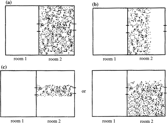

  

  Extent of mixture

  • (a) In Fig. 3.7a, pollutant is fully mixed in the whole room (this is the common case for the buffer room).

  • (b) In Fig. 3.7b, pollutant is distributed in part of the room, but it does not reach the exit of Room 2 (For Room 3 without buffer room belongs to this case).

  • (c) In Fig. 3.7c, pollutant is also distributed in part of the room, but it also reaches the exit of Room 2 (When the room is spacious with shallow depth, this situation may appear).

How is the pollutant distributed, i.e., how is the performance of mixture? It can be expressed with the mixture coefficient α. For small room such as the buffer room, the performance of mixture is good, which is shown in Fig. 3.7a. In this case, α ₂ is set 1. For the case with poor performance of mixture, α ₂ may be 0.2. When there is no air supply in this case, the mixture coefficient could chosen with half at the maximum, i.e., 0.5. On average, it could set 0.35.

Therefore, the resultant concentration can be expressed as follows:

• (1) After the door of Room 1 is closed, the initial pollutant concentration in Room 2 is:

$$N_{20} = \frac{{N_{1} Q_{1} }}{{V_{2} \alpha_{2} }}\,({\text{pc}}/{\text{m}}^{3} )$$

• (2) With the self-purification effect of the air by HEPA filter installed in return air or supply air pipeline, when there is no pollutant particle source in the buffer room and in the atmosphere, the self-purification for this increased concentration can be expressed as follows based on the instantaneous concentration equation [10].

$${\frac{{N_{2t} }}{{N_{20} }} \approx {\text{e}}^{{\frac{ - nt}{60}}} }$$

(3.3)

Next the derivation of this equation will be introduced.

For a room with air supply and air return (exhaust) system and HEPA filter installed in the supply air or return (exhaust) air pipelines, the instantaneous concentration N _t inside the room can be expressed as:

$$N_{t} = \frac{{60G \times 10^{ - 3} + M_{n} (1 - S)(1 - \eta_{n} )}}{{n\left[ {1 - S(1 - \eta_{r} )} \right]}} \times \left\{ {1 - \left[ {1 - \frac{{N_{0} n\left[ {1 - S(1 - \eta_{r} )} \right]}}{{60G \times 10^{ - 3} + M_{n} (1 - S)(1 - \eta_{n} )}}} \right]{\text{e}}^{{\frac{{ - nt\left[ {1 - S(1 - \eta_{r} )} \right]}}{60}}} } \right\}$$

(3.4)

where G is the particle generation rate per volume from occupants and surfaces indoors, pc/(m³ · min); M _n is the atmospheric particle concentration, pc/L; S is the ratio of the return air volume to the supply air volume; η _n is the total efficiency of filters installed on fresh air pipeline; η _r is the total efficiency of filters installed on return air pipeline; N ₀ is the initial concentration indoors.

Let $\frac{{60G \times 10^{ - 3} + M_{n} \left( {1 - S} \right)\left( {1 - \eta_{n} } \right)}}{{n\left[ {1 - S\left( {1 - \eta_{r} } \right)} \right]}} = A$, Eq. (3.4) can be re-written as:

$$N_{t} = A \times \left\{ {1 - \left[ {1 - \frac{{N_{0} }}{A}} \right]{\text{e}}^{{\frac{{ - nt\left[ {1 - S\left( {1 - \eta_{r} } \right)} \right]}}{60}}} } \right\} = A - A{\text{e}}^{{\frac{{ - nt\left[ {1 - S\left( {1 - \eta_{r} } \right)} \right]}}{60}}} + N_{0} {\text{e}}^{{\frac{{ - nt\left[ {1 - S\left( {1 - \eta_{r} } \right)} \right]}}{60}}}$$

For the special case when pathogenic bacteria is released from patients in the isolation ward, it will enter into the buffer room because of the door opening, then it will enter into other rooms. Since there is no bacteria release source in the buffer room and the next following rooms, G = 0. Since there is no such bacteria in the atmosphere, M _n = 0. So A = 0. Therefore, we obtained

$$N_{t} = 0 - 0 + N_{0} {\text{e}}^{{\frac{{ - nt\left[ {1 - S\left( {1 - \eta_{r} } \right)} \right]}}{60}}} = N_{0} {\text{e}}^{{\frac{{ - nt\left[ {1 - S\left( {1 - \eta_{r} } \right)} \right]}}{60}}}$$

Because η _r is the total efficiency of filters installed on return (exhaust) air pipeline, according to Chinese standard, HEPA filters with Type B or higher requirement will be used for this application. The filtration efficiency for bacteria reached more than 99.9999% (refer to Sect. 3.4). So 1 − η _r ≈ 0. Therefore, we obtain:

$$\begin{aligned} N_{t} & = N_{0} {\text{e}}^{{ - {\text{nt}}/60}} \\ \frac{{N_{t} }}{{N_{0} }} & = {\text{e}}^{{\left( { - nt/60} \right)}} \\ \end{aligned}$$

(3.5)

Neither the common cleanroom where there is bacteria generation inside nor the common environment where particles or bacteria exist in the atmosphere is suitable to adopt this equation.

As for Eq. (3.5), when t → ∞, we obtain

$$\frac{{N_{t} }}{{N_{0} }} = 0$$

This means N _t = 0.

In physics, when a certain amount of bacteria enter into the buffer room during the door opening process, it will be self-purified continuously in the buffer room or diluted by the incoming flow and then exhausted. When t → ∞, all the bacteria will be captured by HEPA filter or exhausted outdoors, so that air cleanliness level will be recovered in the buffer room.

When t = ∞, we obtain

$$\frac{{N_{t} }}{{N_{0} }} = 1$$

This means N _t = N ₀. At the moment when bacteria enter into the buffer room, the instantaneous concentration is N ₁, which is the initial concentration of the bacteria in the buffer room.

From the above analysis, before the pollutant enters into Room 3, the pollutant concentration in Room 2 (refer to Fig. 3.8) will be

$$N_{2t} = \frac{{N_{1} Q_{1} }}{{V_{2} \alpha_{2} }}{\text{e}}^{{\left( { - nt/60} \right)}}$$

where t is the self-purification time, min. It starts when the door in Room 1 is closed. It equals to the period for the walking from the door in Room 1 to the door in Room 2 before which is open (the interlock time of the door is included). It is usually between 5 s (~0.1 min) and 30 s (~0.5 min). n is the air change rate, h⁻¹.

Fig. 3.8

Distribution of pollutant after it enters into room 2

• (3) When the door of Room 2 is open and occupant moves from Room 2 to Room 3, the pollutant flux at the gate of Room 3 is shown in Fig. 3.9, which is

  Fig. 3.9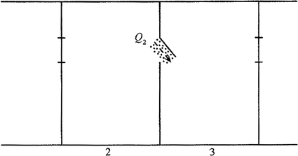

  

  Schematic of pollutant entering into room 3

$$\frac{{N_{1} Q_{1} Q_{2} }}{{V_{2} \alpha_{2} }}{\text{e}}^{{\left( { - nt/60} \right)}} ({\text{pc}})$$

So when the door of Room 2 is closed, the initial concentration of Room 3 becomes

$$N_{30} = \frac{{N_{1} Q_{1} Q_{2} }}{{V_{2} V_{3} \alpha_{2} \alpha_{3} }}{\text{e}}^{{\left( { - nt/60} \right)}}$$

After Room 3 is self-purified, the concentration of the airflow entering into Room 4 becomes

$$N_{3t} = \frac{{N_{1} Q_{1} Q_{2} }}{{V_{2} V_{3} \alpha_{2} \alpha_{3} }}\left[ {{\text{e}}^{{\left( { - nt/60} \right)}} } \right]^{2} ({\text{pc}}/{\text{m}}^{3} )$$

For Room 2, n is big and t is small. While for Room 3, n is small and t is big. For the simplification of assumption in calculation, values of nt are assumed the same, which is shown in Fig. 3.10.

Fig. 3.10

Distribution of pollutant after it enters into room 3

• (4) At the moment when the door of Room 3 is open, the pollutant flux at the gate of Room 4 (buffer room) is shown in Fig. 3.11, which is

  Fig. 3.11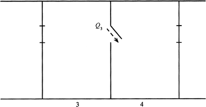

  

  Schematic of pollutant entering into room 4

$$\frac{{N_{1} Q_{1} Q_{2} Q_{3} }}{{V_{2} V_{3} V_{4} \alpha_{2} \alpha_{3} \alpha_{4} }}\left[ {{\text{e}}^{{\left( { - nt/60} \right)}} } \right]^{2}$$

• (5) With the same analysis method for (2), after the pollutant is fully mixed in Room 4, the concentration in Room 4 before the pollutant enters into Room 5, which is shown in Fig. 3.12, becomes

  Fig. 3.12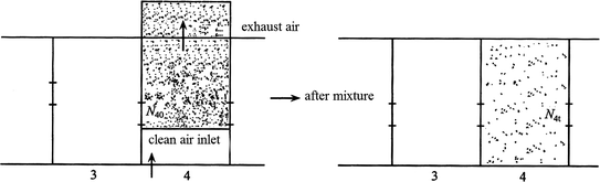

  

  Distribution of pollutant after it enters into room 4

$$N_{4t} = \frac{{N_{1} Q_{1} Q_{2} Q_{3} }}{{V_{2} V_{3} V_{4} \alpha_{2} \alpha_{3} \alpha_{4} }}{\left[ {{\text{e}}^{{\left( { - nt/60} \right)}} } \right]^{3} }({\text{pc}}/{\text{m}}^{3} )$$

• (6) When the pollutant enters into Room 5 from Room 4, the pollutant flux at the gate of Room 5 becomes

$$\frac{{N_{1} Q_{1} Q_{2} Q_{3} Q_{4} }}{{V_{2} V_{3} V_{4} \alpha_{2} \alpha_{3} \alpha_{4} }}\left[ {{\text{e}}^{{\left( { - nt/60} \right)}} } \right]^{3}$$

After the door of Room 4 is closed, the initial concentration of Room 5 (refer to Fig. 3.13) becomes

$$N_{50} = \frac{{N_{1} Q_{1} Q_{2} Q_{3} Q_{4} }}{{V_{2} V_{3} V_{4} V_{5} \alpha_{2} \alpha_{3} \alpha_{4} \alpha_{5} }}\left[ {{\text{e}}^{{\left( { - nt/60} \right)}} } \right]^{3} ({\text{pc}}/{\text{m}}^{3} )$$

Fig. 3.13

Distribution of pollutant after it enters into room 5

3.2.2 Isolation Coefficient of Buffer Room

• 1. Isolation coefficient

  Isolation coefficient is the ratio of the initial concentration in the isolation ward to the induced pollutant concentration in the third room by opening of two doors when the buffer room is set. The larger the total isolation coefficient is, the stronger the prevention ability is. It represents the enhancement ratio of the total prevention ability with buffer room to that without buffer room, which is labeled with β.

Suppose α ₂ = α ₃ = α ₄ = α ₅ = α for Three-Room-One-Buffer scheme, we obtain

$${\beta_{3 \cdot 1} = \frac{{N_{1} }}{{N_{30} }} = \frac{{V_{2} V_{3} \alpha^{2} }}{{Q_{1} Q_{2} \left[ {{\text{e}}^{{\left( { - nt/60} \right)}} } \right]}}}$$

(3.6)

When it is the same assumption for Five-Room-Two-Buffer scheme, we obtain

$${\beta_{5 \cdot 2} = \frac{{N_{1} }}{{N_{50} }} = \frac{{V_{2} V_{3} V_{4} V_{5} \alpha^{4} }}{{Q_{1} Q_{2} Q_{3} Q_{4} \left[ {{\text{e}}^{{\left( { - nt/60} \right)}} } \right]^{3} }}}$$

(3.7)

With the same amount Q (m³) of incoming flow, suppose the number of the buffer rooms is m and the total number of the rooms is k. Volumes of two isolation wards are usually the same, i.e., V ₃ = V ₅ = V, m³. Volumes of two buffer rooms are also usually the same, i.e., V ₂ = V ₄, m³. Suppose the parameter X represents the ratio of the volumes between the isolation ward and the buffer room, we obtain the following general formula.

$${\beta_{k \cdot m} = \frac{{V^{{\left( {k - 1} \right)}} \alpha^{{\left( {k - 1} \right)}} }}{{X^{m} Q^{{\left( {k - 1} \right)}} \left[ {{\text{e}}^{{\left( { - nt/60} \right)}} } \right]^{{\left( {k - 2} \right)}} }}}$$

(3.8)

• 2. Example

Calculation of the entrainment airflow Q from one room to the other can be performed as follows. Since the flow rate induced by the pressure difference 5 Pa is less than 0.05 m³/s, the counteracting effect of the flow rate by the pressure difference less than 5 Pa can be ignored.

From Table 2.11, the flow rate Q of the convection by door opening with Δt = 1 °C within 2 s is 0.44 m³.

From Sect. 2.2.5, the maximum flow rate Q of the entrainment flow during the door opening process is 0.9 m³.

The flow rate of the entrainment flow by occupant movement within 2 s is 0.28 m³.

Therefore, the total flow rate Q is ΣQ = 1.62 m³. (In literatures [7–9], it was 1.52 m³.)

Suppose nt = 6. Since in the buffer room n is very large, we can assume α ₂ = 1. In Room 3 the performance of the air change with air cleaning technique is good, but the value of n is smaller than that in the buffer room. We can assume α ₃ = 0.8. On average α = 0.9. Suppose the volume of the isolation ward is 25 m³ and X = 5, we obtain

$$\begin{array}{*{20}l} {\beta_{3 \cdot 1} = \frac{{25^{2} \times 0.9^{2} }}{{5 \times 1.62^{2} \times 0.9}} = 42.9} \hfill \\ {\beta_{5 \cdot 2} = \frac{{25^{4} \times 0.9^{4} }}{{5^{2} \times 1.62^{4} \times 0.9^{3} }} = 2042} \hfill \\ \end{array}$$

When Room 4 is the buffer room with positive pressure, we assume that the relative pressure difference between Room 4 and the exterior room is ΔP = +5 Pa. When the non-air-tight door is used, the pressurized outward flow rate Q ₄ is

$$Q_{4} = 1.62 + 0.08 = 1.7\,{\text{m}}^{3}$$

$${\beta_{5 \cdot 2} = \frac{{25^{4} \times 0.9^{4} }}{{5^{2} \times 1.62^{3} \times 1.7 \times 0.9^{3} }} = 1943}$$

It is shown that the influence of Room 4, whether it is the negative or the positive pressure buffer room, on the result is not large.

The aforementioned isolation coefficients are related to some prescribed parameters such as the size of the door opening, the period of entrainment by occupant, and the induced flow rate. Therefore only the relationship of the order of the magnitude is reflected in the result. Please do not focus on the specific value.

3.2.3 Influencing Factors for Performance of Buffer Room

• 1. Air change rate

The size of the buffer room is very small. Even when the air change rate reaches 60 h⁻¹, the corresponding flow rate is only 300 m³/h, which is inconsiderable. Therefore air must be supplied into the buffer room.

For the common range of the air change rate in the buffer room, the influence of the air change rate on the isolation performance is not large.

Figure 3.14 shows the influence of the air change rate on the self-purification of the particle concentration (the background concentration is not included) entering into the buffer room, when the air change rate is within the common range [9].

Fig. 3.14

Influence of the air change rate on the self-purification of the particle concentration

After the door is closed, it usually takes 0.1 min to walk to the door of the other side. In Eq. (3.5), e^−nt/60 = N _t/N ₀. It is shown from Fig. 3.14 that the value with 120 h⁻¹ is less than that with 60 h⁻¹ by about 10%, and the influence on β _3·1 is slightly more than 10%.

Table 3.3 illustrates the influence of the air change rate on the isolation coefficient. It is shown that when the air change rate increases by one time, the isolation performance only increases by more than 10%.

Table 3.3 Influence of the air change rate on the isolation coefficient

Of course, when n reaches 1200 h⁻¹, the performance will be improved obviously. However, this is impractical and unrealistic.

• 2. Volume

The larger the volume of the buffer room is, the better the isolation performance is.

From the general formula mentioned above, with the given air change rate, when the volume of the buffer room is larger and when x is smaller, the isolation performance will be better. But when the volume is large, the mixture performance within a certain period will be poor, which means α will be smaller. When the reduction rate of α is not proportional to the increase rate of x, the total isolation performance will improve more. Considering the feasibility for the layout, the volume of the buffer room should not be smaller than 2–3 m².

• 3. Self-purification time

The more the time it takes for occupant to walk through the buffer room, or the more the time it is set for self-lock, the better the isolation performance is.

It is much economic and simpler to increase the self-purification time than to increase the air change rate. When t increases from 6 to 12 s, it is relative easy. But it is equivalent to the increase of the air change rate by one time. Of course, the time for self-lock should not be too long, which is usually within 30 s. Therefore, when serious condition of pollution occurs, the time to open the other door should be delayed, or the time of self-lock should be prolonged to 30 s. Compare with the condition of 6 s, for the air change rate 60 h⁻¹ as shown in Fig. 3.28, the value of e^−nt/60 decreases from 0.9 for the self-lock time 6 s to 0.6 for the self-lock time 30 s. The value of β _3·1 will increase by 1.5 times, and the value of β _5·2 will increase by (1.5)³ times. The total isolation coefficient will be increased as follows:

$$\begin{array}{*{20}l} {\beta_{ 3\cdot 1} {\text{will}}\,{\text{increase}}\,{\text{from}}\, 4 2. 9\,{\text{to}}\, 6 4. 4} \hfill \\ {\beta_{ 5\cdot 2} {\text{will}}\,{\text{increase}}\,{\text{from}}\, 20 4 2\,{\text{to}}\, 6 8 9 2} \hfill \\ \end{array}$$

• 4. Conclusion

From the above-mentioned points 2 and 3, we could not obtain the conclusion that the smaller the buffer room is, the better the isolation performance will be. With the given air change rate, the volume of the buffer room exerts no influence on the air change rate. But when the buffer room becomes small, the value of x in Eq. (3.7) will become large, and the isolation performance will be poor. When the air supply rate is fixed, with the decrease of the volume of the buffer room, the air change rate will become large, and the isolation performance depends on the relative influences on x and n. Even when the isolation performance increases, in essence it is caused by the increase of the air change rate. It should be noted that if the buffer room is as small as half step between two doors, the value of t may be smaller than 6 s by 50%. In this case, the loss outweighs the gain for improving the isolation performance.

3.2.4 Experimental Validation

• 1. Experimental scheme

  • (1) Microbial experiment

In the project entitle with “Research on isolation performance of the isolation ward”, studies on performance of the buffer room was carried out in Institute of Building Environment and Energy, China Academy of Building Research, Beijing, China. Microbial experiment was performed in a simulated isolation ward, where the aforementioned experiment on the pressure difference was performed. Figure 3.15 shows the appearance of the isolation ward. Figure 3.16 shows the preparatory work performed in the ward. Figure 3.17 illustrates the layout of the ward. Parameters in the experiment are shown in Table 3.4.

Fig. 3.15

Appearance of the isolation ward

Fig. 3.16

The preparatory work performed in the ward

Fig. 3.17

Layout of the simulated isolation ward (in the figure, the bathroom did not work. There is no supply air and exhaust air. If the bathroom were real, the door of the bathroom should be open towards the ward inside)

Table 3.4 Related parameters for determining the isolation coefficient in the buffer room with microbial experiment

Figure 3.18 shows the bacteria solution atomization system. Figure 3.19 shows the simulated bacteria generation condition at the mouth.

Fig. 3.18

Schematic of the bacteria solution atomization system

Fig. 3.19

Simulated bacteria generation condition at the mouth

In order to check the function of the buffer room, occupant was required to move outwardly through the door by opening and closing the door for one time (about 2 s).

The type of the bacteria generated is the Bacillus atrophaeus (formerly Bacillus subtilis var. niger) with the strain number ATCC: 15442; 1.3343. It was provided by Biological Resource Center, Institute of Microbiology Chinese Academy of Sciences (IMCAS-BRC).

There are different opinions in literatures about the naked size of the bacteria, which includes 0.5, 0.8, 1 and 1.5 μm. According to the data in literature [11] published in 2003, the linear length and the width of this kind of Bacillus subtilis are 1 and 0.5 μm, respectively. But according to the SEM figure of this paper (which are shown in Figs. 3.20 and 3.21), the linear length for most of the Bacillus subtilis is about 1.2 μm, and a few are smaller than 0.5 μm. As for whether the size of the spores generated in our experiment was the same as that in the published literatures, validation was not performed.

Fig. 3.20

SEM figure of the Bacillus atrophaeus (amplification ratio 1700)

Fig. 3.21

Enlarged SEM figure of the Bacillus atrophaeus (amplification ratio 13500)

After being cultured to be colony forming unit, the color of this kind of bacteria becomes light yellow to red, which is rare for the hybrid strain (including Bacillus subtilis) in atmosphere. So we could consider the background of this kind of bacteria was zero. Error could be avoided. They are easily discovered. The concentration of the bacteria solution, the quantity of the liquid atomized, and the period used for atomization of the liquid should be controlled, so that the bacteria concentration was not too high to be counted in the isolation ward. At the same time, those bacteria passing through the buffer room can be sampled in exterior room, so that the isolation coefficient could be calculated.

Therefore, according to the trial experiment, the bacteria solution concentration was set 10¹⁰–10¹¹ pc/mL. In practice the bacteria solution concentration reached 8 × 10¹⁰ pc/mL. The bacteria solution concentration was determined by the gradual dilution method with the dilution ratio 10.

According to the microbiological experiment method specified in foreign standard, the quantity of the solution atomized should be between 5 and 10 mL. The quantity of air flow rate for generation of bacteria should be 17 L/min. The period for generation of bacteria should be 30 min.

Based on experience, the generated liquid droplet by the atomizer was between 1 and 5 μm. The pressure for atomization was 1 kg/cm².

Bacteria were sampled with the sedimentation method.

The petri dishes should be placed on the floor and near the gate. The measurement points are shown in Fig. 3.22.

Fig. 3.22

Layout of five sampling points on the floor (the direction of the door is illustrated in Fig. 7.15)

• (2) Experiment with atmospheric dust

Table 3.5 shows the experiment parameters.

Table 3.5 Related parameters for experiment on isolation coefficient of buffer room with atmospheric dust

All fresh air was supplied into the isolation ward when the fresh air did not pass through HEPA filter. When the indoor concentration was close to that of the atmospheric dust outdoors, the indoor concentration was measured. The self-purification process was turned on in the buffer room. Measurement was performed in the buffer room to determine if the air cleanliness level ISO 6 has been arrived.

Then the opening and closing of doors were completed. The concentration in the buffer room was measured immediately. The particles entering into the buffer room were considered as microbes. Measurement was performed every 1 min. Three to four readings were recorded. The concentration in the isolation ward was monitored until it reached stable.

• (3) Experiment with temperature difference

Table 3.6 shows the experiment with the temperature difference. For detailed information about the method, please refer to literature [12].

Table 3.6 Conditions in the experiment with the temperature difference

• 2. Experimental results

  • (1) Microbiology method [11, 13]

Figure 3.23 shows the results on No. 5 microbial sampling point in the isolation ward.

Fig. 3.23

Figure of the sedimentation bacteria in the ward

Figure 3.24 shows the results on No. 5 microbial sampling point in the buffer room.

Fig. 3.24

Figure of the sedimentation bacteria in the buffer room

Figure 3.25 shows the results on No. 5 microbial sampling point in the exterior room.

Fig. 3.25

Figure of the sedimentation bacteria in the exterior room

In these figures, the white colony was cultured with the hybrid strain in atmosphere.

It should be noted that only clear figures are presented. Results on No. 5 microbial sampling point in various rooms are relative clear. They cannot be used to obtain the isolation performance exactly, but they can be applied to show the trend of the isolation performance.

Tables 3.7 and 3.8 show the measured data with Scheme 1 and Scheme 2, respectively. In Scheme 1, there is pressure difference and small temperature difference. In Scheme 2, there is no pressure difference and small temperature difference.

Table 3.7 Experimental result on CFU of isolation performance for three-room-one-buffer with pressure difference (−5 Pa) and small temperature difference

Table 3.8 Experimental result on CFU of isolation performance for three-room-one-buffer with no pressure difference (0 Pa) and small temperature difference

According to the above measured data, the isolation coefficients can be obtained as follows.

For Scheme 1 with pressure difference and small temperature difference,

$${\beta_{3 \cdot 1} = \frac{817.8}{40.8} = 20.04}$$

For Scheme 2 with no pressure difference and small temperature difference,

$$\begin{array}{*{20}c} {\beta_{3 \cdot 1} = \frac{752}{42} = 17.9} \\ {\overline{{\beta_{3 \cdot 1} }} = 19} \\ \end{array}$$

• (2) Experimental method with atmospheric dust [14]

The isolation performance with atmospheric dust is obtained through proceeding of data in Table 4.4, which is shown in Table 3.9.

Table 3.9 Experimental result on isolation coefficient for two-room-one-buffer (one isolation ward and one buffer room) with atmospheric dust

• (3) Experimental method with temperature difference

It has been shown in Chapter 2.

• (4) Experimental method with artificial dust

From the data provided in literature [15], the isolation performance with artificial dust for the scheme with one operating room and the other buffer corridor is obtained, which is shown in Table 3.10.

Table 3.10 Experimental result on isolation coefficient for two-room-one-buffer (one operating room and one buffer corridor) with atmospheric dust

• 3. Analysis

• (1) Comparison between theoretical analysis and experimental result

Now the isolation performance with the microbiology method will be analyzed. In the buffer room, there is no exhaust air. The air supply volume can only provide the extremely small amount to maintain the pressure drop across the gap. Therefore, the mixing performance in the buffer room is relatively poor. α ₂ should be smaller than 1, which could be set 0.84. There is no ventilation in the exterior room. According to the analysis in previous section, α ₃ could be set 0.35.

For the scheme with no pressure difference and small temperature difference, the flow rate of air passing through one room to the other room should be as follows. The temperature difference between the buffer room and the exterior room was ∆t = 1 °C, so the total air exchange rate was Q = 1.62 m³. The temperature difference between the isolation ward and the buffer room was ∆t = 2 °C, so the total air exchange rate was Q = 1.8 m³. According to Table 3.4, we know

$${X = \frac{27.6}{6.25} = 4.42}$$

Since in fact there was only air supply with n < 60 and the sedimentation samplings were performed simultaneously in the isolation ward and the buffer room, the influence of the time could be ignored. When t = 2 s, nt < 6 and e^(−nt/60) ≈ 1. Therefore, in theory we obtained

$${\beta_{3 \cdot 1} = \frac{{27.6^{2} \times 0.85 \times 0.35}}{4.42 \times 1.62 \times 1.8 \times 1} = 17.6}$$

The theoretical value is quite close to the measured data which is β _3·1 = 17.9.

For the scheme with pressure difference and small temperature difference, when the flow rate (in 2 s) 0.082 m³ by negative pressure is counteracted, in theory we obtain β _3·1 = 18.5. It is also close to the measured value 20.04.

• (2) By experiments on isolation coefficient with the above-mentioned microbiology method and the experimental method with temperature difference, the isolation coefficients with the microbiology method and the temperature difference method are much smaller than that with the atmospheric dust in the scheme with one isolation ward and one buffer room. The experimental value of the isolation coefficient with atmospheric dust is much larger than the theoretical value. The reason is the self-purification time, which will be analyzed as follows.

The theoretical isolation coefficient is defined by Eq. (3.9), which only considers the entrance of “exterior particles” from the isolation ward to the buffer room.

$${\beta_{2 \cdot 1} = \frac{{N_{1} }}{{N_{2t} }} = \frac{{N_{1} }}{{\frac{{N_{1} Q_{1} }}{{V_{2} \alpha_{2} }}{\text{e}}^{ - nt/60} }} = \frac{{V_{2} \alpha_{2} }}{{Q_{1} {\text{e}}^{ - nt/60} }}}$$

(3.9)

For the data in Table 3.4, the related parameters are as follows.

V ₂ = 6.25 m³

α ₂ = 1 (with exhaust air)

Q ₂ = 1.62 m³/s

n = 112.5 h⁻¹

The maximum value for the pressure difference 0 Pa appears at 1 min (which is shown in Table 3.7), so t = 1 and we obtain

e^−nt/60 = 0.153

Therefore, for the pressure difference 0 Pa, the isolation coefficient is

$${\beta_{2 \cdot 1} = \frac{6.25 \times 1}{1.62 \times 0.153} = 25.2}$$

The theoretical value 25.2 under the real situation is very close to the average measured data 21.7 shown in Table 3.7.

The maximum value for the pressure difference -30 Pa also appears at 1 min, so t = 1. But for the case with large pressure difference, the flow rate by the negative pressure should be counteracted. From Table 2.1, Q ≠ 1.62. Since the air velocity through the door gate is 0.112 m/s, with the area of the door we obtain the flow rate 0.22 m³/s. So Q = 1.4. Therefore, for the pressure difference −30 Pa, we obtain the isolation coefficient

$${\beta_{2 \cdot 1} = \frac{6.25 \times 1}{1.4 \times 0.153} = 29.2}$$

It is very close to the experimental data 40.

The maximum value for the pressure difference −31 Pa also appears at 2 min, so t = 2 and we obtaine^−nt/60 = 0.025

Therefore, for the pressure difference −31 Pa, the isolation coefficient is

$${\beta_{2 \cdot 1} = \frac{6.25 \times 1}{1.4 \times 0.025} = 178.6}$$

The theoretical value 178.6 under the real situation is far from the average measured data 37. The reason may be that for the timing of the optical particle counter, when the end of the reading was 2 min, which may be in fact just passing through 1 min. But it was recorded in the region of 2 min. When 1 min was used for calculation, the theoretical value β _2·1 became 29.2, which is close to the measured data 37.

In literature [16], the experimental data was also calculated with Eq. (3.9) by the Japanese scholar, i.e.,

$${\beta_{2 \cdot 1} = \frac{{V_{2} \alpha_{2} }}{{Q_{1} {\text{e}}^{ - nt/60} }}}$$

where V ₂ is the volume of the isolation corridor, which could set 13 m³.

α ₂ is the coefficient, which could set 1 for the buffer room where air is supplied and exhausted.

Q ₁ is the flow rate. The size of the door is the same as that of the previous case. The time for the previous case is 2 s, but in this case it is 1.6 s. When people arrive at the door, they began to open and close the door. The average time of this process for ten people was obtained. The average flow rate obtained was 1.3 m³ (not 1.62 m³).

n is the air change rate, which is 260/13 = 20 h⁻¹.

t is the first minute when the maximum concentration on the reading of the optical particle counter.

Therefore, for the pressure difference 0 Pa, the isolation coefficient is

$${\beta_{2 \cdot 1} = \frac{13 \times 1}{1.3 \times 0.72} = 14}$$

For the case with the pressure difference -30 Pa, the flow rate by the negative pressure should be counteracted. Q = 1.1 m³. The theoretical value β _2·1 became 16.4.

• (3) During the experimental method with temperature difference, the air supply rate in the buffer room is 379 m³/h and n = 60.64 h⁻¹. Since there is air supply and air exhaust with large air change rate, α = 1.

Based on past calculation data, the flow rates Q under different temperature difference conditions is: 1.38 m³ for 0.2 °C, 1.92 m³ for 3 °C, and 2.14 m³ for 5 °C.

In the previous 2 min, e^−nt/60 = 0.134. Theoretical and experimental data for the isolation coefficient are shown in Table 3.11.

Table 3.11 Theoretical and experimental data for the isolation coefficient of the outwardly opening door during the experiment with the temperature difference

It is shown that the calculation result in theory could be used to estimate the actual isolation performance on average.

Both the theoretical and measured data are summarized in Table 3.12. The difference between the theoretical and measured data is large only for the method with atmospheric dust. This is related to the explanation of the original data. But for other methods, the difference is very small. When some parameter is not accurate enough, the influence on the result will be very large. For example, when the error for determining the value of t is several seconds, this influence will appear. Therefore, there is still relative reference value in the theoretical equation.

Table 3.12 Comparison of the theoretical and measured isolation coefficients

• (4) Influence of the pressure difference on the isolation performance

Based on the aforementioned experimental data, it is shown that the influence of the pressure difference on the isolation performance is not large. This is because the counteracting flow rate by the negative pressure difference on the outward leakage flow rate is very small. Results are shown in Table 3.13.

Table 3.13 Influence of the pressure difference on the isolation performance

It takes too much effort to create the pressure difference −30 Pa, compared with the situation with the pressure difference 0 Pa. However, the amplification magnitude for the increase of the isolation coefficient is not too much.

Besides under the condition with the pressure difference −30 Pa, when there is temperature difference, the pollutant cannot be prevented from leakage outwardly during the opening process of the door. From Table 2.3, the quantity of the leakage flow rate still reached more than one fifth of the original concentration. Therefore, the cost-effective performance to adopt the pressure difference −30 Pa is almost the same as that of the situation with −5 Pa.

In short, it is not reasonable and safe to pursue the isolation performance by increasing the pressure difference. When the pressure difference increases from 0 to −30 Pa, the isolation performance is increased by more than one time. However, when one buffer room is added, the isolation coefficient β _3·1 will be increased by a dozen times.

3.2.5 Door of Buffer Room

There are two doors for the buffer room. One is the door adjacent to the isolation ward, which can also be called the door of the ward. The other is the door for entrance into the interior corridor. For the purpose of convenience, the former door is called the inner door of the buffer room, and the latter is called the outer door of the buffer room.

As mentioned before, the extent of the air-proof for the inner door has no effect on the outward leakage of air flow. However, there are still differences for different kinds of the doors. From Fig. 2.6 and Table 2.8, the performance of the outwardly opening door is poorer than that of the inwardly opening door which has worse performance than the sliding door.

The air velocity of the counter current has been introduced before. Figure 3.26 illustrates the air velocities of the counter current during the opening and closing of three different door under different pressure difference conditions. In the figure, the component of −x means the direction from indoors towards outdoors, and the component of +y means the direction from the heel post of the door towards the door handle, which are shown in Fig. 3.27. Since the air velocity of the y component during the closing of the door is larger than that during the opening of the door, the air velocity of the +y component during the closing of the door is presented in the figure [15].

Fig. 3.26

Relationship between the air velocities of the counter current during the opening and closing of the door and the pressure difference

Fig. 3.27

Schematic diagram of the air velocity components for the counter current

In this experiment, the air velocity of the counter current reached more than 1 m/s, which is obviously larger than the measured values by American scholar and our study. In this experiment, the air velocity is the one during the pushing process of the door, while in our study the air velocity was measured after the door was open. This may be the reason for the difference.

From the figure, it is shown that:

• (1) The magnitude of the air velocity for the counter current is: outwardly opening door > inwardly opening door > sliding door. This can be used to explain the sequence for the relationship between the particle number transmitted during the opening of the door and the type of the door shown in Fig. 2.6.

• (2) The air velocity of the counter current is not related to the pressure difference. This means the air velocity of the counter current for ΔP = 0 Pa is close to that for ΔP = 30 Pa. It even beyonds the imagination that for the inwardly opening door, the air velocity of ΔP = 0 Pa is the maximum while that for ΔP = 30 Pa is the minimum.

From the aforementioned analysis, with the suitable size of the buffer room, the sliding door could be adopted as the inner door, and the outwardly opening door could be utilized as the outer door. For the ward with negative pressure, the outwardly opening door can be used only. The problem of increasing the air-proof performance cannot be considered. The door with common air-proof performance is fine, except that the wooden material is not used.

3.3 Airflow Isolation in Mainstream Area

3.3.1 Concept of Mainstream Area

Medical personnel for ward round or operation near the sickbed will face the pollutant source directly. During the talking, coughing and sneezing processes of patients, it will pose a threat to the medical personnel. The range hood introduced in Chapter One has been denied by practice. There is a certain effect of prevention for wearing common masks. As for the designer of the isolation ward, how can we reduce the infectious risk of the medical personnel under the dynamic condition of the operation with the current air cleaning system?

For protecting the medical personnel, CDC manual in U.S.A. proposed that clean air should be passing through the working area of the medical personnel. No only CDC emphasized this point, but also other related literatures has mentioned it. But one fact has been ignored, which is shown in Fig. 3.28. When clean air is supplied from the back of the people, negative pressure area will be formed in the front breathing zone of the people, which has no protective effect and is harmful.

Fig. 3.28

Negative pressure area formed in the front zone of the people

Therefore, in the concept of dynamic isolation theory, the measures to utilize the mainstream area are proposed, which has been validated effectively.

In 1979, the concept of the mainstream area was proposed by author [3], which is shown in Fig. 3.29. The region of the downward supply air below the air supply outlet can be termed as the mainstream area. In this area, the air cleanliness level is the best and the ability to exhaust pollution is the best. At the upper region of the mainstream area, some of the surrounding air will be sucked in, which will be diluted and then exhausted together from the lower part of the room.

Fig. 3.29

Schematic diagram of the mainstream area

When air is supplied and then exhausted as shown in Fig. 3.29, the average indoor concentration is:

$${N_{v} = N_{s} + \psi \frac{{60G \times 10^{ - 3} }}{n}}$$

where N _v is the average indoor concentration; N _s is the concentration of the supplied air; G is the bacteria generation rate per unit volume; n is the air change rate; ψ is the non-uniform distribution coefficient (please refer to Table 3.14).

Table 3.14 Non-uniform distribution coefficient ψ

The parameter ψ can be calculated as follows.

$${\psi = \left( {\frac{1}{\varphi } - \frac{\beta }{\varphi } + \frac{\beta }{1 + \varphi }} \right) \times \left( {\varphi + \frac{{V_{b} }}{V}} \right)}$$

(3.10)

where φ is the carrier ratio of the airflow. The value φ becomes 1.5, 1.4, 1.3, 0.65, 0.3 and 0.2 when the area corresponding to each air supply unit with air filter inside on the ceiling is ≥7, ≥5, ≥3, ≥2.5, ≥2 and ≥1 m², respectively. β is the ratio of the particle generation rate in the mainstream area to that in the whole room; V is the room volume; V _b is the volume of the vortex area.

For the isolation ward with single patient and with the air change rate n ≈ 10⁻¹, the value of ψ is 1.5 based on Table 3.14. In this case, the average indoor concentration is:

$${N_{v} = 1.5 \times \left( {N_{s} + \frac{{60G \times 10^{ - 3} }}{n}} \right)}$$

3.3.2 Function of Mainstream Area

The mainstream area was proposed to protect the medical personnel. Air supply outlet is placed on top of the positions where medical personnel performed the ward round and operation near the sickbed of the patient, which is shown in Fig. 3.30.

Fig. 3.30

Schematic of the medical personnel near the sickbed under the protection of the mainstream area

If there is no particle generation source in the mainstream area as shown in Fig. 3.30, β = 0. The area of the room is larger than 10 m². If there is only one air supply outlet, the parameter is φ = 1.5.

Therefore, the non-uniform distribution coefficient in the mainstream area becomes

$$\psi = 1 - \frac{\beta }{1 + \varphi } = 1 - \frac{0}{1 + 1.5} = 1$$

The average concentration in the mainstream area is

$${N_{a} = N_{s} + \frac{{60G \times 10^{ - 3} }}{n}}$$

Therefore, based on the expressions of the concentration in the mainstream area and the average indoor concentration N _v, we obtain

$$N_{\text{a}} = 0.67N_{\text{v}}$$

This means that the pollutant concentration in the mainstream area where the medical personnel stay and face as the breathing zone is about 2/3 of the average indoor concentration. This is much less than that in the vortex area.

In other words, when the medical personnel stays in any place indoors (except the breathing area in front of the patient), the pollutant concentration could be considered as the average indoor concentration N _v. But when the medical personnel stay inside the mainstream area, the pollutant concentration can be reduced to 2/3 of N _v.

Compared with the concentration in the breathing zone of the patient, the concentration in the mainstream area is much smaller. This is because the pollutant entering into the mainstream area only accounts for a small proportion, which is further diluted by the supplied air in the mainstream area. Therefore, the concentration of the mainstream area is much less than 2/3 of the average indoor concentration.

Because in the ward, patient stays inside alone, or stays with other patients who carry the same kind of disease. They are already adapted to this habitat environment. The average indoor concentration is not too important for them. However, for the medical personnel, although they walk around in the ward, they will usually stay for a long period besides the sickbed. Because they are healthy people, they are sensitive to the indoor pollutant. Therefore, the pollutant concentration in this region should be as small as possible.

This is the reason why the air supply outlet should be placed above the side of the sickbed where the medical personnel usually stay. It is aimed to protect the medical personnel through the mainstream area.

Because of such performance of the mainstream area, the mainstream area should be enlarged as much as possible. With the given area of the air filters, the area of the air supply outlet should be increased, as long as the air velocity at the air supply outlet is not small than 0.13 m/s [4]. Otherwise, the performance will be opposite.

3.4 Application of Self-circulation Air Through HEPA Filter

3.4.1 Application Principle of Circulation Air

From Chap. 2, we know that it is a misunderstanding that circulation air is not allowed for usage. But for the application of circulation air in the concept of the dynamic isolation, there are several principles:

• (1) The circulation air does not mean the circulation of the return air in the central system for different rooms. It is the self-circulation for the air in each room.

• (2) There must be a proportion of circulation air to be exhausted outdoors, so that negative pressure can be kept indoors. On the exhaust air outlet, HEPA filter must be installed.

• (3) The exhaust air outlet and the return air outlet can be combined to be one apparatus. HEPA filter could be shared for both the exhaust air and the return air.

• (4) The exhaust air outlet and the return air outlet are not required to be free of leakage.

3.4.2 Function of HEPA Filter

• 1. Common disinfection methods

  • (1) Features of common disinfection method

    In order to deal with pollution and infection in hospitals, pipeline cleaning and spraying sanitization were usually adopted in the past. Chemical and physical disinfection methods were utilized indoors. This kind of treatment methods with pollution at first and then control is termed as the passive treatment. It will yield twice the result with half the effort. Besides, it is a method with sequela. It is not a method to control pollution during the whole process. Instead, it only pays attention to pollution control at the beginning and the end.

    In hospitals the objects where disinfection is needed include: occupant, surfaces of object, and air. For occupant, hands need to be disinfected. People needs to take a bath and wear aseptic clothes.

    For surfaces of object, it should be wiped clean. The following methods may be used, which include the disinfection with chemical agent (more than one type must be used), the moist heat sterilization, the dry heat sterilization, the radiation sterilization, the gas sterilization, sterilization with air filtration (when sterilization cannot be performed eventually in the container).

  • (2) Examples of air disinfection method

    Table 3.15 illustrates various methods for air disinfection, where the air disinfection efficiencies were shown in the product catalog, literatures, claim from manufacturer or the test report.

    Table 3.16 illustrates the measured result on electrostatic sterilization equipment performed by experts from Institute of Microbiology and Epidemiology at the Academy of Military Medical Sciences [17].

    Table 3.17 shows the report from Chinese Journal of Nosocomiology [18]. Table 3.18 shows the data from Tianjin University [19] and National Center for Quality Supervision and Test of Building Engineering [20]. Table 3.19 presents the report data by National Center for Quality Supervision and Test of Building Engineering. Table 3.20 provides the data from the thesis at China Academy of Building Research [20]. Table 3.21 shows the data from literature [21]. Table 3.22 presents data from the Academy of Military Medical Sciences [17] and the dissertation at Tongji University [22].

Table 3.15 Various methods for air disinfection

Table 3.16 Bacteria removal efficiency by electrostatic sterilization equipment

Table 3.17 Comparison on sterilization performance of different disinfection methods

Table 3.18 Data from Tianjin University [19]

Table 3.19 Report data by National Center for Quality Supervision and Test of Building Engineering

Table 3.20 The data from the thesis at China Academy of Building Research

Table 3.21 Efficiency of electrostatic air cleaner

Table 3.22 Sterilization efficiency of electrostatic air cleaner

• 2. Features of disinfection method with HEPA filter

  • (1) Whole-process control

    When air cleaning system with HEPA filter is used during the whole operation process indoors, the indoor air environment can be controlled. This is different from “sterilization at the beginning” or “sterilization at the end”.

  • (2) Both dust and bacteria are removed

    By using the principle of physical barrier, air filter can remove dust, as well as microbes (including bacteria and virus). Since microbes are carried by particles, bacteria can be removed during the removing process of dust.

  • (3) No generation of other gradients

    Some sterilization method may generate toxic gases such as nitrogen oxides or ozone. However, air filtration is a pure physical method, which will not generate other gradients.

  • (4) No side effect of generating toxic material

    Some sterilization method may generate radiation, which is harmful to occupant’s health. Some generated electric field or magnetic field has influence on instrument and equipment. Some may promote the mutation of bacteria. For example, this will occur during the UV irradiation. The drug resistance of the bacteria may become very strong.

  • (5) High and complete sterilization efficiency

    For HEPA filter, the sterilization efficiency could reach more than 99.99999%. The sterilization performance is complete. There are no semi-lethal bacteria left, which may revive afterwards. For bacteria suffering UV irradiation, they may revive under the light if they are not killed by irradiation. Bacteria corpse or secretion will not left if HEPA filter is used.

  • (6) Broad-spectrum of sterilization efficiency and easy for selection

    The range of sterilization efficiency for different products is from 10 to 99.999999%, while that of other sterilization methods is very narrow, which is from 70 to 90%.

  • (7) It is not selective for dust and bacteria removal

    The performance of some sterilization method such as the electrostatic method is influenced by the conductivity property of the dust particles. Some sterilization method is selective for the type of bacteria, which means the sensitivity level is different.

    For example, the UV-C ray with wavelength 253.7 nm has different sensitivity levels for various microbes, which is shown in Table 3.23 [23].

    Table 3.23 Sensitivity of various typical microbes for UV ray

  • (8) It is a method to prevent aerosol and airborne microbes from entering into the air ducts.

It is equivalent to the method of preventing the enemy from invading into our country. It is the highest state of war to subdue the enemies without fight. This method will not cause corpses of the bacteria cover the plain. Therefore, it is an active pollution control method, and not the passive method to perform disinfection after bacteria come indoors. It is a green method to build the green hospitals. No new pollution will be generated.

Of course, the main shortcoming of air filter is its relative large pressure drop. But pre-filter or filter for air supply outlet should also be installed for some methods, including the nano-photocatalysis and UV equipment. Air filters with lower pressure drop should be utilized. Related technique and products have been available.

• 1. Classification of air filters

  • (1) Table 3.24 shows the classification of air filters according to national standard GB/T 14295-2008.

    Table 3.24 Performance classification of air filters

  • (2) Classification for HEPA and ULPA filter

    Classifications for HEPA and ULPA filters according to national standard GB/T13554-2008 are shown in Tables 3.25 and 3.26, respectively.

    Table 3.25 Classifications for HEPA and ULPA filters

    Table 3.26 Approximated comparison of several standards for air filters from China and abroad

  • (3) Comparison of classification standards between China and abroad

    The test conditions for air filters in standards from China and abroad are quite different, including the particle source and its diameter. Only approximated instead of quantitative comparison can be performed, which is shown in Fig. 3.26.

3.4.3 Experimental Validation for Application of HEPA Filter with Circulation Air

• 1. Experimental method

  Experiment was performed in the aforementioned simulated isolation ward as shown in Fig. 3.17. Bacteria were released outside of the air filter for exhaust air. The bacterial concentration for spray was 8 × 10⁸ pc/mL.

Leakage may occur on the frame of the air filter as shown in Fig. 3.31, which may not be detected beforehand and then sealed (a leakage-free exhaust air apparatus was invented, which will be introduced in detail later). In order to prevent the spread of aerosol into the room from the bacterial release position at the exhaust (return) air outlet, casing pipe must be used for bacteria generation inside.

Fig. 3.31

Leakage on the frame of air filter for exhaust (return) air

If the frame of air filter is very air-tight, the casing pipe should contact air filter directly, which is shown in Fig. 3.32 [24]. In the figure, Q is the flow rate of the circulation air in the room, m³/h; q ₁ is the air flowrate during the spray, m³/h; q ₂ is the air flowrate sucked into the casing pipe, m³/h; k is the penetration of HEPA filter at the return air outlet, %; C is the bacterial generation rate, pc/h.

Fig. 3.32

Direct contact of casing pipe with air filter

It is obvious that the aerosol concentration in the supply air is kC/Q.

When there is leakage air on the frame of air filter or when the casing pipe does not closely contact the air filter as shown in Fig. 3.33 [24], is there any influence on the measured result?

Fig. 3.33

Leakage air on the frame of air filter and casing pipe

In Fig. 3.33, q ₁ is the air flowrate during the spray, m³/h; q ₂ is the air flowrate sucked into the casing pipe, m³/h; q ₃ is the flowrate of the leakage air, m³/h; Q is the flow rate of exhaust air through air filter, m³/h; k is the penetration of air filter,%; C is the bacterial generation rate, pc/h; Q/X is the flowrate inside the casing pipe (Q/X = q ₁ + q ₂, Q = q ₂ + Q/X), where X is the ratio which is larger than 1.

In this case, the concentration of entering air from return air opening is C/(Q/X), pc/m³. The penetrated aerosol in air is kC/(Q/X). The total quantity of aerosol penetrated is:

$${\frac{kC}{{\frac{Q}{X}}} \cdot \frac{Q}{X}/Q = \frac{kC}{Q}}$$

This means that the concentration is the same as that from the supply air for the case when the casing pipe is required to contact air filter directly and when there is no leakage on frame of air filter. This proves that it is feasible to use casing pipe for bacterial generation.

With the same method, bacterial concentration can be measured below the air supply outlet with the sampling method for planktonic bacteria, which is shown in Fig. 3.34.

Fig. 3.34

Measurement of planktonic bacteria at the air supply outlet

• 2. Experimental results

The measurement condition is shown in Table 3.27 [24]. The measurement results are presented in Table 3.28 [14]. In the table, the measured concentration for the supply air at the air supply outlet is expressed with CFU/petri dish.

Table 3.27 Experimental condition

Table 3.28 Measurement result for filtration efficiency with bacteria

Hourly bacterial generation rate at the return air opening = Bacterial solution concentration per minute × Spray quantity of bacterial solution × 30 min × 2

Bacterial generation concentration at the return air opening = Bacterial generation rate at the return air opening ÷ flow rate of return air

It is shown from Table 3.27 that for HEPA filter B, the filtration efficiency for the spray strain reached 99.99997%. For HEPA filter C, the filtration efficiency for the spray strain reached 99.999997%. Both efficiency of these two kinds of filters are larger than the measured efficiency with atmospheric dust. This is consistent with the aforementioned factor of equivalent diameter of microorganism. Filtration efficiency of HEPA filter C for bacteria is higher than that of HEPA filter B by one order of magnitude. This is also consistent with the relationship of the filtration efficiency with atmospheric dust between two products.

Next quantitative analysis will be performed.

The relationship between different particle diameters is given by empirical equation [25].

$${k_{2} =\frac{{k_{1} }}{{{\text{e}}^{{\left( {d/d_{0.3} } \right)^{2} }} }}}$$

(3.9)

where k ₁ and k ₂ are the penetrations for particle size 0.3 μm and particle size larger than 0.3 μm, respectively; d _0.3 and d are the particle size 0.3 μm and the particle size larger than 0.3 μm, respectively;

From the above experiment shown in Table 3.27 [14], the measured efficiency of HEPA filter B before delivery from factory for atmospheric dust with diameter ≥0.5 μm is 99.999%. From literature [25], the efficiency with atmospheric dust for particle size 0.3 μm can be calculated to be 99.93%, which corresponds to the penetration k = 0.07%. The measured efficiency of HEPA filter C before delivery from factory for atmospheric dust with diameter ≥0.5 μm is 99.99994%. The efficiency with atmospheric dust for particle size 0.3 μm can be calculated to be 99.998%, which corresponds to the penetration k = 0.002%.

From Chap. 5, water component in the sprayed droplet will evaporate quickly during the spray process, but residual solute will be left. Since the size of the sprayed droplet is usually 1–5 μm, the average size is 3 μm. From Chap. 5, the final size of the solute is 0.16 × 3 = 0.48 μm, so it should be added into the size of naked bacteria. Since the size of the spore is about 1 μm, the increase of the linear thickness on the surface can be ignored.

Table 3.29 illustrates the efficiency for spores with different diameters.

Table 3.29 Efficiency for spores with different diameters

Based on the measurement result from Table 3.28, the measured efficiency is within the range of the calculated efficiency for spores with diameter 0.8 and 0.9 μm. From Table 3.24, the concentration at the air supply outlet, when HEPA filter C was applied, was in the order of the natural number magnitude. This means for such high efficiency in experiment, when the bacteria concentration was increased by an order of magnitude, the measured efficiency may become higher.

The above measured result is equivalent with the foreign experimental data in Table 3.30 [26]. The corresponding filtration velocity is only less than a half of the filtration velocity in Table 3.30, so the efficiency value is slightly higher.

Table 3.30 Filtration efficiency of various air filters for serratia marcescens (the bacterial solution concentration for spray is 1.1 × 10⁷ pc/L)

The above efficiency values with the sodium flame method, DOP method and particle counting method are different. For particle counting method, the efficiency for particle size 0.3 μm is different from that for particle size ≥0.5 μm, which could be referred to literature [25].

In short, the theoretical efficiency with actual particle size should be larger than the experimental data. So it is much safe to use experimental data.

It is known that the number of aerosol during coughing could reach more than 3 × 10⁵. When ten times of this concentration, i.e., 3 million bacterial particles, pass through HEPA filter B, only one particle could penetrate. When one hundred times of this concentration, i.e., 30 million bacterial particles, pass through HEPA filter C, only one particle could penetrate.

Therefore, the bacterial concentration in the circulation air through HEPA filtration unit is much smaller than indoor bacterial concentration. For patients staying in a room with such low bacterial concentration for a long time, it is not doubt that the influence of circulation air is little. This means it is feasible to apply HEPA filtration unit in isolation ward.

References

Z. Xu, in Design, Operation and GMP Accreditation on Pharmaceutical Factory, 2nd edn. (Tongji University Press, 2011), pp. 42
Z. Xu, in Design Principle of Isolation Ward (Science Press, Beijing, 2006), pp. 5–18
Z. Xu, in Fundamentals of Air Cleaning Technology, 4th edn. (Science Press, Beijing, 2014) pp. 401
Z. Xu, in Design, Operation and GMP Accreditation on Pharmaceutical Factory, 1st edn. (China Architecture & Building Press, Beijing, 2002) pp. 208
E. Moia, Keypoints of biological isolation facilities, in Proceedings of the 6th China International (Shanghai) Academic Forum & Expo on Cleanroom Technology, 2003, p. 317
T. Zhao, K. Jia, Discussion on the pressure control of BSL-3 laboratory, Build. Sci. no. supplementary issue, pp. 112–115 (2005)
Z. Xu, Y. Zhang, Q. Wang, H. Liu, F. Wen, X. Feng, Isolation principle of isolation wards. J. HV&AC, 36(1), pp. 1–7, 34 (2006)
Z. Xu, Y. Zhang, Q. Wang, F. Wen, H. Liu, L. Zhao, X. Feng, Y. Zhang, R. Wang, W. Niu, Y. Di, X. Yu, X. Yi, Y. Ou, W. Lu, Study on isolation effects of isolation wards (1). J HV&AC 36(3), 1–9 (2006)
Z. Xu, The application of surge chamber of negative pressure isolating room. Chin. Hosp. 10(10), 17–20 (2006)
Z. Xu, in Fundamentals of Air Cleaning Technology and Its Application in Cleanrooms. (Springer Press, 2014), pp. 449–454
J.A. Schmidt, in System and Method of Applying Energetic Ions for Sterilization, Official Gazette of the United States Patent & Trademark Office Patents (2003)
Z. Xu, Y. Zhang, Q. Wang, H. Liu, F. Wen, X. Feng, Y. Zhang, L. Zhao, R. Wang, W. Niu, D. Yao, X. Yu, X. Yi, Y. Ou, W. Lu, Study on isolation effects of isolation wards (3). J. HV&AC 36(5), 1–4 (2006)
L. Zhao, Z. Xu, X. Yu, Q. Wang, Y. Zhang, F. Wen, H. Liu, Y. Di, R. Wang, H. Zhao, Microbiology experimental method for insulation effect of isolation wards. J. HV&AC 37(1), 9–13 (2007)
Y. Zhang, Z. Xu, Q. Wang, H. Liu, F. Wen, L. Zhao, X. Feng, Y. Zhang, R. Wang, W. Niu, Y. Di, H. Zhao, X. Yu, X. Yi, Y. Ou, W. Lu, Experiment on germ filtering efficiency of high efficiency filters on return air inlet in isolation wards. J. HV&AC, 36(8), pp. 95–96 + 112 (2006)
S. Honda, Y. Kita, K. Isono, K. Kashiwase, Y Morikawa, Dynamic characteristics of the door opening and closing operation and transfer of airborne particles in a cleanroom at solid tablet manufacturing factories. Trans. Soc. Heating, Air-Conditioning Sanit. Eng. Japan, 95, pp. 63–71 (2004)
Z. Xu, Y. Zhang, Y. Zhang, Z. Mei, J. Shen, D. Guo, P. Jiang, H. Liu, Mechanism and performance of an air distribution pattern in clean spaces. J. HV&AC 30(3), 1–7 (2000)
H. Yang, “Implication of electrostatic sterilization in air cleaning,” in the 37th Pharmaceutical Preparations Forum & the 4th Pharmaceutical Disinfection and Sterilization Symposium, 2009, pp. 127–128
C. Wu, M. Du, Effects of four kinds of indoor air sterilization method. Chin. J. Nosocomiology 10(6), 403 (2000)
Y. Wang, in Study on Air Sterilization Technique with Dynamic UV Irradiation in Air Duct. (Tianjin University, 2011)
H. Pan, Discussion on applicability of sustained using ultraviolet rays in air conditioned rooms for disinfecting and sterilization: part 6 of the series of research practice of the revision task group of the architectural technical code for hospital clean opera. J. HV&AC, 43(7), pp. 27–29 + 36 (2013)
Z. Xu, Fundamentals of Air Cleaning Technology, 4th edn. (Science Press, Beijing, 2014)
H. Mao, in Study on Improvement of Indoor Air Quality by Application of Electrostatic Air Cleaner. (Tongji University, 2008)
J. Mao, J. Shen, Control concept and practice for the sterilized space. Contam. Control Air-Conditioning Technol. 4, 9–12 (2003)
Z. Xu, Design Principle of Isolation Ward. (Science Press, Beijing, 2006), pp. 149
Z. Xu, in Fundamentals of Air Cleaning Technology and Its Application in Cleanrooms. (Springer Press, 2014, 2014), pp. 205–207
Z. Xu, Fundamentals of Air Cleaning Technology and Its Application in Cleanrooms. (Springer Press, 2014), pp. 499. Fig. 3.1 Schematic diagram of gap
J. Shen, Multi-application isolation ward and its air conditioning technique without condensed water. Build. Energy Environ. 24(3), 22–26 (2005)
Author information
Authors and Affiliations
Corresponding author
Rights and permissions
Copyright information
© 2017 Springer Nature Singapore Pte Ltd.
About this chapter
Cite this chapter
Xu, Z., Zhou, B. (2017). Principle and Technology of Dynamic Isolation. In: Dynamic Isolation Technologies in Negative Pressure Isolation Wards. Springer, Singapore. https://doi.org/10.1007/978-981-10-2923-3_3
Download citation
DOI: https://doi.org/10.1007/978-981-10-2923-3_3
Published:
Publisher Name: Springer, Singapore
Print ISBN: 978-981-10-2922-6
Online ISBN: 978-981-10-2923-3
eBook Packages: EngineeringEngineering (R0)