
Abstract
Traditionally all the macroscopic phenomena observed in nature have been studied via solutions of differential equations (DE) which are described by smooth and continuous curves. This approach works very well for a class of problem like the planetary motion where the orbits are regular geometric objects (namely, ellipse). However, there is a class of problems like the fluid turbulence which involves growth of objects of irregular shape (fractals and multi-fractals, see Chaps. 6 and 9) and cannot be studied via smooth solutions of DE’s.
Access this chapter
Tax calculation will be finalised at checkout
Purchases are for personal use only
Notes
- 1.
The concept of flow here is predicated on the resemblance of the solution trajectories to the paths followed by particles of a flowing fluid. Therefore, the language of fluid mechanics has often been used to visualize a continuous group of motions or mappings.
- 2.
The IVP, on the other hand, is said to be ill-posed if the solution x(t) exists only for an analytic initial condition (1.5) and, even when it does exist, it develops singularities in a finite time.
- 3.
In general, Lipschitz condition is stronger than differentiability.
- 4.
The application of this principle to physical systems can however lead to some difficulties. Because, if the solutions depend sensitively on the initial conditions, then any inexact knowledge of the initial state would make the prediction of the final state difficult (if not impossible).
- 5.
If an eigenvalue λ k is μ k -fold (μ k >1) degenerate, the matrix A cannot be diagonalized. The best one can do in such a situation is to reduce A to a Jordan canonical form; in this form, there is a Jordan block of order, say, μ k ×μ k ,
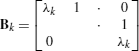
corresponding to eigenvalue λ k . In order to calculate \(e^{t \mathbf{B}_{k}}\), we write Arnol’d (1973),
$$ \mathbf{B}_k = \lambda_k \mathbf{I} + \mathbf{J} $$where,

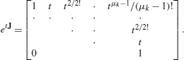
Noting that,
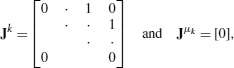
we have,
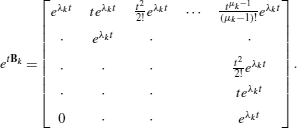
Next, noting that, for two matrices A and B which commute,
$$ e^{\mathbf{A}+\mathbf{B}} = e^\mathbf{A} e^\mathbf{B} $$we have,
- 6.
A homeomorphism is a continuous, one-to-one mapping with a continuous inverse.
- 7.
For a two-dimensional problem, equations (1.81) and (1.82) take the obvious form
$$ \left . \begin{array}{l} x^\prime_1 =f_1(x_1,x_2)\\ x^\prime_2 =\pm x_2 + f_2(x_1,x_2). \end{array} \right\} $$So, the motion on the stable/unstable manifolds is governed by the dominant linear terms while the motion the center manifold is governed by the nonlinear terms in the differential equation.
- 8.
The center is structurally unstable because arbitrarily small perturbations of the system can turn it into a focus.
- 9.
The canonical form for a focus is
$$ x^\prime=y + ax ,\qquad y^\prime= -x + ay. $$If a<0, one has a stable focus, while if a>0, one has an unstable focus. The trajectories are logarithmic spirals of the form
$$ \rho=e^{a\theta},\qquad \rho\equiv\sqrt{x^2+y^2},\qquad \theta\equiv\tan^{-1}(y/x). $$ - 10.
The canonical form for a stable node is
$$ x^\prime= -x,\qquad y^\prime= ay\quad (a < 0) $$while that for an unstable node is
$$ x^\prime= x,\qquad y^\prime= ay\quad(a > 0). $$ - 11.
The canonical form for a saddle point is
$$ x^\prime= x,\qquad y^\prime= -y. $$ - 12.
Such an organization of the phase space by centers (or elliptic points) surrounded by the separatrices meeting at the saddle points (or hyperbolic points) is typical for integrable dynamical systems. Indeed, the representation of the motion of a general integrable two-degree-of freedom system on a Poincaré surface of section looks like a distorted version of the phase-plane portrait of the simple pendulum (see Chap. 5).
- 13.
In a practical situation, there is always difficulty in distinguishing between a periodic solution with a very long period and a genuine non-periodic solution.
- 14.
When there is some damping present in the system, these jump phenomena lead to a dynamic hysteresis effect—the response of the system depends on its past history so that the system responds differently when λ is increased than when λ is decreased.


References
V.I. Arnol’d, Ordinary Differential Equations (MIT Press, Cambridge, 1973)
C. Bender, S.A. Orszag, Advanced Mathematical Methods for Scientists and Engineers (McGraw-Hill, New York, 1978)
J. Guckenheimer, P. Holmes, Nonlinear Oscillations, Dynamical Systems, and Bifurcations of Vector Fields (Springer, Berlin, 1986)
P. Hagedorn, Nonlinear Oscillations (Oxford University Press, London, 1988)
J. Hale, H. Kocák, Dynamics and Bifurcations (Springer, Berlin, 1991)
M. Hirsch, S. Smale, Differential Equations, Dynamical Systems and Linear Algebra (Academic Press, San Diego, 1974)
J.E. Marsden, M. McCracken, The Hopf Bifurcation and Its Applications (Springer, Berlin, 1976)
H.G. Schuster, Deterministic Chaos, 3rd edn. (VCH Verlag, Weinheim, 1995)
R.A. Struble, Nonlinear Differential Equations (McGraw-Hill, New York, 1962)
Author information
Authors and Affiliations
Rights and permissions
Copyright information
© 2014 Springer Science+Business Media Dordrecht
About this chapter
Cite this chapter
Shivamoggi, B.K. (2014). Nonlinear Ordinary Differential Equations. In: Nonlinear Dynamics and Chaotic Phenomena: An Introduction. Fluid Mechanics and Its Applications, vol 103. Springer, Dordrecht. https://doi.org/10.1007/978-94-007-7094-2_1
Download citation
DOI: https://doi.org/10.1007/978-94-007-7094-2_1
Publisher Name: Springer, Dordrecht
Print ISBN: 978-94-007-7093-5
Online ISBN: 978-94-007-7094-2
eBook Packages: Physics and AstronomyPhysics and Astronomy (R0)