Wetland Biogeochemistry Techniques

Abstract

Biogeochemistry is the scientific discipline that addresses the biological, chemical, physical, and geological processes that govern the composition of the natural environment, with particular emphasis placed on the cycles of chemical elements critical to biological activity. Biogeochemical assays may measure a specific elemental pool, determine the rate of a pathway, or address a surrogate of a biogeochemical process or an elemental pool. In this chapter, we have attempted to emphasize field techniques; however, some of the techniques have relatively standard laboratory components that are beyond the scope of this chapter. This chapter is not meant to be all inclusive. We have chosen to emphasize the cycling of carbon, nitrogen, phosphorous, sulfur, manganese, and iron. Some of these techniques are not appropriate for all types of wetlands, or may be appropriate for a seasonally saturated wetland only during part of the season. Some of the techniques are simple and rely on equipment available to most wetlands practitioners. Others, which utilize isotopic methodologies, require expensive sophisticated equipment. Some techniques, such as soil organic matter determination by loss on ignition, have been accepted as standard methods for decades. Others, such as the determination of dissolved organic matter represent recent advances in a rapidly evolving field of ultra-violet and fluorescence technology. Some techniques rely solely on direct field measurements; others rely on the incorporation of published data with field data. Apparent strengths and weaknesses of the various approaches, and wetland scenarios that would preclude the use or compromise the accuracy of a given technique are addressed.

Student Exercises

7.1.1 Classroom Exercises

7.1.1.1 Classroom Exercise 1: Understanding pH

The term pH is derived from the French term for hydrogen power, pouvoir hydrog’ne. In chemistry, pH is a measure of the acidity or basicity of an aqueous solution. Pure water is considered to be neutral, with a pH close to 7.0 at 25 °C. Solutions with a pH less than 7 are considered to be acidic; solutions with a pH greater than 7 are considered to be basic or alkaline. From a computational standpoint, pH is the negative logarithm (base 10) of the active hydrogen ion (H⁺) concentration (in moles/L), or −log [H⁺]. pH does not precisely reflect H⁺ concentration, but incorporates an activity factor to represent the tendency of hydrogen ions to interact with other components of the solution. For purposes of this exercise, consider the active hydrogen ion concentration to be equal to the hydrogen ion concentration. Because a pH value represents the negative log of a concentration, a pH of 4 corresponds to 10⁻⁴ mol/L, which corresponds to 0.0001 mol/L. What is the pH of a 0.1 M hydrochloric acid solution? What is the molar concentration of H⁺ in a hydrochloric acid solution at pH 3? Given a 1 L container of pure water, how many hydrogen ions are present?

7.1.1.2 Classroom Exercise 2: Calculating Detection Limits

An analytical laboratory ran quality control charts to determine the method detection limit for their ortho phosphorus test method. They used the ascorbic acid method and read the color change on a spectrophotometer. The lab assistant made four standard solutions containing 0.005, 0.020, 0.050, and 0.100 mg/L PO₄ ⁻³-P. The results are given in Table 7.3. The standard curve was determined before the control samples were run and the regression equation is as follows: LN(Y) = −1.6094X + 4.6052, where Y represents the % transmittance values and X represents the concentration. The curve was used to determine the associated concentration of the control sample results.

Table 7.3 Ortho-P control chart

Calculate the mean (x), standard deviation (SD), coefficient of variation (CV), relative standard deviation (RSD) and the MDL for each of the control standard concentrations. The standard deviation from a single standard concentration can be used to determine the MDL. However, the standard deviation is sometimes estimated from measurements made at a minimum of three levels (low, mid-range and high range) of standards. The value for the method standard deviation is calculated by plotting the standard deviation vs. concentration for the different concentrations. The method standard deviation is extrapolated from the curve, the value of the standard deviation as the concentration goes to zero. Plot the calculated standard deviations of the control standards versus concentration and determine the new MDL from the extrapolated SD. See Quality Control and Detection Limits for the required equations.

7.1.1.3 Classroom Exercise 3: Estimating Tree Biomass Using Allometric Equations

Tree biomass can be calculated using the allometric equation, M = aD ^b, where M is the oven-dry weight of the biomass component of a tree (kg), D is diameter at breast height (DBH) (cm), and a and b are parameters unique to each species. The allometric parameters can be derived experimentally or selected from the literature.

A field investigation of a small wetland revealed 22 trees representing five species. Diameter breast height for each individual and allometric parameters for each species are presented in Table 7.4. The allometric parameters are for total aboveground biomass (Brenneman et al. 1978). Based on the data in Table 7.4, determine the total aboveground biomass for the tree stratum in the plot.

Table 7.4 DBH data and allometric parameters for selected trees

7.1.1.4 Reference

Brenneman BB, Frederick DJ, Gardner WE, Schoenhofen LH, Marsh PL (1978) Biomass of species and stands of West Virginia hardwoods. In: Pope PE (ed) Proceedings of Central Hardwood Forest Conference II. Purdue University, West LaFayette, pp 159–178

7.1.2 Laboratory Exercises

7.1.2.1 Laboratory Exercise 1: Measurement of Soil Respiration

7.1.2.1.1 Introductory Comments

Laboratory investigations of soil respiration generally monitor carbon dioxide production in either gas-tight, static microcosms or by using a dynamic, flowing-gas system (Zibilske 1994). The former approach is simpler and recommended except when experimental considerations dictate use of a dynamic system. Static systems make use of microcosms containing soil and possessing sufficient headspace to permit gas accumulation and simultaneously avoid the development of excessively low oxygen levels if maintenance of aerobic conditions is desired. If anaerobic conditions are to be investigated, the soil can be flooded with water and the headspace purged with N₂ or another suitable gas prior to incubation. Carbon dioxide produced by aerobic or anaerobic respiration, or by certain anaerobic fermentative processes, either is captured in alkali traps for measurement by acid-base titration or is measured by collecting gas samples for analysis by gas chromatography. The choice between the 2 CO₂ measurement methods is a matter of preference and instrument availability, as both provide good sensitivity. The reader is directed to Zibilske (1994) for details and a complete discussion of the various options.

Containers to be used as microcosms must be air-tight. Canning jars work well, and their lids can be equipped with septa for gas sampling if CO₂ is to be measured by gas chromatography. The nature of the soil placed in the microcosms may range from mixed, sieved soil to intact soil cores. In any case, the ratio of headspace volume-to-soil mass is an important consideration in aerobic studies; a ratio of 10:1 is recommended (e.g., 500 ml container for 50 g of soil), although lower ratios can be used, provided the jars are opened more frequently to allow for aeration. Regardless of the ratio used, it is important in aerobic studies that the oxygen levels of the microcosm be replenished on a regular basis. Presence of volatile fatty acids or reduced S-containing gasses in the headspace (e.g., a rotten egg smell) is an indication that the microcosms need to be opened more frequently. Mixing a bulking agent such as vermiculite or perlite with the soil can help prevent the development of anaerobic microsites (Thien and Graveel 2003). Additionally, for aerobic studies the moisture content of the soil should not exceed field capacity, and it may be desirable especially with fine-textured soils to use a lower moisture content that is still conducive to microbial activity. Regardless of the moisture content chosen, it should be standardized across treatments unless moisture content is being examined experimentally. Another variable affecting aeration status is the rate of any organic matter addition to the soil. A commonly used rate is 1 % by mass, although this will vary with the experimental objectives.

There are additional considerations when alkali traps are being used to collect CO₂. Care must be taken that excess alkali is used in the traps so that the CO₂-trapping ability is not exhausted between samplings. A reasonably conservative starting point when working with soil amended with organic matter at a 1 % rate is the equivalent of 15 ml of 1.5 M NaOH per 50 g of soil (Thien and Graveel 2003). It is absolutely essential that the alkali used in the traps and the acid used for titration be accurately standardized; the use of potassium hydrogen phthalate or a commercially available primary standard is strongly recommended. The concentration of NaOH used in the traps should be determined each time they are replenished. Additionally, it is critical that microcosm blanks (i.e., microcosms containing alkali traps only) be employed to account for any CO₂ in the headspace originally or added when the microcosms are opened for aeration; the CO₂ measured in the blanks should be subtracted from the values obtained from the microcosms containing soil.

Objective: To monitor soil respiration under laboratory conditions using acid-base titration to measure CO₂ evolution.

7.1.2.1.2 Materials and Equipment Needed

• 500-ml soil microcosms (16-oz canning jars with air-tight lids)

• Balance

• 1.5 M NaOH, standardized

• Vials for alkali traps (plastic, 50-ml centrifuge tube with air-tight cap)

• 1.0 M HCl, standardized

• 1.0 M BaCl₂

• Phenolphthalein indicator solution

• Burets

• 125-ml Erlenmeyer flasks

7.1.2.1.3 Procedures

Overview: The general approach outlined here is suggested for its simplicity and adaptability to a wide range of experimental objectives and is based on the procedure described by Thien and Graveel (2003) for use in instructional soil science laboratories.

• 1. Weigh 50 g of soil into each microcosm. Adjust moisture content and add a bulking agent and or organic amendment if desired. For anaerobic studies, the soil can be flooded with water at this time.

• 2. Dispense a precisely measured volume (~15 ml) of standardized NaOH into vials to be used as alkali traps. Place uncovered alkali traps into the microcosms taking care not to spill the NaOH. Also, prepare microcosm blanks containing alkali traps only.

• 3. Securely attach the covers of the microcosms, first purging the headspace with N₂ gas for anaerobic treatments. Place the microcosms under the desired incubation conditions.

• 4. Collect samples for analysis at time intervals dictated by the experimental objectives, typically sampling more frequently early in the study in order to obtain an estimate of CO₂ evolution rate and thereby avoid exhausting the alkali traps by too infrequent sampling. Retrieve the alkali traps from the microcosms and attach air-tight covers to the vials to stop CO₂ collection.

• 5. After a brief period of time to allow for aeration, place fresh uncovered alkali traps in the microcosms. As noted previously, the NaOH used in the traps should be newly standardized. Replace microcosm lids.

• 6. For analysis of alkali traps, the solution in a trap is transferred quantitatively, using water rinses, to a titration flask; this procedure and the titration itself should be performed on one sample at a time to minimize spurious CO₂ collection. Add 25 ml of 1 M BaCl₂ to the flask, the contents of which should form a white precipitate of BaCO₃. A few drops of phenolphthalein indicator are added and should result in a pink coloration, indicating that the NaOH originally added to the trap was not exhausted during the soil incubation (i.e., excess NaOH remains). This excess NaOH is titrated from a pink suspension to a milky white endpoint using standardized 1.0 M HCl.

• 7. Carbon dioxide evolution is calculated as mg CO₂ = (meq base – meq acid) (22), where meq base is the milliequivalents of NaOH originally present in the traps, meq acid is the milliequivalents of HCl required to titrate the excess NaOH, and 22 is the milliequivalent weight of CO₂. Milliequivalents of acid or base are calculated as the product of concentration expressed as normality and volume expressed as ml [e.g., meq acid = (concentration of HCl as normality used in titration)] (ml of HCl used in titration). For NaOH and HCl, molarity concentration is equal to normality concentration (e.g., 1.5 M NaOH = 1.5 N NaOH).

• 8. Commonly calculated parameters in respiration studies are cumulative CO₂ evolution with time and mean rate of CO₂ evolution between sampling times. Depending on experimental objectives, it may be desirable to convert values from a CO₂ basis to an elemental carbon basis.

7.1.2.1.4 References

Thien SJ, Graveel JG (2003) Laboratory manual for soil science, 8th edn. McGraw Hill, Boston

Zibilske LM (1994) Carbon mineralization. In: Weaver RW et al (eds) Methods of soil analysis. Part 2: Microbiological and biochemical properties. SSSA Book Series No. 5. SSSA, Madison, pp 835–863

7.1.2.2 Laboratory Exercise 2: Documenting Redox Conditions in Soil Mesocosms Using Pt Electrodes and Alpha-Alpha Dipyridyl Dye

7.1.2.2.1 Introduction and Background

When soil pores are filled with water and the soil becomes saturated, the movement of oxygen into the soil is greatly inhibited by the slow diffusion of gasses through liquids. If oxidizable carbon compounds are present and temperatures are sufficiently warm, aerobic heterotrophic microorganisms will begin to oxidize the organic matter using oxygen as the electron acceptor. Once the oxygen has been depleted, various anaerobic microbes will begin to use alternate compounds as electron acceptors. Some of the important and common compounds that serve as electron acceptors in saturated soils and thus can be reduced, include nitrate NO₃ ⁻ to nitrite NO₂ ⁻ (or eventually to dinitrogen N₂ gas), solid phase manganese oxides MnO₂ to soluble Mn ²⁺, solid phase iron oxyhydroxides FeOOH to soluble Fe²⁺, and sulfate SO4⁼ to sulfide S⁼. When water is removed from the saturated soil through drainage or evapotranspiration, the reduced species can become oxidized. This reoxidation is often microbially mediated, but some reactions can occur chemically.

The redox potential, or Eh, can be measured using Pt electrodes with a reference electrode and the Eh, together with the pH, can be used to determine how reducing or oxidizing a soil is in order to predict whether particular compounds would be expected to be reduced or oxidized. This is done by comparing the measured Eh and pH values to a line calculated using the Ksp for particular compounds and phases based upon thermodynamic data. There are a number of variables which can affect the precise calculation of the line (such as the concentration of soluble components). Diagrams showing the redox stability lines (fields) for many compounds have been created and published.

7.1.2.2.2 Objectives

• 1. To make Eh measurements in a soil mesocosm

• 2. To interpret soil redox conditions by using Eh and pH measurements and redox stability diagrams

• 3. To use, and interpret the use of, alpha-alpha dipyridyl dye

• 4. To compare the Eh-pH data collected with the alpha-alpha dipyridyl dye reactions observed

7.1.2.2.3 Materials and Equipment Needed

• Soil Mesocosm 7.5 cm diam by 40 cm high¹

• Six, 40 cm Pt wire electrodes

• One reference electrode (with salt bridge)

• One, high impedance voltmeter

• pH meter and buffers

• Light’s Solution

• Bucket

• Duct tape

• alpha-alpha dipyridyl dye²

7.1.2.2.4 Procedures

• 1. Selection and testing of electrodes. Electrodes must be tested to ensure they are working properly. Each group of students will require 6 Pt electrodes. Electrodes can be made at fairly low expense if done according to the procedure described by Owens et al. (2005). To test the Pt electrodes, place a group of electrodes into a beaker containing Light’s solution (Light 1972), which contains Fe(II) and Fe(III) in a sulfuric acid solution (be careful). This solution is poised and stable. Electrodes should be tested in groups using the same reference electrode, and all individual electrodes within the group should be within 1–2 mV the mean. Typically, they should read around Eh = 675 (raw voltage reading of about 430 if using a calomel reference). However, it is most important that the electrode readings group together and sometimes values for the Light’s solution can drift. Groups of calomel reference electrodes can be similarly tested, although they typically vary a bit more.

• 2. Selection of mesocosms. Each group of (2–4) students will work with one mesocosm. See footnote #1 regarding collection of the mesocosm. A piece of geotextile fabric should be attached across the bottom of the mesocosm using duct tape, in order to help keep the soil in the mesocosm (Fig. 7.4). Care should be taken to give support to the soil within the mesocosm so that it does not accidentally slide out.

  Fig. 7.4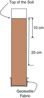

  

  Schematic of collected mesocosm with approximately 40 cm of soil within a 7.5 cm diameter, schedule 40 PVC pipe, 50 cm in length. A piece of geotextile fabric is taped to the bottom to prevent the soil from sliding out. Marks should be placed on the outside of the PVC at depths of 10 and 25 cm below the soil surface

  The depth from the top of the mesocosm to the top of the soil should be measured and then marked on the outside of the core. After this, mark the core at the 2 depths at which the Pt electrodes will be later installed. These depths will be at 10 and 25 cm below the top of the soil (NOT below the top of the PVC cylinder) as shown in Fig. 7.4.

• 3. Instrumentation of the mesocosms. An overview of the instrumentation is shown in Fig. 7.5 which illustrates how the mesocosm will appear when all the electrodes have been installed. Probably, the best order in which to install the electrodes is the following: (1) the deep (25 cm) Pt electrodes, (2) the salt bridge and calomel electrode; and (3) the shallow (10 cm) Pt electrodes.

  Fig. 7.5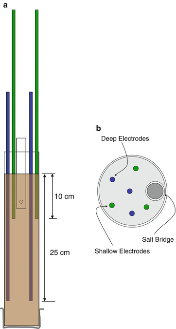

  

  Diagrams showing side view (a) and top view (b) of mesocosm indicating the spatial placement of the salt bridge and the Pt electrodes

• 4. Installing the deep electrodes. Note that the three deep Pt electrodes will be placed in an equally spaced arrangement around the mesocosm, optimizing the distance between the edge of the mesocosm and the future location of the salt bridge (see Fig. 7.5). Using colored tape, place a mark on each electrode that is 25 cm above the Pt point. Then, using a narrow sharpened stainless steel rod (slightly larger than the electrode), carefully make a VERTICAL pilot hole that is approximately ½ cm shallower than the depth where you will place the Pt electrode. Remove the rod and carefully slide a straight Pt electrode into the hole, and push the electrode to the exact depth where measurements are to be made (25 cm). Carefully install two additional deep electrodes in the same manner being sure to distribute them around the mesocosm (Fig. 7.5). Label these electrodes 25A, 25B, and 25C (for 25 cm below the soil surface).

• 5. Installing the salt bridge. The salt bridge is made from a piece of PVC pipe that has an OD of approximately 22 mm. It is filled with an agar which is saturated with KCl (similar to the calomel electrode itself) (Veneman and Pickering 1983). Prepare to use the salt bridge by inserting your previously selected (and tested) calomel reference electrode into the agar at the top of the salt bridge until the electrode is approximately 2–3 cm into the tube and the agar has encompassed the end of the electrode. Wipe any agar or salt from the electrode and PVC tube and carefully wrap with parafilm to produce a water tight seal that will hold the electrode in place. This will help to keep the electrode from drying out over time.

  A pilot hole approximately 5–10 cm deep should be made using a section of sharpened 2.5 cm dia. pipe, and the soil should be removed to make room for the salt bridge. Then insert the salt bridge firmly into the pilot hole, being careful that the agar does not slide out of the tube. The salt bridge should extend about 5–10 cm above the top of the soil.

• 6. Installing the shallow Pt electrodes. Mark each of the other three electrodes at a depth of 10 cm using colored tape. The three shallow Pt electrodes should be placed in an equally spaced arrangement around the mesocosm, much like the deep electrodes and following a similar installation procedure, but being careful not to disturb the other Pt electrodes or the salt bridge and calomel electrode (Fig. 7.5). Electrodes should be installed to a depth of 10 cm below the soil surface (which will be 15 cm above the deep electrodes) and should be labeled as electrodes 10A, 10B, and 10C.

• 7. Taking initial Eh measurements (prior to saturation). Using either a lab grade Eh meter or a multimeter in conjunction with a device to create a high resistance circuit (Rabenhorst et al. 2009; Rabenhorst 2009), the voltage should be measured in the circuit created between the calomel reference electrode and each Pt electrode. The positive (red) wire should attach to the Pt electrode and the black wire should connect to the reference electrode. When the electrodes have been recently installed, there may be some slight drift during the measurement, but this drift should become less apparent on subsequent days. Typically, these measurements are recorded to the nearest 0.001 V (note there is too much variability to warrant recording with any greater precision than this so make sure you are NOT reading to tenths of a mV). Commonly, students will occasionally reverse the wires on the volt meter when making measurements. This will result in VERY LARGE ERRORS, because the voltage will have the opposite sign (−300 mV vs. 300 mV). Be very careful to ensure that the Pt electrode leads to the red (+) pole on the volt meter and the reference electrode is connected to the black (−) pole. Your initial readings will probably be somewhere in the range of 200–400 mV (before correction for the reference electrode). Over time, the voltages will likely become lower (especially for the deep electrodes installed below the water table.) Note that pH measurements must also be obtained at the same 2 depths where the electrodes will be placed. It is recommended that soil pH at 10 and 25 cm be collected from a replicate mesocosm so that the instrumented mesocosm does not need to damaged.

• 8. Saturating the mesocosm. Mesocosms will be saturated to a depth of 15 cm below the soil surface. In order to saturate each mesocosm, stand the mesocosm vertically in a container (bucket) where the water can be adjusted to the proper height, and secure it using duct tape as shown in Fig. 7.6. Distilled water should then be added slowly to the bucket which will result in filling the soil pore space in the mesocosm from below, which should help minimize the entrapment of air during saturation. The water level should be raised until it is at the appropriate height (Fig. 7.7). An alternate arrangement is also shown in Fig. 7.7 where the mesocosm is saturated to the soil surface. This can be used to illustrate differences in properties of contrasting soil horizons (such as OM content in A vs. B horizons) if different soil materials occur at 10 vs. 25 cm.

  Fig. 7.6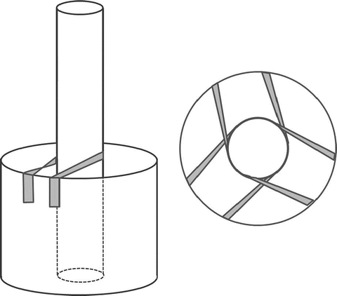

  

  Each mesocosm should be secured in a small bucket using three pieces of duct tape which wrap around the mesocosm and are affixed at approximately 120° from each other

  Fig. 7.7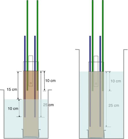

  

  On left, distilled water is added to the bucket until it reaches a level 15 cm below the soil surface. The tips of shallow and deep Pt electrodes should be located 5 cm above the water level and 10 cm below the water level, respectively. Water should be added periodically to preserve the desired level. An alternate arrangement (shown on right) is to use a taller bucket and to saturate the mesocosm to the soil surface. This can be especially informative if soil horizons with contrasting properties (such as OM content) occur at depths of 10 and 25 cm

• 9. Eh measurements after saturation. Approximately 30–60 min after saturation, collect the second set of Eh measurements from the mesocosm as described previously. After this, Eh measurements should be made on the mesocosms daily for the first week, and then every other day through subsequent weeks. This should be continued for a minimum of 2 weeks and may produce better results if extended for 3 or 4 weeks. The level of the water in the bucket will need to be checked and maintained at the proper height.

• 10. Disassembly of the mesocosms. At the end of 2 (or more) weeks, remove the mesocosm from the water reservoir and place it on some absorbent material (newspaper) and allow it drain. Empty the water from the bucket into appropriate containers in the lab (do not empty soil down the sinks!)

  Carefully remove each of the Pt electrodes trying not to disturb the soil too much. Rinse off the Pt electrodes and set aside in a group being careful to keep them together and labeled with your mesocosm number. Check each electrode by placing them in the Light’s solution and determining the voltage measured using a common calomel reference. This should be done to determine if any appear to be malfunctioning (in which case, data from those electrodes should not be included in the analysis).

  Remove the calomel reference electrode from the salt bridge, rinse off the electrode and make sure it is adequately filled with saturated KCl before storing. Using a rod, pole, or other device, extrude the soil from the PVC sleeve onto newspaper, trying to keep the core as intact as possible.

• 11. Testing for Ferrous Fe using alpha-alpha dipyridyl (ααd) dye (or strips).³ Using a knife or spatula, split open the extruded core lengthwise, trying mainly to break open and expose the fresh soil surface (rather than a knife-cut soil surface). Note that you will need to test the freshly exposed and broken soil surface with the ααd (sometimes a false positive reaction to ααd is detected from where the low valence Fe from the steel in a knife blade or shovel has contacted the soil.)

  Place a few drops of ααd (Childs 1981) on one-half of the core at various depths along the length of the mesocosm and note whether there is a reaction. Look for a pink color to develop. (If there is a lot of Fe²⁺ in the soil solution, this can sometimes occur quite rapidly. Other times, if there is very little Fe²⁺ in solution, it may take a few minutes for a subtle reaction to be observed.) In particular, pay attention to whether there is a reaction in the vicinity of where you had placed the electrodes (10 and 25 cm below the soil surface). Also keep in mind, the depth at which the water table was maintained in your mesocosm.

  Record your observations (especially at the depths of the electrodes), noting whether the reaction to ααd was negative, or positive, and if positive, indicate whether you think the reaction was weak, moderate or strong. Document any reaction to ααd at various other places up and down the core to try to obtain a better sense of where in the soil, Fe³⁺ has been reduced to Fe²⁺. If you observe a positive reaction to ααd in the soil core, be careful to document where in the soil that reaction was observed, especially in relation to where the water table was located within the soil.

• 12. Measuring soil pH. In order to be able to plot data on an Eh-pH diagram, you will need to measure the pH of the soil at the same depths where you measured Eh. Use the OTHER HALF of the core to which you did NOT apply the ααd for measuring pH. Collect a few (10) ml of soil material from each of the two depths where Eh was measured and make a thick slurry by adding distilled water and stirring (the goal is the equivalent of 1:1 soil:water, but as you are not starting with dry soil, this will be an approximation). Allow the slurry to sit for 10–15 min and then mix again. Measure the pH by using a calibrated pH meter with a combination electrode and record to the nearest 0.1 units.

• 13. Data Analysis. Eh data should be reported in three ways. First, these data should be plotted as a function of time. This will allow you do evaluate whether any of the readings from any of the electrodes was spurious. Normally, a given electrode will show trends over time, and not provide erratic readings. If all the readings for a given electrode follow a trend and then one reading is way off, there is a good chance that the one reading is faulty. An example of Eh data plotted in this way is shown in Fig. 7.8.

  Fig. 7.8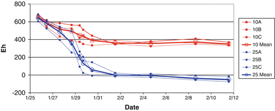

  

  Plotting of Eh measurements as a function of time. Note that replicate Eh measurements sometimes vary by more than 100 mV

  The second way in which the mesocosm data should be evaluated is with regard to an Eh-pH stability diagram. This is to determine whether the soil conditions were (theoretically) reducing with respect to Fe at any time during the experiment. You will only have pH measurements from your mesocosm at beginning and end of the experiment, and the pH is not be expected to change dramatically over the course of a couple of weeks (often one unit or less). For the sake of simplification, we will make the assumption that the pH changed gradually (linearly) through the period of the experiment and thus use interpolated data for the dates in between. When plotted, these data may look something like those in Fig. 7.9. Also shown in Fig. 7.9 is the line for the equation Eh = 595 − (60 pH). This is the equation from the technical standard of the NTCHS (sometimes referred to as the “Technical Standard” line) (National Technical Committee for Hydric Soils 2007). This is an empirically derived line (shown in green), and data that plot above this line are considered to be oxidizing and those below the line indicate reducing conditions. The Eh-pH line showing the stability field for the crystalline iron oxide mineral goethite is also shown on the diagram (brown). Some people prefer to discuss iron reduction and Eh-pH data with respect to predictions using thermodynamically based equations such as this one. Above the line, goethite would be predicted to be stable and below the line, it would be predicted to unstable with Fe³⁺being reduced to Fe²⁺.

  Fig. 7.9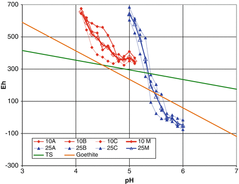

  

  Example data from mesocosms plotted on an Eh-pH diagram. Also shown is the “technical standard” line (TS) from the National Technical Committee for Hydric Soils which they use to define reducing soil conditions and also the stability line for goethite-Fe²⁺

  A third, and perhaps even more useful way to view the data is to plot the data over time, with the Eh values relative to the TS line (or this could also be done with respect to the a line like the goethite line). This is done by using pH data (for each date and depth) to calculate the corresponding Eh along the TS line, using the equation Eh = 595 − (60 pH). For example, if the pH ranged from 4.1 to 5.1 over a 6 day period, we would calculate the corresponding Eh values as shown in Table 7.5 (these change from 349 to 289 as the pH changes from 4.1 to 5.1).

  Table 7.5 Calculation of Eh data with respect to the Technical Standard Line of the NTCHS

  These calculated values can then be subtracted from the measured Eh values (made using Pt electrodes). Positive values indicate that they are above the TS line (oxidizing) and if the values are negative, this means the data would plot below the TS line (reducing). If the data shown in Fig. 7.8 are plotted relative to the TS line, we obtain the graph shown in Fig. 7.9. On the graph in Fig. 7.9, the “zero” of the Y axis (Eh relative to the TS) represents the TS line itself. So any values that are greater than zero imply that the data plot above the TS line (in an Eh pH diagram) and are oxidizing with respect to Fe, and any negative values imply that the data plot below the TS line and are reducing with respect to Fe. This plot allows a quick visual evaluation of how these conditions change with time and at what point in time they become reducing.

7.1.2.2.5 Submission of Lab Report

Each student will write and submit a laboratory report based upon the data collected by the group (in the table below, data collected by students are shown by the shaded boxes). Each student should then calculate the Eh (considering the correction for the reference electrode). A graph similar to Fig. 7.8 should be constructed. The Eh of the TS line should be calculated for the pH values measured (and interpolated) for the soil. Then you should calculate, for each electrode, the Eh relative to the TS.

Using data measured and calculated in the student’s version of Table 7.6, each of the following figures should be prepared:

Table 7.6 Draft data sheet for recording measurements and calculations to be used in later analyses and figures

• A figure showing Eh over time (similar to Fig. 7.8)

• A figure showing Eh and pH in relation to the TS line and to the goethite stability line (similar to Fig. 7.9)

• A figure showing Eh relative to the TS as a function of time (similar to Fig. 7.10)

  Fig. 7.10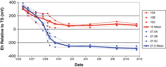

  

  Plot showing how Eh values are related to the Technical Standard line of the NTCHS, as a function of time. Positive values (above zero) indicate that the Eh is above the TS line (and thus is oxidizing). When values drop below zero, it indicates reducing soil conditions

Each student should provide a discussion of the data and figures that should include some reference to the following:

• Reproducibility and replication of the data measurements;

• Comparison of redox data collected at the two soil depths;

• The meaning of the Eh/pH data collected, implications of the data based on Eh/pH stability diagrams and where data plot relative to the TS line; and

• Comparisons between methods used – in particular the Eh/pH data and the reaction of the soil with alpha-alpha dipyridyl dye.

7.1.2.2.6 References

Childs CW (1981) Field test for ferrous iron and ferric-organic complexes (on exchange sites on in water-soluble forms) in soils. Aust J Soil Res 19:175–180

Light TS (1972) Standard solution for redox potential measurements. Anal Chem 44:1038–1039

National Technical Committee for Hydric Soils (2007) Technical note 11: technical standards for hydric soils. USDA-NRCS, Washington, DC. ftp://ftp-fc.sc.egov.usda.gov/NSSC/Hydric_Soils/note11.pdf

Owens PR, Wilding LP, Lee LM, Herbert BE (2005) Evaluation of platinum electrodes and three electrode potential standards to determine electrode quality. Soil Sci Soc Am J 69:1541–1550

Rabenhorst MC (2009) Making soil oxidation-reduction potential measurements using multimeters. Soil Sci Soc Am J 73:2198–2201

Rabenhorst MC, Hively WD, James BR (2009) Measurements of soil redox potential. Soil Sci Soc Am J 73:668–674

Veneman PLM, Pickering EW (1983) Salt bridge for field redox potential measurements. Commun Soil Sci Plant 14:669–677

7.1.3 Field Exercises

7.1.3.1 Field Exercise 1: Use and Interpretation of IRIS Tubes

7.1.3.1.1 Objectives

• 1. To understand the principles behind the use of IRIS tubes.

• 2. To understand how to use IRIS tubes in the field.

• 3. To understand how to interpret the data from IRIS tubes.

• 4. To compare the functioning of IRIS tubes with other measures of reduction in soils.

7.1.3.2 Part I: IRIS Tube Installation

7.1.3.2.1 Materials and Equipment Needed

• Five IRIS tubes

• 7/8″ push probe for making pilot holes

• Spade or shovel

• Tape measure

• Transparent mylar grids

• Equipment for making Eh measurements

• Five, 40 cm Pt wire electrodes

• One reference electrode (with salt bridge)

• One, high impedance voltmeter

• pH meter and buffers (This can be done in the field using a portable meter, or else samples can be returned to the lab for pH measurement.)

• Alpha, alpha dipyridyl dye solution or test strips

7.1.3.2.2 Procedures

Overview: IRIS tubes will be installed following protocols spelled out in the Rabenhorst (2008) article. Tubes will remain in the soil for 4 weeks, after which they will be examined and paint removal will be quantified. On the dates on which the tubes are installed and extracted, water table levels will be documented. Also on these dates, soil reduction will be assessed using Eh (and pH) measurements and also by testing with alpha, alpha dipyridyl dye. Comparisons will be made among all three methods for assessing soil reduction.

• 1. Students should work in teams of 3–4 persons.

• 2. Each team will install a set of five IRIS tubes in the field (at a site provided by the instructor), following protocols spelled out in the Rabenhorst (2008) article.

• 3. At the location where the IRIS tubes were installed, an estimation of the level of the ground water table should be obtained by digging a small hole to a depth slightly greater than the depth to the water table and allowing it to equilibrate in the hole.

• 4. At the location where the IRIS tubes were installed, Eh should be measured using five replicate Pt electrodes at depths of 12.5, 25, and 40 cm. A stainless rod should be used to make pilot holes for the electrodes to the specified depths. First the five electrodes should be placed at 12.5 cm and measurements made. Then the pilot holes should be deepened and electrodes placed at 25 cm and measurements made a second time. A third set of measurements should be made after electrodes have been placed at 40 cm. Because electrodes will not remain in the field between the two measurement dates, the reference electrode does not need to be placed within a salt bridge. Rather, a small amount of water should be added to the soil surface (if not already saturated) and stirred to make a paste, into which the reference electrode should be placed. The reference electrode should be situated within 25–75 cm of the location of the Pt electrodes.

• 5. Using either the push probe, a spade or an auger, samples should be collected from depths of 12.5, 25 and 40 cm so that pH can be determined at the same depths where Eh was measured.

• 6. Using either soil on cores removed when making pilot holes for IRIS tubes or soil collected with a spade or auger, apply a few drops of alpha-alpha dipyridyl dye at various depths in the soil to see whether there is a positive reaction to the dye, indicating the presence of Fe²⁺.

• 7. Make a brief soil description at the location where the IRIS tubes were installed making special note regarding whether or not the soil meets any of the approved field indicators of hydric soils (USDA-Natural Resources Conservation 2010).

• 8. After approximately 4 weeks have elapsed, on the date when the IRIS tubes are extracted and examined, you should again make measurements of Eh, pH and water table height, and evaluate whether the soil gives a positive reaction to the alpha-alpha dipyridyl dye.

7.1.3.3 Part 2: IRIS Data Collection and Analysis

• 1. Four weeks after the IRIS tubes were installed, they should be extracted from the soil. Adhering soil can be removed by rinsing with very gentle brushing (as needed) under a stream of water, and then placed aside to dry.

• 2. Quantification will be accomplished using the mylar grid method (Rabenhorst 2012)because this method is more accurate and more reproducible than visual estimations (Rabenhorst 2010). A 15 cm by 6.7 cm grid containing 390 50 mm by 51 mm sectors should be printed on transparent mylar sheet so that it can be wrapped around an IRIS tube and held in place using rubber bands (Fig. 7.11).

  Fig. 7.11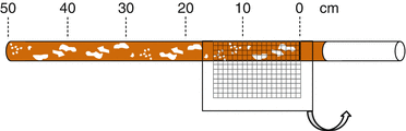

  

  Illustration showing placement of mylar grid around a 15 cm portion of an IRIS tube. By marking and counting sectors where paint has been removed, paint removal can be easily quantified (Modified from Rabenhorst 2012 with kind permission of © The Soil Science Society of America, Inc. 2012. All Rights Reserved)

• 3. The Technical Standard (National Technical Committee for Hydric Soils 2007) requires that paint be removed from 30 % of the IRIS tube within a 15 cm zone that occurs somewhere within the upper 30 cm of the soil.⁴ Therefore each group must determine which 15 cm zone within the upper 30 cm of each IRIS tube shows the maximum paint removal, and quantification should proceed for this zone.

• 4. A clear mylar grid should be wrapped around that portion of each IRIS tube showing the greatest degree of paint removal and should be secured using rubber bands. Using a fine point permanent marker, each sector with greater than 50 % paint removal should be marked. Once all the sectors are marked, the sectors should be counted and the percentage of the area can be calculated.

7.1.3.4 Part 3: Comparison of IRIS Data with Eh, pH and ααd Data

• 1. Using Eh and pH data collected and plotted on an Eh-pH stability diagram you should be able to evaluate whether the soil is reducing (or at what depths, the soil is reducing).

• 2. Based on the data you have collected, you now have 3 independent assessments of whether the soil is reducing: (1) Eh-pH; (2) ααd; (3) IRIS tubes.

• 3. Provide a thorough discussion of your data, being sure to include:

  • A summary of whether or not the soil was reducing according to each of the three assessment tools;

  • How results from each of these assessment methods were similar to or different from the others;

  • What factors might account for any differences that you observed; and

  • Your own conclusions (based upon your data) regarding whether or not the soil is reducing. Note that according to the Technical Standard of the NTCHS, in order for a soil to be reducing, it must meet the reducing specifications of one of the three methods, within the zone of 0–30 cm for a period of 14 days. For Eh and IRIS, a majority of the instruments (three-fifth) must fall within the specified range (not the mean).

• 4. Your submitted lab report should include the following:

  • Data tables showing all data collected on each of the two dates (Eh, pH, ααd, temperature, water tables);

  • Your discussion of water tables and temperatures over the course of the month (using your data and the continuous class record);

  • Completed IRIS data forms with data from yourself and from others in your group;

  • Eh-pH diagrams showing your data plotted for each of the two dates;

  • Your soil description and assessment regarding whether the soil meets any of the Field Indicators; and

  • Your complete discussion of all the data (including morphological data) with your conclusions.

7.1.3.4.1 References

National Technical Committee for Hydric Soils (2007) Technical note 11: technical standards for hydric soils. USDA-NRCS, Washington DC. Available from: ftp://ftp-fc.sc.egov.usda.gov/NSSC/Hydric_Soils/note11.pdf

Rabenhorst MC (2008) Protocol for using and interpreting IRIS tubes. Soil Surv Horiz 49:74–77

Rabenhorst MC (2010) Visual assessment of IRIS tubes in field testing for soil reduction. Wetlands 30:847–852

Rabenhorst, MC (2012) Simple and reliable approach for quantifying IRIS tube data. Soil Sci Soc Am J 76:307–308

USDA, NRCS (2010) Field indicators of hydric soils in the United States. Ver. 7.0. In: Vasilas LM, Hurt GW, Noble CV (eds) USDA, NRCS in cooperation with the National Technical Committee for Hydric Soils

7.1.3.5 Field Exercise 2: Assessing Leaf Litter Decomposition with Litter Bags

7.1.3.5.1 Objectives

• 1. To understand the principles behind the use of litter bags.

• 2. To understand how to construct and deploy litter bags.

• 3. To understand the impact of soil moisture content on decomposition rates.

7.1.3.5.2 Materials and Equipment Needed

• Leaf litter samples

• Litter bags – fiberglass screening material, mesh size of 1–2 mm

• Drying oven

• Balance

• Pin flags

7.1.3.5.3 Procedures

Overview: There are several options with this exercise with respect to the type of organic materials used and the location of bag deployment in the field. In the procedures below, we suggest collecting fallen leaves from one deciduous tree species. This is the simplest approach and promotes uniformity in the samples. However, the exercise can be modified to compare multiple species or even root samples. With respect to deployment location, we suggest two sites, a wetland and an adjacent upland. The main point to this exercise is that wet conditions slow down decomposition rates. To further illustrate this point, the class may choose to place some litter bags in inundated areas. We suggest avoiding permanently inundated areas as it may be difficult to retrieve the bags.

• 9. Litter bag construction. Ten litter bags will be needed for each team of students. For each litter bag cut a 20 cm × 40 cm section of screen. Double the screen section over and staple the sides together at 5 cm intervals. You should now have a screen pouch open at one end. The open end will be stapled shut after the bag is filled with leaf litter. Each bag should be numbered with a permanent marker for future identification. Weigh each bag with three additional staples. Record the weight. The weight of the additional staples is needed to account for the staples used to close the open end of the bag after the leaf sample is added.

• 10. Leaf litter sample collection. Collect fallen leaves from the chosen field site. To promote uniformity in the samples; collect all samples from the adjacent upland, sample only the top layers of the litter, and sample only one deciduous tree species.

• 11. Sample preparation. Chop the leaves into 2–5 cm lengths. Randomly collect five sub-samples of the chopped leaves. Determine fresh weight of the sub-samples, then dry them (70 °C, 48–72 h) and re-weigh to obtain their water content.

• 12. Bag filling. Fill the bags with the prepared samples. Try to place a similar amount of material in each bag (It does not need to be exactly the same). The material should be relatively loose in the bag to allow for air movement. Staple the open end closed with three staples. Weigh each bag and record. Sample fresh weight is calculated as the difference between the filled bag weight and the empty bag weight.

• 13. Litter bag deployment. Place five bags in the upland and five bags in the wetland. For placement in the wetland, choose deployment points with similar hydrologic conditions as soil moisture will impact decomposition rates. For example, if the site has pit and mound topography, do not place 1 bag on top of a mound and another bag in a pit. Avoid permanently inundated areas. Clear away any duff and place the bags directly on top of the mineral soil surface. Mark the location of each bag with a pin flag.

• 14. Litter bag retrieval and analysis. Retrieve the bags after 2–3 months. Dry the retrieved bags (70 °C, 48–72 h) and weigh. Calculate sample dry weight.

• 15. Calculations. Loss of biomass due to decomposition is calculated as the difference between initial biomass and remaining biomass. All values are expressed on a dry weight basis. Initial dry weight (pre-deployment) of the samples is calculated from the fresh weight of each sample and the average water content of the five sub-samples determined in Step 3. Average rate of decomposition (per day) is determined by dividing biomass loss by the incubation period. Compare the mean biomass loss for the upland samples to that of the wetland samples.

References

Aber JP, Melillo JM (1980) Litter decomposition: measuring state of decay and percent transfer in forest soils. Can J Bot 58:416–421
Aitkenhead-Peterson JA, McDowell WH, Neff JC (2003) Sources, production, and regulation of allochthonous dissolved organic matter inputs to surface waters. In: Findlay S, Sinsabaugh R (eds) Aquatic ecosystems: interactivity of dissolved organic matter. Academic Press, Amsterdam, pp 26–70
Altor AE, Mitsch WJ (2008) Pulsing hydrology, methane emissions and carbon dioxide fluxes in created marshes: a 2-year ecosystem study. Wetlands 28:423–438
Avery EA, Burkhart HE (2002) Forest measurements, 5th edn. McGraw-Hill Higher Education, New York
Barackman M, Brusseau ML (2004) Groundwater sampling. In: Artiola JF, Pepper IL, Brusseau ML (eds) Environmental monitoring and characterization. Elsevier Academic Press, Burlington, pp 121–141
Barth DS, Mason BJ (1984) The importance of an exploratory study to soil sampling quality assurance. In: Schweitzer GE, Santolucito JA (eds) Environmental sampling for hazardous wastes. American Chemical Society, Washington, DC, pp 97–104
Barth DS, Mason BJ, Starks TH, Brown KW (1989) Soil sampling quality assurance user’s guide, 2nd edn. Environmental Monitoring and Support Laboratory. USEPA Report No. EPA/600/8-89/046, Las Vegas
Benner R (2003) Molecular indicators of the bioavailability of dissolved organic matter. In: Findlay SEG, Sinsabaugh RL (eds) Aquatic ecosystems: interactivity of dissolved organic matter. Academic Press/Elsevier Science, San Diego, pp 121–137
Bernier P, Hanson PJ, Curtis PS (2008) In: Hoover CM (ed) Field measurements for forest carbon monitoring. Humana Press, New York, pp 91–101
Blake GR, Hartge KH (1986) Bulk density. In: Klute A (ed) Methods of soil analysis, Part 1. Physical and mineralogical methods, SSSA Book Series No. 5. Soil Science Society of America, Madison, pp 363–376
Bloomfield J, Vogt K, Wargo PM (1996) Tree root turnover and senescence. In: Waisel Y, Eshel A, Kafkafi A (eds) Plant roots: the hidden half, 2nd edn. Marcel Dekker, New York, pp 363–381
Boddey RM (1987) Methods for quantification of nitrogen fixation associated with Gramineae. CRC Crit Rev Plant Sci 6:209–266
Bohlen PJ, Gathumbi SM (2007) Nitrogen cycling in seasonal wetlands in subtropical cattle pastures. Soil Sci Soc Am J 71:1058–1065
Bohn HL (1971) Redox potentials. Soil Sci 112:39–45
Bradford JB, Ryan MG (2008) Quantifying soil respiration at landscape scales. In: Hoover CM (ed) Field measurements for forest carbon monitoring. Humana Press, New York, pp 143–162
Bremner JM (1996) Nitrogen-total. In: Sparks DL (ed) Methods of soil analysis, Part 3. Chemical methods, SSSA Book Series No. 5. Soil Science Society of America, Madison, pp 1085–1122
Bridgham SD, Updegraff K, Pastor J (1998) Carbon, nitrogen, and phosphorous mineralization in northern wetlands. Ecology 79:545–561
Brown JR (ed) (1987) Soil testing: sampling, correlation, calibration, and interpretation, SSSA Spec Publ No 21. Soil Science Society of American, Madison, p 144
Bruland GL, Richardson CJ, Daniels WL (2009) Microbial and geochemical responses to organic matter amendments in a created wetland. Wetlands 29:1153–1165
Butterly CR, Bunemann EK, McNeill AM, Baldock JA, Marschner P (2009) Carbon pulses but not phosphorus pulses are related to decreases in microbial biomass during repeated drying and rewetting of soils. Soil Biol Biochem 41:1406–1416
Cahoon DR, Turner RE (1989) Accretion and canal impacts in a rapidly subsiding wetland: II. Feldspar marker horizon technique. Estuaries 12:260–268
Cahoon DR, Lynch JC, Hensel PF, Boumans RM, Perez BC, Segura B, Day JW Jr (2002a) High precision measurement of wetland sediment elevation: I. Recent improvements to the sedimentation-erosion table. J Sediment Res 72:730–733
Cahoon DR, Lynch JC, Perez BC, Segura B, Holland R, Stelly C, Stephenson G, Hensel PF (2002b) High precision measurement of wetland sediment elevation: II. The rod surface elevation table. J Sediment Res 72:734–739
Callaway JC, Desmond JS, Sullivan G, Williams GD, Zedler JB (2001) Assessing the progress of restored wetlands: hydrology, soil, plants, and animals. In: Zedler JB (ed) Handbook for restoring tidal wetlands. CRC Press, Boca Raton, pp 271–335
Carpenter EJ, van Raalte CD, Valiela I (1978) Nitrogen fixation by algae in a Massachusetts salt marsh. Limnol Ocean 23:318–327
Castenson KL, Rabenhorst MC (2006) Indicator of reduction in soil (IRIS): evaluation of a new approach for assessing reduced conditions in soil. Soil Sci Soc Am J 70:1222–1226
Champagne P (2008) Wetlands. In: Ong SK, Surampalli RY, Bhandari A, Champagne P, Tyagi RD, Lo I (eds) Natural processes and systems for hazardous waste treatment. American Society of Civil Engineers, Reston VA, pp 189–256