Assessing and Measuring Wetland Hydrology

Abstract

Virtually all ecological processes that occur in wetlands are influenced by the water that flows to, from, and within these wetlands. This chapter provides the “how-to” information for quantifying the various source and loss terms associated with wetland hydrology. The chapter is organized from a water-budget perspective, with sections associated with each of the water-budget components that are common in most wetland settings. Methods for quantifying the water contained within the wetland are presented first, followed by discussion of each separate component. Measurement accuracy and sources of error are discussed for each of the methods presented, and a separate section discusses the cumulative error associated with determining a water budget for a wetland. Exercises and field activities will provide hands-on experience that will facilitate greater understanding of these processes.

Student Exercises

3.1.1 Classroom Exercises

3.1.1.1 Short Exercise 1: Converting Pressure to Water Depth and Stage

Measuring wetland stage and hydraulic head, and determining direction and potential for flow between groundwater and surface water, are among the most basic requirements in wetland hydrology. A sketch of a common monitoring installation appears below (Fig. 3.34). A piezometer designed to indicate hydraulic head beneath the wetland bed is instrumented with a submersible pressure transducer. The sensor is suspended from the surface of the well casing by a metal wire. The distance from the attachment point to the sensor port commonly is described as the hung depth. This particular type of sensor stores the data on a circuit card; the sensor must be retrieved and the data downloaded periodically. Some installations instead have a data cable extending from the sensor to a datalogger that can query and store data from multiple sensors. In some models the cable contains a vent tube that allows changes in atmospheric pressure to be transmitted to the pressure sensor. Venting allows the pressure measurement to be relative to atmospheric pressure. The transducer in this example is not vented to the atmosphere; some would argue this is preferable because there is no associated opportunity for water vapor to reach and damage the sensor electronics. However, without venting, the sensor output is the sum of hydrostatic pressure of the water column above the sensor port (the dwc or depth of the water column that we want to know) and atmospheric pressure. Therefore, atmospheric pressure needs to be measured and subtracted from the output of the submerged pressure transducer to obtain the height of the water column above the submerged sensor. A barometer is suspended in the piezometer casing, well above the water level, to provide atmospheric-pressure measurements. If the well is susceptible to occasional flooding, the barometer could instead be located anywhere nearby as atmospheric pressure does not change appreciably over distances of several km.

Fig. 3.34

Installations commonly used to determine wetland stage, elevation, and vertical hydraulic-head gradient

Output from pressure transducers, as well as many other sensors, commonly is converted to units in which field check measurements are made. In wetland settings, that unit usually is feet or meters of water head. Meters will be used here. To convert output in pressure to head, recall that Pressure = ρgh where ρ is density of water (kg m⁻³), g is acceleration due to gravity (m s⁻²), and h, hydraulic head, is the height to of a column of liquid that would exert a given pressure, in m. Output from pressure transducers commonly is in units of Pascals. Recall that a Pascal is a Newton per square meter and that a Newton, a unit of force, is determined in terms of mass times acceleration (kg m s⁻²). Therefore,

$$ h=\frac{{{P_{trans }}-{P_{bar }}}}{{\rho g}}+Offset $$

(3.55)

where P _trans is the output from the submerged pressure transducer, P _bar is the output from the barometer, and Offset is a value that equates the sensor output to a local datum or reference elevation.

A stilling well also is displayed in the drawing. Although another submerged pressure transducer could have been used to indicate wetland stage, this stilling well contains a float and counterweight that together rotate a pulley connected to a potentiometer or pulse-counting device. As water level changes, the float moves and the pulley rotates, changing either the electrical resistance if the sensor is a potentiometer, or causing electrical pulses to be sent to a data recording unit if the sensor is a pulse-counting device (often called a shaft encoder). The output of the sensor in the stilling well commonly is set to be equal to the water level indicated by a nearby staff gage.

The staff gage is connected to a metal pipe driven into the wetland bed. This simple device is designed to provide a direct indication of the relative stage of the wetland. The units on the “staff plate” in this example are in meters, but units of feet are perhaps more common in the US. Some wetland sediments are relatively soft, and some wetlands freeze during winter, providing the potential for the staff gage to move over time. To determine whether this occurs or not, we need a stable reference point to which the staff gage can be compared; hence, the reference mark, commonly called an RM. The term RM is used so as to not confuse it with BM (bench mark), which is an official surveying location that is part of a national geodetic survey. This particular RM consists of a pipe that extends into the ground. However, in areas where soil frost is common and can extend a meter or more beneath ground surface, pipes also can move. Therefore, this particular RM was set in a mass of concrete that was installed beneath the deepest expected extent of soil frost.

Our tasks here are to:

• 1. compare the potentiometer output from the stilling well to the output from the submerged pressure transducer in common units,

• 2. make separate measurements of water levels inside of the well and of the wetland surface,

• 3. determine the difference in hydraulic head (Δh) between the wetland and the piezometer, and

• 4. verify that our sensors are providing the correct output.

Field site data
Staff gage	0.750 m (manually read)
Potentiometer	0.755 m
dts	0.198 m (manually measured)
dtw	0.178 m (manually measured)
Barometer	100.510 kPa
Pressure transducer	110.610 kPa
Pressure-transducer offset	−0.250 m

• 1. What is the dwc in m of water? Assume fresh water at 20 °C. (therefore, density = 998 kg/m³)________________________________

• 2. What does the pressure transducer indicate for head in the piezometer in m relative to the local datum?________________________________

• 3. What do the sensors indicate for Δh?____________________________

• 4. What is the manually measured Δh?____________________________

• 5. Is the potential for flow upward or downward based on the measured values?____________________________

• 6. How does the Δh indicated by the sensors differ from the Δh calculated from the manual measurements?____________________________

• 7. What is the gradient assuming the midpoint of the well screen is 0.75 m below the wetland bottom?____________________________

• 8. If the top of the staff gage plate is at an elevation of 102.550 m, what is the elevation of the water level inside of the piezometer?____________________________

3.1.1.2 Short Exercise 2: Wind Correction of Precipitation Data

Table 3.3 shows daily mean air temperature and wind speed, and daily total precipitation recorded by a weighing precipitation gauge with an Alter wind shield (similar to Fig. 3.5a), at a hydrological research station in Calgary, Alberta, Canada, in 2008. There were two precipitation events, on December 7 and 12.

Table 3.3 Daily mean air temperature and wind speed, and daily total precipitation

• 1. Based on the air temperature, determine the form of precipitation (rain or snow).

• 2. If the precipitation occurs as snow, then a correction must be made to account for the gage-catch deficiency (see Fig. 3.6). Use the following equation (Dingman 2002:111–112) to compute the catch deficiency factor (CD) from wind speed (u, m s⁻¹) for each day.

  $$ \mathrm{ CD}=100 \exp \left( {-4.61-0.036{u^{1.75 }}} \right) $$

  (3.56)

• 3. Divide the uncorrected precipitation by CD to estimated true (i.e., corrected) precipitation.

• 4. Calculate the total of two precipitation events for both uncorrected and corrected data. What is the degree (percentage) of underestimate by not correcting the data?

• 5. Many winter precipitation data sets available on the internet have not been corrected. Discuss the potential problem of using such data for a water-budget analysis.

3.1.1.3 Short Exercise 3: Spatial Interpolation of Precipitation Data

Table 3.4 shows monthly total precipitation (mm) at three meteorological stations in Alberta, Canada. Olds Station is located between two other stations, approximately 50 km south of Red Deer and 70 km north of Calgary. The first three columns list the long term average for 1971–2000; the last three columns list the data recorded in 2010. The 2010 data for Olds are missing.

Table 3.4 Long-term average monthly precipitation and 2010 monthly precipitation (mm) at three meteorological stations in Alberta, Canada

• 1. Using the normal ratio method (Eq. 3.7), estimate monthly total precipitation in Olds for the three missing months.

• 2. Actual precipitation data recorded at the Olds station were 77 mm for June, 85 mm for July, and 79 mm for August. Discuss the magnitude of uncertainty associated with this method.

3.1.1.4 Short Exercise 4: Calculation of Discharge from Tracer Data

Tracer dilution methods were used to estimate the discharge of two small streams flowing into a wetland. The constant injection method was used in the first stream, where chloride solution having a concentration of 60 g L⁻¹ was injected at a rate of 12 L min⁻¹. The tracer concentration in the stream reached a steady value of 100 mg L⁻¹ by 150 s after the start of injection (Fig. 3.35). The background chloride concentration in the stream was 1 mg L⁻¹.

Fig. 3.35

Concentration of chloride tracer in streams. Left: constant-rate injection test. Right: slug injection test

• 1. Using Eq. 3.23, estimate the stream discharge from concentration data.

  The slug injection method was used in the second stream, where 10 L of tracer solution containing 3 kg of chloride mass was instantaneously injected in the stream. The tracer concentration reached a peak about 40 s after the release and declined quickly afterwards (Fig. 3.35). The background chloride concentration in the stream was 2 mg L⁻¹. Concentration data are listed in Table 3.5.

  Table 3.5 Data for slug injection test

• 2. Using Eq. 3.25 with Δt = 10 s, estimate the integral in the denominator of Eq. 3.24.

• 3. Using Eq. 3.24 with C ₁ V ₁ = 3 kg, estimate the stream discharge.

3.1.1.5 Short Exercise 5: Calibration of Weir Coefficient

V-notch weirs provide stable and reliable flow measurements, particularly when the coefficient C in the weir formula (Eq. 3.28) is determined to reflect site-specific conditions. Table 3.6 lists measurements of water level (h) and discharge (Q) for the V-notch weir shown in Fig. 3.11b. The water level is measured with respect to the base of the weir. Therefore, h ₀ = 0 in Eq. 3.28.

Table 3.6 Water level (h) in a 90° V-notch weir and independently measured discharge (Q) in the weir shown in Fig. 3.11

• 1. Compute h ^5/2 and convert Q to m³ s⁻¹.

• 2. Plot h ^5/2 and Q in the graph and determine the slope of the plot.

• 3. Determine C in Eq. 3.28. Note that θ = 90°; thus, tan(θ/2) = 1. Compare this value to the theoretical value for an ideal weir, C = 1.38.

3.1.1.6 Short Exercise 6: Determination of Stage-Discharge Rating Curve

Coefficients for the stage-discharge rating curve (Eq. 3.26) of a stream gauging station can be determined from a series of measurements of stage (h) and discharge (Q) encompassing different flow conditions. Table 3.7 lists the measured h and Q in a small stream in Calgary, Alberta, Canada. The stage at zero flow (h ₀) is 0.35 m at this gauging station. Equation 3.28 can be written in a logarithmic form

$$ \log Q = \log a+m \log \left( {h - {h_0}} \right) $$

(3.57)

When the logarithms of data are used to fit a straight line, the intercept and slope of the line give loga and m, respectively.

Table 3.7 Water stage (h) and discharge (Q) measured in a small stream near Calgary, Alberta, Canada in 2011

• 1. Compute log(h − h ₀) and logQ for each measurement.

• 2. Plot log(h − h ₀) and logQ in the graph and fit a straight line.

• 3. Determine the intercept and the slope of the plot, and compute a and m.

3.1.1.7 Short Exercise 7: Estimation of Diffuse Overland Flow

The amount of diffuse overland flow can be estimated using a wetland as a natural overland flow trap. If the wetland does not have inflow or outflow streams, and the contribution of groundwater flow is negligible during a short-duration storm, then the water balance equation for the wetland pond is given by Eq. 3.32. Total overland flow during the storm (O _ftot ) is estimated from measuring the volume of pond water before (V _ini ) and after (V _fin ) the storm. The figure embedded in Table 3.8 shows the pond stage and cumulative precipitation in Wetland 109 in the St. Denis National Wildlife Area in Saskatchewan, Canada, on July 4–5, 1996 (see Hayashi et al. 1998 for a site description). The cumulative precipitation (p _cum ) during the entire storm was 51 mm. The pond stages recorded at 21:00 and 02:00 are listed in Table 3.8. Water depth (H) at the deepest point in the pond is given by subtracting 551.68 m from the pond stage. The area of pond surface (A) and the volume of pond water (V) can be estimated using Eqs. 3.4 and 3.5 with s = 3,180 m² and p = 1.61 (Hayashi and van der Kamp 2000). The effective drainage area (A _eff ) of Wetland 109 is 20,100 m².

Table 3.8 Pond stage in Wetland 109 in the St. Denis National Wildlife Area, Saskatchewan, Canada on July 4, 1996

• 1. Calculate the initial (21:00) and final (02:00) pond area and volume from the stage data.

• 2. Calculate the total amount of precipitation (P _tot ) falling within the pond by multiplying p _cum by the pond area (A _fin ) at 02:00.

• 3. Using Eq. 3.32, determine O _ftot .

• 4. Runoff-contributing area to the pond is given by A _eff  − A _fin . From O _ftot , estimate the areal average runoff (mm) in the contributing area.

• 5. Estimate the runoff coefficient (R _c  = runoff/precipitation) for this storm.

3.1.1.8 Short Exercise 8: Calculation of Groundwater Flow Using the Segmented-Darcy Method

The segmented-Darcy approach shown in Fig. 3.21 provides values for Q _In and Q _Out that are based on data from monitoring wells and wetland stage. The figure below (Fig. 3.36) is identical to Fig. 3.21 but heads for three of the wells are changed slightly. Use the data shown in Fig. 3.36, along with the assumptions that K is 30 m/day and b is 20 m, to fill out the data in Table 3.9. Sum the positive values to determine Q _In and sum the negative values to determine Q _Out . Then answer the following questions.

Fig. 3.36

The same wetland setting shown in Fig. 3.21 but with several different head values. Figure legend is shown in Fig. 3.21

Table 3.9 Parameters needed to determine Q _In and Q _Out using the segmented-Darcy approach

• 1. Where is the greatest rate of exchange (Q/A) between groundwater and the wetland? Why?

• 2. A hinge line is a point along a shoreline that separates a shoreline reach where groundwater discharges to the wetland from a shoreline reach where wetland water flows to the groundwater system. What are the approximate locations of the hingelines?

• 3. If there is no surface-water exchange with the wetland, and overland flow is negligible, what does this analysis tell you about the other terms of the water budget?

3.1.1.9 Short Exercise 9: Simple Flow-Net Analysis

We do not need a sophisticated numerical model to give us a good first estimate of groundwater flows to and from wetlands. Reasonable values for exchange between groundwater and a wetland can be calculated with: (1) a map showing the locations of a few monitoring wells and their hydraulic-head values, (2) a value for stage of the wetland, and (3) estimates of hydraulic conductivity. In this brief exercise you will make a flow-net analysis to determine flow between groundwater and a wetland and also compare those values with values that were obtained with the segmented-Darcy approach in short exercise SE 8.

The flow-net analysis is a graphical approach for determining 2-dimensional groundwater flow. The Darcy equation is used to solve for flow through individual “stream tubes” that are drawn based on contour lines drawn from head data. The method assumes steady-state flow is two-dimensional. The flow net can be drawn in plain view, as we did with SE 8, or in cross-sectional view. We will assume that the aquifer is homogeneous and isotropic, although modifications can be made when drawing the flow net if the aquifer is known to be anisotropic. A brief description of how to draw a flow net follows. More detail can be found in Fetter Jr. (2001) and Cedergren (1997).

A flow net consists of equipotential lines (contour lines of equal hydraulic head) that are drawn perpendicular to flow lines that indicate the direction of groundwater flow. The net is bounded by no-flow boundaries or constant-head boundaries. The equipotential lines intersect no-flow boundaries at right angles and the flow lines intersect constant-head boundaries, if present, also at approximately right angles. A simple example is shown in Fig. 3.37. Equipotential head drops consist of the area of the flow net bounded by adjacent equipotential lines and stream tubes consist of the area of the flow net bounded by adjacent flow lines.

The example in Fig. 3.37 contains seven equipotential head drops and six stream tubes. The flow-net equation can be written as

Fig. 3.37

Diagram of a simple rectangular flow net showing boundary conditions, equipotential lines, and stream tubes

$$ Q=\frac{MKbH }{n} $$

(3.58)

where M is the number of stream tubes, n is the number of equipotential head drops, K is the assumed hydraulic conductivity, b is the sediment thickness in the third dimension, and H is the total head drop across the flow net. M is commonly presented as m in most texts, but we use upper-case M here to distinguish it from m, the shoreline length presented earlier in Fig. 3.21. Q is in units of volume per time.

Some basic steps to follow are:

• 1. Determine boundaries and boundary conditions,

• 2. Draw equipotential lines by contouring head data from wells and wetland stage,

• 3. Draw flow lines to create approximate squares (you should be able to draw a circle bounded by the equipotential lines and flow lines),

• 4. Flow lines cross equipotential lines at right angles (assuming we have isotropic conditions) and flow lines also intersect constant-head boundaries at right angles,

• 5. You can draw half-equipotential lines for areas with smaller gradients.

• 6. Five to ten flow lines usually are sufficient,

• 7. Count up stream tubes and equipotential drops to determine M and n,

• 8. Determine H, and estimate b and K.

• 9. Calculate Q for flow to and/or from the wetland.

Let’s see how well this can work. The same wetland setting in Short Exercise 8 is displayed in Fig. 3.38. This is the same wetland shown in Fig. 3.21 but with head values changed for three of the seven wells. Your task will be to determine the extent to which changes in head will affect the interpretation of flow of groundwater to and from the wetland. Draw contour lines based on the head data and then draw flow lines based on the instructions provided above. After that, you will count up flow tubes and head drops and calculate flow to the wetland and flow from the wetland. Use K and b values from Short Exercise 8. You will then be able to answer the following questions:

Fig. 3.38

Draw contour lines based on the heads displayed at the monitoring wells and the wetland stage

• 1. How does flow to the wetland compare to flow from the wetland? If the values are different, why are they different?

• 2. How do the values for flow to the wetland and flow from the wetland compare to those you obtained with the segmented-Darcy approach? Which method do you prefer? Which method provides more realistic results? What might be sources of error for both methods?

• 3. How do the flowlines you have drawn compare with the flowlines shown in Fig. 3.22? What effect do the different head values have on the positioning of the hinge lines?

References

Cedergren HR (1997) Seepage drainage and flow nets, 3rd edn. Wiley, New York

Fetter CW Jr (2001) Applied hydrogeology, 4th edn. Prentice Hall, Upper Saddle River

3.1.1.10 Short Exercise 10: Measurement of Groundwater Flow Using a Half-Barrel Seepage Meter

Seepage meters were used to quantify rates and distribution of exceptionally fast flow through a lake bed (Rosenberry 2005). In this exercise you will use data from that report to determine groundwater-surface-water exchange and also compare standard flow measurements with those based on connecting multiple seepage cylinders to a single seepage bag.

Mirror Lake is a small, 10-ha lake in the White Mountains of New Hampshire. A dam built in 1900 raised the lake level by about 1.5 m, increasing the lake surface area and inundating what had previously been dry land. Water leaks out of the lake through a portion of the southern shoreline that, because of the stage rise following dam construction, has been covered by water for only about 110 years. More water is lost as seepage to groundwater than from the lake surface-water outlet (Rosenberry et al. 1999). Seepage meters were used to determine where rapid rates of seepage were occurring and to determine the rates of seepage from the lake to groundwater.

Data shown in Table 3.10 were collected from 18 seepage meters that were installed in the area shown in Fig. 3.39. The photo inset shows the locations of some of the seepage cylinders that were installed prior to the installation of seepage bags and associated bag-connection hardware. Most of the measurements were made from standard seepage meters similar to Fig. 3.25. However, two sets of measurements were made from four seepage cylinders that were all connected (ganged) to one seepage bag. Your task is to fill in the missing data in Table 3.10 for meters 3 and 13 and then answer the following questions. To convert from ml/min to cm/day you will assume that 1 ml = 1 cm³ of water. You will divide your result in cm³/min by the area covered by the seepage cylinder (2,550 cm²) and then multiply by the number of minutes in a day to obtain units in cm/day.

Table 3.10 Values collected from Mirror Lake, NH, during July 16–18, 2002

Fig. 3.39

Distribution of seepage meters installed in Mirror Lake, New Hampshire, USA. Seepage cylinders that were ganged for a single, integrated measurement are shown by shaded circles. Numbers in the photo inset correspond to the numbered seepage meters in the drawing. Note the rocks positioned on top of the seepage cylinders to counteract the buoyancy of the plastic cylinders, and that bag shelters have not yet been attached to the seepage cylinders

• 1. What are the averages of seepage measurements made at each of meters 3, 4, 5, and 6? Values for 4, 5, and 6 are already provided. What is the range in seepage rates at these 4 m? How does the variability in seepage among these 4 m compare with the ranges of values at each meter based on repeat measurements?

• 2. Repeat this analysis for meters 13, 17, 18, and 20. How do these seepage rates compare with meters 3 through 6? How does the range in seepage among meters compare with the ranges of measurements at individual meters?

• 3. Calculate average values for the two sets of ganged measurements (13, 17, 18, 20 and 3, 4, 5, 6). How do these values compare with the sums of seepage rates based on measurements made at individual meters? What can you say about summed versus ganged measurements for areas of slow versus fast seepage?

References

Rosenberry DO (2005) Integrating seepage heterogeneity with the use of ganged seepage meters. Limnol Oceanogr Methods 3:131–142

Rosenberry DO, Bukaveckas PA, Buso DC, Likens GE, Shapiro AM, Winter TC (1999) Migration of road salt to a small New Hampshire lake. Water Air Soil Pollut 109:179–206

3.1.1.11 Short Exercise 11: Estimation of Seepage Flux Using Temperature Data

Diurnal oscillation of temperature in wetland-bed sediments can be used to estimate groundwater seepage flux based on mathematical analysis of vertical heat transfer. When the temperature at the sediment-water interface oscillates in a sinusoidal manner with a fixed period (τ), (here we will assume 1 day), and amplitude A ₀ (°C), then the temperature T (°C) of the sediment at depth z (m) is given by:

$$ T\left( {z,t} \right)={T_m}(z)+{A_0} \exp \left( {-az} \right) \sin \left( {{{{2\pi t}} \left/ {{\tau -bz}} \right.}} \right) $$

(3.59)

where T _m (z) is the time-averaged temperature profile representing the effects of a long-term temperature gradient, t is time, and a (m⁻¹) and b (m⁻¹) are constants defined by the thermal properties of the sediment and the magnitude and direction of seepage flux (Stallman 1965, equation 4; Keery et al. 2007, equation 2).

Equation 3.59 indicates that the amplitude of oscillation decreases with depth, and the phase delay of the sinusoidal signal increases with depth. Both amplitude and phase delay are dependent on the thermal properties of the saturated sediment and seepage flux. Suppose that the data recorded at two temperature sensors located at depth z ₁ and z ₂ (z ₁ <z ₂) have amplitudes of A ₁ and A ₂, and a phase shift (i.e., time difference of peak temperatures between two depths) of Δt (s). Seepage flux q (m s⁻¹) is positive for downward seepage in this example, which is the opposite of its definition elsewhere in this chapter. Seepage is defined this way in this exercise to be consistent with the construct used by Keery et al. (2007). Seepage flux is related to temperature amplitude by (Keery et al. 2007):

$$ \frac{{{H^3}D}}{{4\left( {{z_2}-{z_1}} \right)}}{q^3}-\frac{{5{H^2}{D^2}}}{{4{{{\left( {{z_2}-{z_1}} \right)}}^2}}}{q^2}+\frac{{2H{D^3}}}{{{{{\left( {{z_2}-{z_1}} \right)}}^3}}}q+\left( {\frac{{{\pi^2}{c^2}{\rho^2}}}{{{{\lambda_e}^2}}{\tau^2}}}-\frac{{{D^4}}}{{{{{\left( {{z_2}-{z_1}} \right)}}^4}}} \right)=0 $$

(3.60)

where c (J kg⁻¹ °K⁻¹) and ρ (kg m⁻³) are the specific heat capacity and density, respectively, of bulk sediment, λ _e is the effective thermal conductivity of bulk sediment, and c _w (J kg⁻¹ °K⁻¹) and ρ _w (kg m⁻³) are the specific heat capacity and density, respectively, of water. In addition,

$$ {{{H={c_w}{\rho_w}}} \left/ {{{\lambda_{\mathrm{ e}}}}} \right.}\quad \mathrm{ and}\quad D= \ln \left( {{{{{A_1}}} \left/ {{{A_2}}} \right.}} \right) $$

(3.61)

It also follows that the magnitude of q is related to Δt by (Keery et al. 2007):

$$ \left| q \right|=\sqrt{{\frac{{{c^2}{\rho^2}{{{\left( {{z_2}-{z_1}} \right)}}^2}}}{{\Delta {t^2}{c_w}^2{\rho_w}^2}}-\frac{{16{\pi^2}\Delta {t^2}{\lambda_e}^2}}{{{\tau^2}{{{\left( {{z_2}-{z_1}} \right)}}^2}{c_w}^2{\rho_w}^2}}}} $$

(3.62)

Therefore, q can be estimated from the analysis of temperature signals using Eqs. 3.60, 3.61 and 3.62.

Accurate estimates of q using this method requires pre-processing the signals using Fourier transform or a dynamic harmonic regression algorithm (Keery et al. 2007; Gordon et al. 2012). In this exercise, a simple graphical technique is used for demonstration purposes.

The figure embedded in Table 3.11 shows the temperature data collected in sandy sediments underlying a wetland.

• 1. Record the maximum and minimum temperature recorded on Day 1 for the 0.2 and 0.4 m sensor depths and enter the values in Table 3.11. Repeat the procedure for Day 2.

• 2. Record the time of peak temperature on Day 1 at 0.2 and 0.4 m depths and enter the values in the table. Repeat the procedure for Day 2.

• 3. Estimate the average amplitude of temperature oscillation by calculating (T _max  − T _min )/2 and taking the average of the 2 days.

• 4. Estimate the average phase shift Δt by calculating the difference in peak time for each day and taking the average of the 2 days.

• 5. Calculate D and H in Eq. 3.61 assuming: c _w  = 4,160 J kg⁻¹ °K⁻¹, ρ _w  = 1,000 kg m⁻³, and λ _e  = 2.0 W m⁻¹ °K⁻¹.

• 6. Calculate all constants in Eq. 3.60 assuming c = 1,400 J kg⁻¹ °K⁻¹, ρ = 2,000 kg m⁻³. Note that the period of oscillation τ is 86,400 s (24 h).

• 7. Solve Eq. 3.60 for q. The third-order polynomial equation has three roots, but only one is a real number. Various numerical tools are available; for example, MATLAB² software or its freeware equivalents have a line command for solving polynomial equations. The solution also can be obtained graphically by treating the left hand side of Eq. 3.60 as a polynomial function f(q) and plotting f(q) against q on the graph below. Starting with $q=1\times {10^{-6 }}\mathrm{ m}{{\mathrm{ s}}^{-1 }}$, keep plotting f(q) for increasing values of q until f(q) = 0 is reached, which is the solution. A positive value of q indicates downward flow, and a negative value upward flow.

• 8. Calculate the magnitude of q using Eq. 3.62 and check the consistency of the values calculated from Eqs. 3.60 and 3.62.

Table 3.11 Temperature measured in sandy sediments underlying a wetland at depths of 0.2 m and 0.4 m over a period of 2 days

References

Gordon RP, Lautz LK, Briggs MA, McKenzie JM (2012) Automated calculation of vertical pore-water flux from field temperature time series using the VFLUX method and computer program. J Hydrol 420–421:142–158

Keery J, Binley A, Crook N, Smith JWN (2007) Temporal and spatial variability of groundwater–surface water fluxes: Development and application of an analytical method using temperature time series. J Hydrol 336:1–16

Stallman RW (1965) Steady one-dimensional fluid flow in a semi-infinite porous medium with sinusoidal surface temperature. J Geophys Res 70:2821–2827

3.1.1.12 Short Exercise 12: Estimation of Specific Yield

When inflow to and outflow from a wetland containing no surface water are negligible over a short-duration storm, the change in subsurface storage (ΔS _sub ) is approximately equal to the net vertical input or loss of water from the wetland (P − E) (see Eq. 3.48 and the associated paragraph). Assuming that E is much smaller than P during the storm, specific yield can be estimated as the proportionality constant between ΔS _sub (≅P) and increases in the water table (Δh) caused by storms:

$$ \Delta {S_{sub }}={S_y}\Delta h $$

(3.63)

The figure embedded in Table 3.12 below shows the water-table elevation recorded beneath Wetland 109 in the St. Denis National Wildlife Area in Saskatchewan, Canada (see Hayashi et al. 1998 for the site condition), in July-August 1995 when the water table was mostly below the sediment surface (551.68 m). During this period, there were five storms that caused measurable increases in the water table without bringing it to the surface (see Table 3.12 below).

Table 3.12 Total precipitation and water-table increases during storms recorded in July-August 1995 at Wetland 109. The graph shows the water-table elevation and cumulative precipitation

• 1. Plot P and Δh in the graph.

• 2. Draw a straight line that goes through the origin and provides the best fit with all five points.

• 3. Determine the slope of the straight line and estimate S _y .

• 4. The sediments in this wetland are rich in clay (20–30 % by weight). Discuss the relation between S _y and the texture (i.e., grain size distribution) of the sediments. Would sandy sediments have higher or lower S _y than the value computed in this exercise?

Reference

Hayashi M, van der Kamp G, Rudolph DL (1998) Water and solute transfer between a prairie wetland and adjacent uplands, 1. Water balance. J Hydrol 207:42–55

3.1.1.13 Short Exercise 13: Influence of Error on the Water Budget

Whatta Wetland is a hypothetical 1.5-ha wetland situated in a humid environment where annual precipitation is nearly three times larger than evaporation (Table 3.13). The stage of Whatta Wetland is controlled by a small dam that increases the water level about 0.3 m. As such, it has a well-defined outlet channel, which allows accurate measurement of surface-water flow from the wetland using a weir. A weir also is used to measure surface-water flow to the wetland. In fact, great care was taken to measure all input and loss terms of the Whatta water budget. Based on a report from the wetland observer indicating that she has never seen overland flow at this sandy location, we assume that overland flow, if any, is insignificant. Maximum errors associated with individual components of the water budget are estimated to be:

Table 3.13 Water-budget terms of Whatta Wetland, including percent of input our output terms, maximum percent error, and maximum error in m³ per year

Precipitation	P	±5 %
Evapotranspiration	ET	±15 %
Streamflow into the wetland	S i	±5 %
Streamflow from the wetland	S o	±5 %
Groundwater flow to the wetland	G i	±25 %
Wetland flow to groundwater	G o	±25 %
Change in lake volume	ΔV	±10 %

We can write our water-budget equation as

$$ R\pm \varepsilon =P+{O_f}+{S_i}+{G_i}-ET-{S_o}-{G_o} $$

(3.64)

where R is the sum of all of the water-budget components (except change in wetland volume) and ɛ is the cumulative error associated with all of the water-budget terms on the right hand side.

We are interested in determining how R compares with our measured value for ΔV, which will tell us if we have any bias in our water budget or whether there are some unknown or missing terms. Ideally, R will be very close to ΔV. If this is not the case, we want to know if the difference between R and ΔV can be attributed to measurement error or if there really is a missing component or some substantial bias in our estimates of one or more of the water-budget terms.

The uncertainty associated with determination of each term also is presented in Table 3.13. After quick calculation, you can confirm that the sum of all the input and loss terms, R, is more than eight times larger than our measured annual change in wetland volume, ΔV. If we make the worst-case assumption that all errors are at the positive extreme and then sum all of the error terms, the value based on a summation of the positive error terms is so large that it encompasses the measured value for ΔV. Alternately, manipulating the sum to obtain a minimal cumulative error cannot be supported either. Thus, simple sums of the error values do not provide a means of discriminating whether R is a valid measure of the residual.

If we can justify making two simple assumptions, we can estimate our cumulative error with far less uncertainty. First, we assume our errors are distributed normally. Given that measurements were made approximately biweekly, making our number of measurements around 26, this assumption appears reasonable. Second, we assume that errors in our measurements are independent. Given that precipitation is measured with a rain gage, streamflow with a flow-velocity meter, evaporation with a suite of sensors, and groundwater with a tape measure of some sort, there is small possibility that any of our sources of measurement error are dependent on another. Assuming errors are normally distributed and independent, cumulative error is reduced based on an equation similar to Eq. 3.54, but without the ΔV term:

$$ \varepsilon =\sqrt{{\varepsilon_P^2+\varepsilon_{ET}^2+\varepsilon_{Si}^2+\varepsilon_{So}^2+\varepsilon_{Gi}^2+\varepsilon_{Go}^2}} $$

(3.65)

Using ε as a measure for the cumulative error, Eq. 3.64 indicates that $\Delta V=R\pm \varepsilon$.

Based on the above information, answer the following questions:

• 1. How does R compare with ΔV? Are these values reasonably close? If not, suggest a reason for why they are different.

• 2. What is the additive error associated with determination of R (what is R ± ɛ?) What is the error associated with R based on Eq. 3.65? Based on ɛ determined with Eq. 3.65, are you comfortable with stating that R is different from ΔV?

• 3. What if our weir failed and we had to use floating oranges all year to make estimates for the S _i term. Recalculate the maximum error for S _i assuming an error of 20 %. How does this affect R, ɛ, and your assessment of the water budget relative to ΔV?

• 4. What if the weir was fine but, instead, we had only air temperature data and were forced to estimate evaporation using the Thornthwaite method, which we decided had a maximum error of 50 %. How would increasing the error associated with evaporation from 15 to 50 % affect the determination of R relative to ΔV?

3.1.2 Field Exercises

3.1.2.1 Field Activity 1: Installation of a Wetland Staff Gage, Water-Table Well, and Piezometer

With a staff gage to indicate wetland stage and measurement of the depth to water in a nearby water-table well, a wetland scientist can determine whether groundwater has the potential to flow to the wetland or whether the wetland is likely to lose water to the adjacent groundwater system. If we know hydraulic conductivity (K) at the well, and make the assumption that K is uniform in the vicinity of the well and the wetland, we can calculate flow (Q) between the wetland and groundwater in an area for which we think data from the well is representative. Lastly, two additional measurements of Q can be made; one utilizes a seepage meter installed in the wetland bed and the other makes use of changes in temperature gradients in the wetland sediments. The temperature method requires installation of sensors at various depths beneath the wetland bed. Since we have to auger a hole or pound a pipe a meter or two into the sediment to install these sensors, it also makes sense to put a well screen at the bottom, in which case we can determine the hydraulic gradient on a vertical plane as well as K based on a single-well test. With that information, and our measurement of Q from the seepage meter, we can use Darcy’s law to calculate K of the wetland sediment on a vertical axis. This will give us an idea of anisotropy, the ratio of horizontal to vertical hydraulic conductivity. With this small investment of time and money, we will have learned a great deal about wetland hydrology and hydrogeology at this site.

This first of three exercises near the wetland shoreline will demonstrate the installation of a monitoring well and a staff gage. Detailed instructions and parts lists presented here, and also those presented in the other field exercises, represent the authors’ preferences and describe only one of many different ways to achieve these objectives. Students are encouraged to seek other descriptions and opinions for accomplishing these tasks and then develop their own impressions and methods for collecting data in the field.

3.1.2.1.1 Wetland Staff Gage

Figure 3.40 shows a wetland staff-gage installation and illustrates some of the problems that can be associated with their use. First, note that there are two staff gages in the photograph. In settings where wetland stage changes substantially, it may be necessary to have multiple staff gages so that when one gage is completely submerged during periods of high water another situated at a higher elevation can be read to indicate wetland stage. Secondly, note the substantial angle from vertical of the staff gage in the distance. This is the result of ice on the wetland surface having moved at some point during the winter, tilting the staff gage. If the ice moves enough, the staff gage can be completely removed from the wetland bed and sometimes transported a considerable distance. The surveyor holding the rod on the staff gage in Fig. 3.40 will also record the angle from vertical of the staff gage so that corrections can be made to any stage measurements obtained while the gage is tilted. Once straightened, the gage will need to be re-surveyed.

Fig. 3.40

Staff gages installed in a wetland in the Nebraska sandhills with a surveyor standing on the frozen wetland surface and holding a survey rod at the distant gage. Note that ice movement has tilted the staff gage in the distance. Staff-gage movement is an annual occurrence in locations where ice forms on the wetland surface during winter, requiring re-surveys to maintain year-to-year continuity of wetland stage data

Construction of the staff gage in the foreground is typical of many installations. A steel fence post is attached to a piece of lumber that is treated to resist rot (the example in Fig. 3.40 uses U-clamps to attach a wooden board to the post). An incremented staff section, usually made of enameled metal or fiberglass, is screwed to the wood. The fence post can be attached to the wood and then driven into the wetland bed, or if the wetland sediments are very resistant, the fence post can be driven first and then the board complete with face plate is subsequently attached. A length of steel pipe is often substituted for the fence post. Many installations also have a bolt or screw projecting out of the wood next to the face plate so that a survey rod can be placed on the bolt and held in a constant position relative to the values on the face plate while surveying the relative elevation of the staff gage.

3.1.2.1.2 Monitoring Well Installation

Two types of monitoring wells, or piezometers, will be installed as part of this field activity, one constructed to indicate the elevation of the water table adjacent to a wetland and the other constructed to indicate hydraulic head at some point beneath the water table (Fig. 3.41). Although both can be considered as piezometers, we will refer to the first as a water-table well.

Fig. 3.41

Typical installation to quantify horizontal and vertical hydraulic gradient, seepage rate, and hydraulic conductivity

3.1.2.1.2.1 Water-Table Well Installation

A water-table well is designed to indicate the elevation of the top of the saturated portion of the sediments where pressure head is equal to atmospheric pressure (the water table). Installation of a water-table monitoring well can be simple and inexpensive if the land surface slopes gently away from the wetland edge, in which case the vertical distance from land surface to the water table is usually small. In these shallow, near-shore margins a monitoring well can usually be installed by hand, precluding the need for a large, mechanical drill rig. Such is the assumption for the following field activity describing the installation of a shallow monitoring well. Items you will need include:

• Polyvinyl chloride (PVC) pipe (a wide range of diameters are available but 5.1-cm diameter is very common)

• PVC well screen (see Fig. 3.42c for examples of commercially made screens. See the section on piezometer installation for making screens from regular pipe)

  Fig. 3.42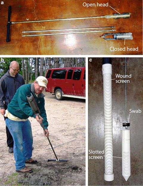

  

  Hand auger for removing sediment prior to installation of a water-table monitoring well. (a) Auger head, rod, and handle with two rod extensions and an additional auger head; (b) Augering a hole with the bucket inverted for removal of sediment; (c) PVC wound well screen, PVC slotted well screen, and well-screen swab. Note the two different types of fittings at the end of the well screen (standard PVC cap and cone-shaped PVC point). If the slotted screen is inverted and the cap is attached to the opposite end, the non-slotted interval becomes the sump

• Associated couplings and caps and PVC cement

• Bucket auger and associated hardware (8.9-cm (3.5-in.) diameter is common)

• Supply of medium sand (approximately 5-L but amount will vary depending on the diameter of the augered hole relative to the diameter of the monitoring well)

• Shovel

• Tamping rod (handle of the shovel or unused sections of auger rod can suffice)

• Hand saw

• Sledge hammer

• Tape measure or folding rule

• Water-level measurement device (e.g., chalked-steel tape, electric tape)

• Notebook, hand lens, sediment-sample bags

First, select a location for installation of the water-table monitoring well. The well should be located so that it is representative of conditions along a specific reach or area of the wetland. Criteria that are commonly considered when locating a water-table well include topographic gradient, vegetative cover, aspect, geology and soil type. Once the location is selected, use a shovel to remove the vegetation from an approximately 0.25-m² area surrounding the intended well site. Note the vegetative cover and organic soil type and thickness.

Install an appropriate auger head on a section of rod (Fig. 3.42a) (closed-head for sand and loosely consolidated sediment, open-head for cohesive sediment) and begin turning the auger in a clockwise direction until the auger bucket is full. Remove the bucket from the hole and shake or push the sediment out of the auger head (Fig. 3.42b), allowing the sediment to fall onto a clean surface, such as a board or tarp. Record the depth of the hole with a tape measure. Describe the sediment in the field notebook. Place a sample from the auger in a sample bag for later lab analysis of percent organic matter and grain-size distribution. Repeat this process until you reach the water table or the intended depth. As you auger deeper, you may need to add one or more rod extensions to the soil-auger assembly. You also may encounter large rocks that inhibit continued augering. Persistence will sometimes get you past a rock or rocky layer, but you also may have to abandon the hole and try again a short distance away.

The water table may not necessarily be obvious if the permeability of the sediment is small enough that water does not readily flow into the auger hole. In some cases, squeezing the sediment with your hand can indicate whether the sediment is saturated or not. If the sample was removed from below the water table, water will be released from the sediment as you squeeze the sample. In settings where the sediment is sandy and poorly cohesive, it is likely that saturated sediment will slump back into the hole as sediment below the water table is removed. The common solution to this problem is persistence. Keep augering through this sediment with strong downward force on the auger handle. You may need to change to an auger head that has solid sides and a narrower opening between the cutting fins so that loose, wet sand is better retained when the auger is pulled from the hole. The hole below the water table will gradually deepen as you continue to remove sediment and the loose slurry occupying the hole will become less and less dense as you continue to remove sediment from the hole. Once the desired depth has been reached, commonly about 1–1.5 m below the water table, it is time to assemble and install the well.

Record the total depth of the hole by marking the auger rod at the point where it is even with land surface when the auger is at the bottom of the hole. Remove the auger from the hole and measure the distance from the mark to the bottom of the auger. Add a distance, commonly 0.6–1 m, for the extent of the well casing that will be above the ground. This is often called the “stickup.” The sum of these distances will be the total length of the monitoring well. Assemble the well screen by gluing a cap to the bottom of the well screen and a coupling to the top of the screen (Fig. 3.42c). If available, it is desirable to use a well cap that either is cone shaped or that has the same outer diameter as the well screen to reduce resistance when pushing the assembly into the loose sediments below the water table. The well screen should be sized to be long enough that the water table is usually within the screened interval of the well. The slot size (the width of the openings in the screen) should be selected so that most of the sediment cannot pass through the well screen.

Well screens often have an interval at the bottom of the screen that does not have any slots. This is called the sump, or the volume below the screen where fine sediments that pass through the screen can accumulate without blocking the well-screen openings. Be sure to record the presence of a sump and indicate the length of the sump. This information will be important in determining the precise screened interval of the well. The existence of a sump becomes particularly important if the water table is below the bottom of the screened interval. Measurements of depth to water will indicate an erroneous water level equivalent to the elevation of the bottom of the well screen because water will be trapped in the sump. Drilling small holes in the bottom of the sump prior to well installation may allow trapped water to drain from the sump if the well goes dry.

Cut the PVC casing so that the total well length is the distance of the hole depth plus the desired stickup length. If the hole is relatively deep, you may need to attach another PVC coupling and another length of well casing to reach the desired total assembly length. By now, the sediment in the auger hole may have settled and solidified and it may be necessary to remove several additional buckets full of recently slumped sediment from the hole. Keep removing sediment from the hole until the auger has reached the bottom of the hole and the sediment is once again poorly consolidated. At this point it is important to move rather quickly, especially in sediments that readily slump and solidify, such as medium to fine sand. As soon as the last bucket of sediment is pulled out of the hole, immediately shove the completed well casing and screen into the hole and push it down until it stops. You may need to pound lightly on the top of the well casing with the sledge hammer to drive the well to the intended depth. It is prudent to place a board or drive cap on the well casing to prevent damage to the top of the well casing. While pounding lightly, grab the well casing and push downward, essentially vibrating the well downward through the loose sediment. In most cases, you will be able to reach or get very near the desired well depth. Once the well is in place, it is a simple matter of filling the annular space between the edge of the augered hole and the well casing with sediment that was removed from the hole. Tamp the sediment repeatedly as you fill the hole so the sediment is tightly consolidated. This will prevent any preferential flow of water along the outside of the well casing during recharge events. If unused segments of auger rod are used for this purpose, place duct tape over the end of the rod to prevent damage of the threads.

If the sediment is sufficiently cohesive that the augered hole remains open below the water table, inserting the completed well screen and casing is as simple as placing the assembly into the auger hole. In this case, you will then need to pour sand coarser than the well-screen slot size down the hole so that it surrounds the entire screened interval. This backfill, often called a sand pack, will ensure that the well screen does not become clogged with fine-grained sediment that otherwise would be situated next to the well screen. Once sufficient sand is added to fill the annular space to just above the screened interval, material removed from the auger hole can be added to fill the remainder of the augered hole. As described before, this sediment should be tamped to ensure that the density of the sediment filling the annular space is not less than the undisturbed material. It is common to add soil to create a small mound of soil at the base of the well that will direct rainfall away from the well casing.

Now all that is left is to install a well cap, install well protection, and make several measurements. A well cap can be as simple as a plastic slip cap that stays on the casing via friction and gravity. You might instead wish to glue on an assembly that has a threaded cap or that allows access to the well to be protected with a keyed lock. In either case, make sure that the well cap can easily be removed from the casing for measurements of depth to water. Shallow monitoring wells are not well anchored to the soil because of the smaller contact area with the soil that surrounds the well casing. Some wells can easily be moved, even in an attempt to remove a firmly attached well cap, which may change the vertical positioning of the top of the well and introduce error in determinations of hydraulic gradient. A small hole also may be drilled through the well casing to facilitate equilibration of the pressure inside of the well casing with changes in atmospheric pressure. If air cannot readily enter the well casing, the position of the water table inside of the well may not represent the water table.

In many areas, regulations require some form of protection that will minimize the chance of the well casing being inadvertently broken by a falling tree or branch or a wayward automobile or lawnmower. This may entail placing a steel casing of larger diameter over the top of the well casing and into the ground (Fig. 3.41), or installation of three or four wooden or metal posts positioned so that wayward objects will strike the posts rather than the well casing (Fig. 3.41 photo inset). Lastly, make measurements of the stickup length and the distance to the bottom of the well. Survey to the top of the well casing and determine the spatial coordinates of the well with a global positioning system (GPS) or similar device.

3.1.2.1.2.2 Piezometer Installation

The piezometer will be installed in a location where the wetland bed is beneath the water surface. In this situation, the piezometer will indicate the vertical hydraulic gradient. In order to ensure that the difference in head between the piezometer screen and the wetland stage will be measurable, the screen needs to be placed a considerable distance below the sediment-water interface, often 2–3 m or more below the sediment-water interface. If the sediments are well consolidated and do not readily slump, it may be possible to use a bucket auger to create a hole in which the well screen and casing are placed, as described previously for installation of a water-table well. If augering is possible, the augered hole should not be larger than the outside diameter of the well to prevent vertical preferential flow of water along the outside of the well casing, which could alter hydraulic head at the well screen. However, in most inundated settings the sediments simply collapse into the augered hole and it is extremely difficult to auger a hole deep enough for a piezometer installation. It is much more common to drive a piezometer to depth with a well pounder or post driver. That is what we will do here. The items you will need include:

• Well screen, cap, couplings, and casing (typically steel to withstand the rigors of pounding)

• Device for driving the well and casing to the desired depth

• Cap to protect the top of the well casing

• well swab (a device to shove water through the well screen)

• bailer or pump for removing or adding water to the well

• Measuring tape

You will want to select a well diameter that is small enough to permit the driving of the well to depth but large enough to allow installation of monitoring equipment inside of the well casing, such as a pressure transducer or temperature sensors. A common diameter for these purposes is 1.9–3.2 cm (0.75–1.25 in.). Commercial well screens are preferred because of the large surface area open to the sediments, although holes or slots can be drilled or cut with hand tools to create simple screens in coarser-grained settings. If the latter option is pursued, the much smaller aggregate surface area of the holes and slots relative to a commercial well screen may result in an unacceptable response time of the well to changes in hydraulic head.

Considerable care is needed to ensure that the well screen is not clogged during installation, especially if a well screen is made by cutting or drilling holes in the well casing. To minimize this possibility, a well swab can be constructed to force water through the screen and to clean out the screened interval of the well during and following the well installation. A well swab can be as simple as a rubber washer or washers attached to the end of a metal rod (Fig. 3.42c) so that the rubber washer rubs against the side of the well casing and screen as it is pushed up and down inside of the well casing. By pushing the rod downward, water inside the well casing is forced through the screen. An upward motion pulls water through the well screen into the well casing. Repeated up and down motion generally is sufficient to remove particles that may be stuck in the screened openings, improving the connection with the aquifer sediments and reducing the time required for the head inside of the well to become representative of the adjacent saturated sediments.

Whether a post driver or well-head driver or sledge hammer is used to advance the well assembly, it should not directly strike the top of the well casing if threads are present. Doing so could deform the threads and make it impossible to attach a coupling or additional sections of casing that would otherwise allow the well screen to be driven deeper into the sediment. A drive cap or coupling should be screwed onto the threads at the top of the well casing before striking the top of the casing to drive it farther into the sediment. The drive cap or coupling should be tightened occasionally as the casing is driven into the sediment; not doing so also may result in damaged threads. It is prudent to periodically stop driving the well and swab the well to remove sediment that may have clogged the well screen. It may be necessary to pour water into the top of the well casing so the swab pushes and pulls water, and not air, through the well screen. If additional sections of pipe are required, Teflon tape or pipe dope should be used liberally, and the fittings tightened using pipe wrenches, to ensure that no leaks occur at the junctions between pipe segments. Once the well is driven to depth, it should be thoroughly developed by repeatedly swabbing the well and screen, including periodic removal of water and suspended sediment from the well with a pump or bailer, until the water level inside the well casing recovers readily to the static water level. Once this occurs, the well is considered developed and is functioning as a piezometer.

After well installation and development you will want to measure and record:

• 1. Distance from the top of casing to the well bottom,

• 2. Distance from top of casing to the wetland bed,

• 3. Screened interval, sump interval (if present), and

• 4. Distance from the water surface to the wetland bed.

With these values determined, the distance from the sediment-water interface to the mid-point of the screened interval can be calculated. Commonly referred to as l in the Darcy equation (or sometimes l _v to indicate that the gradient is distributed on a vertical axis), this is the distance that the head difference is divided by to determine the vertical hydraulic gradient. The head difference can easily be determined by measuring the distance from the top of casing to the wetland water surface and subtracting the distance from the top of casing to the water surface inside of the well. For a small-diameter well completed in low-permeability sediments, measurements of depth to water can be corrupted if a portion of the measuring device needs to be immersed in the water to make a measurement. The volume of the sensor device immersed in the water will cause the water level to rise inside of the well. Low-permeability sediments will not permit the water level inside the well to return to static equilibrium in a sufficiently short time, resulting in a false depth-to-water measurement. Care should be taken to prevent this possibility by using a measurement method that does not require immersion of a large sensor relative to the well-casing diameter during a water-level measurement. The cut-off end of a chalked-steel tape is a particularly good device for this purpose because the volume of the steel tape immersed to make a measurement is very small.

Once the piezometer is installed, GPS coordinates and well-top elevations are determined, and measurements are made to determine the hydraulic gradient. Sensors also can be installed to continuously monitor hydraulic head, and temperature at one or more depths, inside of the piezometer (Fig. 3.41).

3.1.2.2 Field Activity 2: Single-Well Response Test

In Field activity 1, a piezometer was installed either on the margin of or beneath a wetland bed. Figure 3.43a demonstrates a piezometer in a wetland with the screen (slotted portion in the bottom) in direct contact with the sediments, and panel b demonstrates a piezometer completed in a dry margin of a wetland (the water table is below the ground surface). The latter has been installed in an augered hole with a sand pack around the screen and a clay seal above to prevent “short-circuiting” of water through the annular space. A horizontal line beneath an inverted triangle is a commonly used symbol to indicate surface-water level. This symbol is displayed here to indicate the pond water level in (a) and the water table in (b), as well as the undisturbed water levels (also called static head) in the piezometers.

Fig. 3.43

Schematic diagrams of piezometers with screen length L and radius R without (a) and with (b) a sand pack; (c) example of the plotted recovery of a single-well response test conducted in a piezometer located in Wetland 109 in the St. Denis National Wildlife Area

A single-well response test, often referred to as a slug test, is initiated by changing the water level in a water-table well or piezometer very quickly (within a few seconds) and monitoring the recovery of the water level from the initial disturbed value to the static level. A number of methods are available for creating this near-instantaneous water-level change (Butler 1998). The easiest method is to quickly lower a solid cylinder (typically made of metal or high-density plastic) attached to a length of rope into the piezometer. This solid “slug” displaces a known volume of water as it is rapidly lowered into place and the slug remains stationary for the duration of the test. The water level in the well returns to the static level at a rate that is controlled by the hydraulic conductivity of the porous medium around the well screen. After the static level is reached, a second test can be initiated by rapidly removing the cylinder, thereby causing an instantaneous drop of the water level. It is always good practice to conduct two response tests (positive and negative displacement) and check the consistency of results.

Water level is monitored during the slug test using either a manual water-level sounder or a pressure transducer, depending on the rate of water-level recovery. For low-permeability settings, manual measurements can often be made quickly enough to capture the initial rapid phase of water-level recovery and can easily be made frequently enough during the slower phase of recovery. A pressure transducer is a far better choice for wells installed in sand or coarser sediments where the entire recovery can be completed in a matter of seconds. The transducer is suspended prior to the test at a depth greater than the reach of the slug to avoid damage to the transducer, and early enough that the well has recovered to the static water level following displacement of water during immersion of the transducer. The combined length of the slug and rope needs to be carefully measured to ensure that the slug does not slam into the pressure transducer as it is rapidly lowered into the well. If the slug is completely submerged during deployment, the known slug-displacement volume can be used to estimate the initial rise (or drop) of the water level during the test. Calculation of the maximum water-level change can then be compared with the measured value. A substantial difference between calculated and measured water-level change may indicate a procedural problem or a problem with the piezometer construction. It also is important to ensure that the piezometer water level does not go below the top of the screen or the top of sand pack during the entire test. For this reason, single-well response tests are not recommended for water-table wells.

The average (or bulk) hydraulic conductivity (K _b , m s⁻¹) of the material surrounding the piezometer screen (or sand pack, if present) can be estimated from the recorded water-level data:

$$ {K_b}={{{\pi {r^2}}} \left/ {{\left( {F{T_b}} \right)}} \right.} $$

(3.66)

where r (m) is the radius of the inside of the well casing, F (m) is a shape factor representing the dimension and geometry of the groundwater flow field around the screen, and T _b (s) is the basic lag time of the piezometer (see below for definition). The “sample volume” of this method is approximately equal to a sphere with a radius similar to the length of the well screen, L (m). F is a function of L and R, the radius of the outer surface of the well screen or the sand pack, if present. Numerous equations have been suggested to estimate F for different types of piezometers under different conditions (see Butler 1998). In most cases, if L/R is not substantially smaller than 4, the formula of Hvorslev (1951) as cited by Freeze and Cherry (1979:341) gives a convenient means to approximate F:

$$ F = {{{2\pi L}} \left/ {{ \ln \left( {{L \left/ {R} \right.}} \right)}} \right.} $$

(3.67)

T _b is determined by plotting head versus time on a semi-logarithmic plot (Fig. 3.43c). For convenience, head is normalized as:

$$ {H \left/ {{{H_0}={{{\left( {h-{h_s}} \right)}} \left/ {{\left( {{h_0}-{h_s}} \right)}} \right.}}} \right.} $$

(3.68)

where h (m) is measured head, h ₀ (m) is the water level immediately after the introduction of the slug, and h _s (m) is the static water level prior to introduction of the slug. Once a straight line is fitted to the data, T _b is determined as the time in seconds since the beginning of the introduction of the slug when H/H ₀ equals 0.37 (≅ e ⁻¹) (Fig. 3.43c).

Once the slug test data have been collected and entered in a spreadsheet, you should follow the procedure listed below:

• 1. Prepare a data table containing time in one column (t = 0 at the maximum h value following introduction of the slug) and h in the second column corresponding to each value of t.

• 2. Compute H/H ₀ for each reading.

• 3. Plot H/H ₀ versus t, using a logarithmic axis for H/H ₀.

• 4. Fit a straight line to the data points, and determine the value of t where the straight fitted line crosses ${H \left/ {{{H_0}=}} \right.}0.37$. Em shows an example, in which T _b  ≅ 1,930 s.

• 5. From T _b and the dimensions of the piezometer, compute K _b .

• 6. In the example shown in Fig. 3.43c, the piezometer is constructed similarly to panel b and has dimensions of L = 0.73 m, R = 0.075 m, and r = 0.016 m. Substituting these values and T _b into Eqs. 3.66 and 3.67 gives ${K_b}=2.1\times 1{0^{-7 }}\mathrm{ m}\ {{\mathrm{ s}}^{-1 }}$. This test was conducted in a piezometer located in Wetland 109 in the St. Denis National Wildlife Area in Saskatchewan, Canada (see Hayashi et al. 1998 for details).

References

Butler JJ (1998) The design, performance, and analysis of slug tests. Lewis, Boca Raton

Freeze RA, Cheery JA (1979) Groundwater. Prentice-Hall, Englewood Cliffs

Hayashi M, van der Kamp G, Rudolph DL (1998) Water and solute transfer between a prairie wetland and adjacent uplands, 1. Water balance. J Hydrol 207:42–55

3.1.2.3 Field Activity 3: Installation of a Seepage Meter and Temperature Sensors

The use of multiple methods to determine flow between groundwater and surface water is always a good idea because it improves understanding of the physical setting and it provides independent values representative of multiple spatial scales. Field activities 1 and 2 demonstrated measurement of hydraulic gradients and hydraulic conductivity to determine Q. Field activity three provides two additional methods for determining Q. A seepage meter makes a direct measurement of Q, but over a very small portion of the wetland bed. The piezometer that we installed in the wetland can serve double duty if we suspend temperature sensors inside of the piezometer casing, allowing calculation of Q based on temperature gradients and attenuation of diurnal cycles in temperature with depth.

3.1.2.3.1 Seepage Meter Construction and Installation

What you will need:

• 208-L (55-gal) plastic storage drum

• Hand saw for cutting plastic drum

• Permanent marker

• Measuring device

• Power drill (battery-powered or electric)

• Drill bits appropriately sized for the hose-connection hardware

• Hose-connection fittings

• Rubber or cork stopper

• Plastic tub and lid to serve as a seepage bag shelter

• Plastic seepage bag (approximately 3–5 L)

• Tube and fittings to connect plastic bag to hose

• Hose to connect bag shelter to seepage cylinder

• Brick or suitable weight to place on top of seepage cylinder

A seepage meter can be made from many different readily available products. The standard “half-barrel” seepage meter is described as such because it was made by cutting the ends off of a standard 208-L (55-gal) storage drum (Lee 1977). Although many other cylinders have been used as seepage meters, such as coffee cans, cut-off trash cans, trash-can lids, even wading pools, the half-barrel meter is often used because it is rigid, durable, does not readily deform, covers a larger surface area than many of the other devices, is still quite inexpensive, and can be easily obtained from many industrial supply companies. A storage drum will be used in this exercise. First, obtain a storage drum from one of a large number of suppliers. Either metal or plastic drums can be used, but to simplify construction for this exercise, you should obtain a plastic drum. Be sure to order a closed-top drum to eliminate possibilities of leaks associated with an open-top drum where the top can be removed, and order the larger 208-L (55-gal) drum because it covers a larger surface area than the 114-L (30-gal) drum. You will make seepage cylinders from the top and the bottom thirds of the drum.

Mark the side of the drum a consistent distance from one end of the barrel; commonly, a length of 30–35 cm is used. Connect the dots (marks) by drawing a line along the circumference of the drum. Use the hand saw to cut along this line to remove one end from the drum. Repeat this process for the other end of the drum. If vegetation on the wetland bed is tall and dense, you may instead simply cut the barrel in half, essentially making two seepage cylinders, each approximately 45 cm tall. A cross-cut hand saw can be used to cut the plastic drums whereas a cutting torch or reciprocating saw (or a hack saw used with great persistence) are generally required to cut a metal barrel. Carefully measure the diameter or the circumference of the open end of the cut-off cylinder and calculate the area based on either measurement. This open end of the cylinder will equal the area of the wetland bed covered by the seepage cylinder. Most 208-L drums will cover an area of about 0.25 m².

Next, you will need to drill a hole in the side of the drum, near the drum end, to which a short hose will be attached (Fig. 3.44). The short hose will extend from the seepage cylinder to a seepage-bag shelter that will protect the bag from wind and waves, curious animals, and diving ducks (Fig. 3.45). The diameter of the hole will depend on the hardware that you use to attach the hose to the seepage cylinder. There are many different options available. Water flows through a seepage meter under very low pressure. The fitting should not leak under small pressures but you do not need to go to the expense of installing a water-tight bulkhead fitting either. Lastly, drill a small hole approximately 0.5–1 cm in diameter at the highest point of the seepage cylinder (vent hole identified in Fig. 3.1). This will be the vent for releasing any gas that is trapped during seepage-meter deployment. This hole will be open during installation of the seepage cylinder and then plugged with a rubber or cork plug during operation. If substantial amounts of gas are generated, a common situation in many wetland settings, you may need to install a vent tube that will extend above the water surface so that gas can be released to the atmosphere during seepage-meter operation (Lee and Cherry 1978).

Fig. 3.44

Half-barrel seepage cylinder showing ports installed both in the top and the side of the cylinder. A section of garden hose with female garden-hose connectors on both ends (not shown) is used to connect the bag shelter to the seepage cylinder

Fig. 3.45

Half-barrel seepage meter installed in sandy sediment. Note side port, to which the hose is connected, and top port with cap and vent hole with rubber stopper

The seepage bag, used to measure the volume of water that flows across the sediment-water interface covered by the seepage cylinder, also can be made from a variety of materials. A convenient bag volume is 3–4 L and thin-walled, flexible bags are preferable. Lightweight freezer-storage bags have often been used. Avoid using bags with thicker walls, such as medical intravenous (IV) bags or solar-shower bags; these bags have a substantial resistance to expansion and contraction in response to being filled or emptied. Use of these bags will substantially reduce the volume of water that otherwise would flow across the bed covered by the seepage cylinder. The opening of the bag can be gathered together around a hose and taped to the hose so the fitting does not leak. Another option is to weld or otherwise seal the bag opening and cut a small slit in one of the corners of the bag, through which you will insert a hose or tube and tape the bag to the hose or tube. As with the seepage cylinder, the bag and fittings should not leak under small pressures but the assembly does not withstand large pressures. It is convenient to install hardware that includes a valve that can be closed while the bag is being transported, attached or removed from the seepage cylinder, and during subsequent handling prior to being weighed or measured.

The bag should be placed in a shelter for several reasons: (1) to prevent the bag from being exposed to currents, (2) to maintain the bag in a proper orientation, and (3) to protect the bag from fish or mammals or waterfowl, a particularly important consideration in many wetland settings. Many different types of bag shelters have been used; examples are provided in Figs. 3.44 and 3.45. Design and build a bag shelter of your choosing, including a section of tubing or hose that will connect to the side opening on the seepage cylinder. The hose or tubing should be approximately 1–2 m long, which ensures that you will not disturb the seepage cylinder while attaching or removing the seepage-collection bag.

3.1.2.3.1.1 Seepage-Meter Installation

Select a location near the piezometer that you installed as part of field activity 1. Wade to the location, making sure to not step on the area that will be covered by the seepage cylinder. The bed should not be covered by any large rocks or debris (i.e., waterlogged sticks) that would alter seepage or prevent insertion of the seepage cylinder. Make sure the rubber plug is removed and the port on the side of the seepage cylinder is open; this allows water to escape as you are pressing the seepage cylinder into the wetland sediments. Press the cylinder into the sediment very slowly, allowing gas and water to escape through the top vent tube. You may need to twist the cylinder to aid in cutting through a vegetative mat, if one is present. If aquatic vegetation is very dense you may need to first cut a slit in the vegetative mat with a long knife to facilitate insertion of the cylinder. The bottom rim of the cylinder typically needs to penetrate the sediment approximately 5–10 cm to ensure a good seal with the sediment. However, if the bed surface is uneven, the insertion depth may need to be increased so no gaps are present beneath the edge of the seepage cylinder. You should probe with your fingers along the interface between the wetland bed and the seepage cylinder. If you can feel the bottom edge of the cylinder, then the insertion depth is not sufficient. In this case, press the cylinder deeper into the sediment until you can no longer feel the bottom edge of the cylinder. The meter also should be inserted with a slight tilt so that the vent hole is at the highest point, allowing any gas released from the sediment to escape. Once the meter is set, place a weight on the meter to counter the buoyant force of the plastic material. A concrete or masonry brick usually is sufficient. Plug the vent tube with the rubber stopper. The stopper will be removed later, prior to seepage measurement, to provide a relative guide for the volume of gas released from the sediment. If the volume is substantial, you will want to install a vent tube to release gas to the atmosphere. If unvented, gas released from the sediment will collect inside of the seepage cylinder, displacing water that will be routed to the seepage-collection bag.

Install the bag shelter and connect the shelter to the seepage cylinder. You may also need to place a small weight inside of the bag shelter to hold it in place and prevent movement in response to waves. The wetland bed has been substantially disturbed during meter installation and it is common for seepage rates to be larger than normal following meter installation. It is common practice to wait for hydraulic conditions at and near the bed to stabilize before measuring seepage. If your field schedule permits, wait until the next day before making the first measurement, or measure seepage directly after installation and compare those values with measurements made the following day.

3.1.2.3.1.2 Seepage-Meter Measurement

Since you do not know whether water is flowing into or from the wetland across the portion of the wetland bed isolated by the seepage cylinder, start your first measurement with the seepage bag approximately half filled with water. Place a known volume of water inside of the bag. Volume can be determined either with a graduated cylinder or by weighing the water and the bag with an electronic scale. If using an electronic scale, knowing that the density of water is 1 g/cm³and that 1 ml equals 1 cm³ allows you to measure change in volume by recording change in weight of the seepage bag. Before making any measurements using an electronic scale, you should weigh the bag empty, then completely full, so you will know the range of volume that can be measured with the bag.

Once an initial volume of water in the bag has been measured (or weighed), you will need to remove all remaining air from inside of the bag prior to connecting the bag to the seepage cylinder. This is commonly called de-airing the bag. Close the valve on the bag that contains a measured volume of water, walk out to the bag shelter, suspend the bag vertically while holding onto the bag fitting, open the valve, and slowly lower the bag into the water, immersing the bag with the valve constantly pointing up and always above the water surface. This process will force air inside of the bag to leave via the open valve located above the water surface. Once the bag is pulled beneath the surface to the point where water inside of the bag is at the same level as the valve, close the valve. The bag is now de-aired and ready for deployment.

Carefully remove the bag-shelter lid and attach the bag to the threaded fitting inside of the bag shelter. Straighten the bag so the bag material is not twisted and the bag is oriented in a relaxed position inside of the bag shelter. Open the valve and record the time of opening. Your measurement has begun. Place the lid on the bag shelter very slowly to avoid forcing water out of the bag during the measurement. Now you wait. Since you do not know the seepage rate a priori, the wait time is somewhat of a guessing game. A half hour to an hour should be sufficient to allow a change in water volume that is large enough to allow you to know whether water is flowing to or from the bag. To remove the bag, repeat the process described above but in reverse. Remove the lid on the bag shelter very slowly, and close the valve on the bag being careful to not touch the bag. Record the time as you close the valve. Remove the bag and measure the final volume of water (or determine the final weight of the bag plus water if an electronic scale was used prior to bag attachment). By the gain or loss in volume or weight, you will know the direction of flow and have an initial assessment of the relative seepage rate. If the bag is full or empty upon removal, you waited too long and your next measurement should be conducted over a shorter period. If there is no measurable change in volume, your next measurement period should be increased. After one or two iterations, you should have a good estimate for the amount of time it will take to make a seepage measurement. Simply divide the change in volume by the time of bag attachment to get seepage results in ml/min. Divide that value by the area covered by the seepage cylinder to report your results in flux units (distance per time).

3.1.2.3.2 Installation of Temperature Sensors

Accurate measurements of temperature can be made easily with inexpensive instruments, making its use in quantifying exchanges between groundwater and surface water particularly attractive. Here we will make use of newer technology for measuring temperature, along with the concepts presented in Sect. 3.6, to determine a value for Q at the piezometer we installed earlier. This value can be compared to Q determined with the Darcy method described in Field activity 1.

Two basic types of electronic sensors are commonly deployed for this purpose. The thermocouple is a device that consists of two wires made of different metals that are connected together at both ends. A current is generated when two junctions of these wires are exposed to different temperatures. Copper and constantan wires are commonly paired for use in environmental applications. The method requires that one of the junctions be related to a known temperature. Therefore, a separate reference temperature sensor also is required to use this measurement method. The second commonly used sensor, and one that often is used as the reference thermometer for thermocouple installations, is the thermistor. A thermistor is basically a resistor that changes resistance in response to changing temperature. The choice of thermocouple or thermistor often depends on the number of temperature sensors required. If more than 5–10 sensors are required, it may be more cost effective to deploy thermocouples.

Two methods of deploying temperature sensors also commonly are used. One consists of a sensor connected to wires that transmit the signal to a nearby data-collection device (Fig. 3.46), and the other consists of the sensor and datalogger in a single, self-contained unit. Recent versions of the latter device have become very small (e.g., 17 mm diameter) and can be inserted inside small-diameter piezometers.

Fig. 3.46

Nest of piezometers installed at different depths beneath the wetland bed with pressure transducers and temperature sensors installed in five of the seven wells. All sensors are connected to a digital datalogger positioned on shore to the left of the photo. Note also the four seepage meters, with bags attached directly to the tops of the seepage cylinders, installed near the wells. Attaching the bag directly to the seepage cylinder is sometimes acceptable where wind and currents are minimal

Either type of sensor can be used for this installation. First, familiarize yourself with the electronic thermometer of choice, making sure that the sensor output is reasonable, that output changes in response to placing the sensor in a warmer or colder environment, and the sensor is logging data. For this application, collecting data at 15-min intervals generally is sufficient to monitor diurnal changes in temperature, although more frequent data collection is certainly acceptable.

Attach one sensor to the outside of the casing of the piezometer that is installed in standing water in the wetland. The sensor should be positioned just above the sediment-water interface. You may also wish to deploy an additional sensor to record changes in air temperature that drive changes in the wetland water temperature. Next, position one sensor at the bottom of the well and another one or two sensors at equal distances between the well bottom and the sediment-water interface. Only one sensor is actually required to be deployed inside of the well; additional sensors allow a determination of the degree of heterogeneity in hydraulic conductivity between the sediment-water interface and the bottom of the well. It is common to suspend sensors on appropriate lengths of string or fine wire from the top of the well (be sure to first check whether the sensors sink or float), or if a signal cable is involved, to affix the signal cable to the top of the well so the sensor hangs at the appropriate depth.

Collect data from the sensors for a period of one to several weeks. Retrieve the sensors, download the data, and plot the time series from all sensors on the same plot.

• 1. After viewing the data you have collected, is it likely that groundwater is discharging to the wetland or that wetland water is flowing vertically downward to become groundwater? Or is it not possible to make this determination based on your data?

• 2. Calculate the difference between the daily maximum and minimum temperatures for each sensor. Plot the differences versus time. If you have collected air-temperature data, include daily differences for air temperature as well. Can you make any determination regarding any potential change in the rate of flow across the sediment-water interface?

You can determine the rate of vertical flow across the wetland bed in either direction using the methods described in Short exercise 11. You will also need estimates of thermal conductivity, porosity, dispersivity, and heat capacity of the sediment. Since you also know the vertical hydraulic-head gradient based on measurements you made at this piezometer in field activity 1, you could use one of several methods described in Appendix B of Stonestrom and Constantz (2003) to determine Q. As an additional exercise, you are encouraged to use the free software described in Stonestrom and Constantz to calculate Q based on the temperature data you have collected.

References

Lee DR (1977) A device for measuring seepage flux in lakes and estuaries. Limnol Oceanogr 22:140–147

Lee DR, Cherry JA (1978) A field exercise on groundwater flow using seepage meters and mini-piezometers. J Geol Educ 27:6–20

Stonestrom DA, Constantz J (2003) Heat as a tool for studying the movement of ground water near streams: U.S. Geological Survey Circular 1260:96

3.1.2.4 Field Activity 4: Stream Gaging Techniques

Stream inflow or outflow may be the dominant component of a wetland water balance, in which case it is important to measure stream discharges as accurately as possible. The following field activities will provide values of stream discharge using three different methods. These measurements are ideally conducted in a relatively small stream with a well-defined channel that is safely accessible by observers.

First, identify a suitable stream reach that satisfies the conditions listed in the first paragraph of the “Discharge measurement” segment of Sect. 3.4. Following the procedures described in “Velocity-area-method” of Sect. 3.4, a measurement section perpendicular to the flow direction should be set up. One observer wades into the stream with a current meter and a device to measure the depth of water (e.g., a wading rod), while the second observer takes notes on the bank and also takes necessary precautions for the safety of the observer in the stream. Depending on the type of current meter used, the velocity is measured at a prescribed depth (e.g., six-tenth point for the Price-type meter), or averaged over the entire depth profile in a subsection. From the depth and velocity data for individual subsections, the total discharge is calculated using Eq. 3.22. Repeat the same measurement two or three times, preferably moving the cross section upstream or downstream by several meters, and compare the results to assess the repeatability and errors of the method.

Next, measure discharge in the same stream reach using the float method described in the section “Other methods of discharge measurement”. This method usually is not as accurate as the velocity-area method, but it provides a useful alternative when a current meter is not available. Any floating objects that are clearly visible and are relatively unaffected by wind can be used. Subsections should be determined in a manner similar to the velocity-area method (but usually with coarser spacing of measurement points). Once points are determined, float-velocity measurements simply replace measurements made with a current meter. The profile-averaged velocity can be estimated by multiplying the surface velocity determined with the floats by 0.85.

The tracer-dilution method provides a third value of stream discharge at this stream reach. First, select a suitable location upstream of the measured cross section for release of the stream tracer. This location should be sufficiently far upstream to ensure complete mixing of the tracer solution. This may require preliminary release of tracer at several upstream locations, along with accompanying downstream measurements of tracer concentration at several locations, to confirm complete mixing. You will want to select a tracer that can be released in small quantities but that will not be masked by the background concentration in the stream. The tracer also needs to be one that is not regulated by any stream-management authorities, or one for which you have a permit to release.

It may be convenient to use electrical conductivity (EC) as a surrogate for tracer concentration if a sufficient amount of tracer can be released to create an easily measured increase of the EC of the stream water. In streams that have very low background EC, a strong correlation between tracer concentration (e.g., chloride) and EC can be pre-established, and concentration can be estimated from the measurements of EC. If this is not feasible, water samples will need to be collected and analyzed with a field analyzer or in the laboratory. This will require a large number of samples for slug injection tests.

After the location for tracer release is selected, a choice must be made between the constant-rate injection (CRI) and the slug injection (SI) method. The CRI method requires a device for injecting tracer solution at a constant rate, but only three values of concentration are required (see Eq. 3.23). The SI method does not require a special device, but many concentration values are required to establish the time-concentration curve shown in Fig. 3.17. Here we describe the use of the CRI method. It is assumed that the background concentration is small enough that the tracer concentration can be estimated from the measurement of EC. To establish the relation between EC and tracer concentration, prepare a set of standard solutions from the tracer chemical and the stream water; for example, solutions of 0, 5, 10, 20, … 1,000 mg of sodium chloride in 1 L of stream water. The EC values of these solutions are plotted against concentration values to establish a calibration curve.

For successful application of the CRI method, the tracer solution should be released at an appropriate rate and concentration to ensure that concentration at the measurement section can be accurately measured relative to the stream background concentration, and that a sufficient volume of tracer solution exists in the tracer-injection reservoir to achieve steady state at the sampling location. The constant release rate of tracer solution can be maintained using a Mariotte bottle or a field-portable pump with controlled flow rate (see Moore 2004 for construction of a simple Mariotte bottle from readily available materials). Once a steady value of EC is established at the sampling location and tracer concentrations are determined, the observer can calculate discharge using Eq. 3.23.

In summary, the suggested field activities for stream gauging are the following:

• 1. Determine stream discharge using the area-velocity method. If time permits, determine the discharge at multiple locations and assess the errors and uncertainty of this method.

• 2. Estimate stream discharge using the float method at the same location, and compare the accuracy of this method with the area-velocity method.

• 3. Determine stream discharge using the tracer dilution method.

• 4. Compare the values of discharge obtained by all three methods and discuss their advantages and disadvantages for application at this particular location, as well as other possible locations and situations.

References

Abtew W (2001) Evaporation estimation for Lake Okeechobee in south Florida. J Irrig Drain Eng 127:140–147
Adams DD (1994) Sediment pore water sampling. In: Mudrock A, MacKnight (eds) Handbook of techniques for aquatic sediments sampling. Lewis Publishers, Boca Raton
Allan MA (2004) Manual for the GAW precipitation chemistry programme: guidelines, data quality objectives and standard operation procedures. World Meteorological Organization Global Atmosphere Watch No. 160:170
Allen RG, Pereira LS, Raes D, Smith M (1998) Crop evapotranspiration – guidelines for computing crop water requirements. Food and Agricultural Organization of the United Nations FAO Irrigation and drainage paper 56:328
Belanger TV, Kirkner RA (1994) Groundwater/surface water interaction in a Florida augmentation lake. Lake Reserv Manag 8:165–174
Bouwer H (1989) The Bouwer and Rice slug test – an update. Ground Water 27:304–309
Bouwer H, Rice RC (1976) A slug test for determining hydraulic conductivity of unconfined aquifers with completely or partially penetrating wells. Water Resour Res 12:423–428
Brooks R (2009) Potential impacts of global climate change on the hydrology and ecology of ephemeral freshwater systems of the forests of the northeastern United States. Clim Chang 95:469–483
Brunsell NA, Ham JM, Owensby CE (2008) Assessing the multi-resolution information content of remotely sensed variables and elevation for evapotranspiration in a tall-grass prairie environment. Remote Sens Environ 112:2977–2987
Brutsaert WH, Stricker H (1979) An advection-aridity approach to estimate actual regional evapotranspiration. Water Resour Res 15:443–450
Carr MR, Winter TC (1980) An annotated bibliography of devices developed for direct measurement of seepage. U.S. Geological Survey Open-File Report 80-344:38
Choi J, Harvey JW (2000) Quantifying time-varying ground-water discharge and recharge in wetlands of the northern Florida Everglades. Wetlands 20:500–511
Conly FM, Su M, van der Kamp G, Millar JB (2004) A practical approach to monitoring water levels in prairie wetlands. Wetlands 24:219–226
Constantz J, Niswonger R, Stewart AE (2008) Analysis of temperature gradients to determine stream exchanges with ground water. In: Rosenberry DO, LaBaugh JW (eds) Field techniques for estimating water fluxes between surface water and ground water. U.S. Geological Survey Techniques and Methods 4-D2, Denver, pp 117–127
Cunningham WL, Schalk CW (2011) Groundwater technical procedures of the U.S. Geological Survey. U.S. Geological Survey Techniques and Methods 1-A1:151
Dalton MS, Aulenbach BT, Torak LJ (2004) Ground-water and surface-water flow and estimated water budget for Lake Seminole, northwestern Georgia and northwestern Florida. U.S. Geological Survey Scientific Investigations Report 2004-5073:49
Dingman SL (2002) Physical hydrology. Prentice-Hall, Upper Saddle River
Doss PK (1993) Nature of a dynamic water table in a system of non-tidal, freshwater coastal wetlands. J Hydrol 141:107–126
Drexler JZ, Snyder RL, Spano D, Paw UKT (2004) A review of models and micrometeorological methods used to estimate wetland evapotranspiration. Hydrol Process 18:2071–2101
Dunne T, Leopold LB (1978) Water in environmental planning. W.H. Freeman and Company, New York
Elsawwaf M, Willems P, Feyen J (2010) Assessment of the sensitivity and prediction uncertainty of evaporation models applied to Nasser Lake, Egypt. J Hydrol 395:10–22
Euliss NH Jr, LaBaugh JW, Fredrickson LH, Mushet DM, Laubhan MK, Swanson GA, Winter TC, Rosenberry DO, Nelson RD (2004) The wetland continuum: a conceptual framework for interpreting biological studies. Wetlands 24:448–458
Ferré PA, Topp GC (2002) Time domain reflectometry. In: Dane JH, Topp CC (eds) Methods of soil analysis part 4 – physical methods. Soil Science Society of America, Madison