
Abstract
This extended chapter of almost hundred pages on black hole physics is a central part of the book. We begin with Israel’s original demonstration of the statement that a static black hole solution of Einstein’s vacuum equation has to be spherically symmetric, and is thus a Schwarzschild black hole. Then a detailed derivation of the Kerr solution is given, that makes efficient use of Cartan’s calculus of differential forms. The properties of this rotating black hole solution, that ranks among the most important solutions of Einstein’s (vacuum) equations, are carefully analysed, and it is shown in a more general setting what is behind the results. Later, this is also used in derivations of the four laws of black hole dynamics, which are formally closely related to the main laws of thermodynamics. A section is devoted on accretion tori around Kerr black holes. Furthermore, we present the evidence for black holes in some X-ray binary systems and for supermassive black holes in galactic centres.
Access this chapter
Tax calculation will be finalised at checkout
Purchases are for personal use only
Notes
- 1.
- 2.
Since the last edition of this book, the situation has improved. Under the assumption that a stationary, axisymmetric vacuum solution has a Killing horizon (defined in Sect. 8.4.4), it was constructively shown that it is the Kerr solution [253]. The explicit construction, based on the “inverse scattering method” for solutions of certain boundary value problems, provides thus at the same time a nice uniqueness proof for stationary axisymmetric black holes. This result was recently extended to the Kerr–Newman family [254] (including the case of a degenerate horizon).
- 3.
This can be seen as follows:
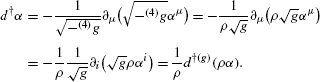
Alternatively, d † α=d †(g) α−〈dlnρ,α〉.
- 4.
The Riemannian mapping theorem guarantees always the existence of a holomorphic diffeomorphism (conformal transformation) between two simply connected domains D 1 and \(D_{2}\not=\mathbb{C}\). In general the mapping f:D 1⟶D 2 does not extend to a homeomorphism of \(\bar{D}_{1}\) onto \(\bar{D}_{2}\). If the boundary of D 1 is a finite union of smooth curves, one can show that f extends to a homeomorphism \(f:\bar{D}_{1}\longrightarrow\bar{D}_{2}\) (see, e.g., [59], Proposition 6.2).
- 5.
In a first step we can choose z such that it is orthogonal to ρ: γ=e2h(dρ 2+f dz 2). Since ρ is harmonic, one readily concludes that f is independent of ρ. By a simple redefinition of z we can, therefore, choose f≡1.
- 6.
For a precise formulation and a complete proof we refer to [280]. Unfortunately, so far the unjustified hypothesis of analyticity of the metric in a neighbourhood of the event horizon had to be made.
- 7.
For certain matter models, for instance for source-free electromagnetic fields, this exhausts all stationary black holes (circularity and staticity theorems).
- 8.
Note that k is tangent to the static limit since by (8.220) L k 〈k,k〉=0. If the normal would be null, then it would be proportional to k, but then it could not be perpendicular to m, except at the poles (where the normal is actually null).
- 9.
By this one means that \(\mbox{det}(\partial^{2}S/\partial q^{\mu}\partial\alpha_{\nu})\not=0\). Such solutions always exist locally.
- 10.
- 11.
Active galactic nuclei produce prodigious luminosities in tiny volumes (in some cases as much as 104 times the luminosity of a typical galaxy in much less than 1 pc3). This radiation can emerge over an extraordinarily broad range of frequencies. For a text book presentation of active galactic nuclei, see e.g. [281].
- 12.
Perform, if necessary, a transformation of the coordinates x A in (8.72).
- 13.
There are various ‘physical’ and mathematical formulations of the cosmic censor conjecture (see, e.g., [9]). Since nothing has been proven about the validity of the conjecture, we do not discuss this issue.
- 14.
Consider a linear map J:ℝ2⟶ℝ2, y=J x. In ℂ this reads \(w=\bar{a} z+b \bar{z}\), where z=x 1+ix 2, w=y 1+iy 2 and
$$\bar{a}=\frac{1}{2}(J_{11}+J_{22})- \frac{i}{2}(J_{12}-J_{21}) , \qquad b=\frac{1}{2}(J_{11}-J_{22})+\frac{i}{2}(J_{12}+J_{21}) . $$We see that
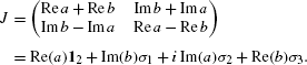
Note that detJ=|a|2−|b|2, \(\operatorname{Tr} J=2 \operatorname{Re} a\).
- 15.
Note that the orthogonal complement of T p S in T p M is a two-dimensional Minkowski vector space. Hence it contains two different null directions, an “ingoing” and an “outgoing” one.
- 16.
- 17.
In [9] the spacetime (M,g) is said to be strongly asymptotically predictable, if in the unphysical spacetime \((\tilde{M},\tilde{g})\) there is an open region \(\tilde{V}\) containing the closure of
 in \(\tilde{M}\), such that \((\tilde{V},\tilde{g})\) is globally hyperbolic.
 - 18.
This means that H is a topological manifold with an atlas whose transition functions are locally Lipschitz.


 in
in References
Textbooks on General Relativity: Selection of (Graduate) Textbooks
R.M. Wald, General Relativity (University of Chicago Press, Chicago, 1984)
G. Ellis, S. Hawking, The Large Scale Structure of Space-Time (Cambridge University Press, Cambridge, 1973)
C.W. Misner, K.S. Thorne, J.A. Wheeler, Gravitation (Freeman, New York, 1973)
N. Straumann, General Relativity and Relativistic Astrophysics. Texts and Monographs in Physics (Springer, Berlin, 1984)
Textbooks on General Physics and Astrophysics
V.I. Arnold, Mathematical Methods of Classical Mechanics. Graduate Texts in Mathematics, vol. 60 (Springer, Berlin, 1989)
Mathematical Tools: Modern Treatments of Differential Geometry for Physicists
R. Abraham, J.E. Marsden, Foundations of Mechanics, 2nd edn. (Benjamin, Elmsford, 1978)
Mathematical Tools: Selection of Mathematical Books
B. O’Neill, Semi-Riemannian Geometry with Applications to Relativity (Academic Press, San Diego, 1983)
M.E. Taylor, Partial Differential Equations (Springer, New York, 1996)
Research Articles, Reviews and Specialized Texts: Chapter 4
R. Schödel et al., Nature 419, 694 (2002). astro-ph/0210426
Research Articles, Reviews and Specialized Texts: Chapter 7
R. Schoen, S.-T. Yau, Commun. Math. Phys. 90, 575 (1983)
Research Articles, Reviews and Specialized Texts: Chapter 8
W. Israel, Phys. Rev. 164, 1776 (1967)
W. Israel, Commun. Math. Phys. 8, 245 (1968)
M. Heusler, Black Hole Uniqueness Theorems (Cambridge University Press, Cambridge, 1996)
M. Heusler, Stationary black holes: uniqueness and beyond. Living Rev. Relativ. 1, 6 (1998). http://www.livingreviews.org
M.S. Volkov, D.V. Gal’tsov, Phys. Rep. 319, 1–83 (1999)
R.P. Kerr, Phys. Rev. Lett. 11, 237 (1963)
E.T. Newman, A.I. Janis, J. Math. Phys. 6, 915 (1965)
E.T. Newman et al., J. Math. Phys. 6, 918 (1965)
G.C. Debney et al., J. Math. Phys. 10, 1842 (1969)
G. Neugebauer, R. Meinel, J. Math. Phys. 44, 3407 (2003)
R. Meinel, arXiv:1108.4854
R.D. Blandford, R.L. Znajek, Mon. Not. R. Astron. Soc. 179, 433 (1977)
K.S. Thorne, R.H. Price, D.A. MacDonald, Black Holes: The Membrane Paradigm (Yale University Press, New Haven, 1986)
N. Straumann, The membrane model of black holes and applications, in Black Holes: Theory and Observation, ed. by F.W. Hehl, C. Kiefer, R.J.K. Metzler (Springer, Berlin, 1998)
N. Straumann, Energy extraction from black holes, in Recent Developments in Gravitation and Cosmology, ed. by A. Macias, C. Lämmerzahl, A. Camacho. AIP Conference Proceedings, vol. 977 (American Institute of Physics, New York, 2008). arXiv:0709.3895
B. Carter, Commun. Math. Phys. 10, 280 (1968)
J.M. Bardeen, W.H. Press, S.A. Teukolsky, Astrophys. J. 178, 347 (1972)
M. Heusler, N. Straumann, Class. Quantum Gravity 10, 1299 (1993)
M. Heusler, N. Straumann, Phys. Lett. B 315, 55 (1993)
V. Iyer, R.M. Wald, Phys. Rev. D 50, 846 (1994)
R.M. Wald, Phys. Rev. D 56, 6467 (1997). gr-qc/9704008
R.M. Wald, Black holes and thermodynamics, in Black Holes and Relativistic Stars, ed. by R.M. Wald (University of Chicago Press, Chicago, 1998)
B. Carter, J. Math. Phys. 10, 70 (1969)
B. Carter, Black hole equilibrium states, in Black Holes, ed. by C. DeWitt, B.S. DeWitt (Gordon & Breach, New York, 1973)
D.R. Gies, C.T. Bolton, Astrophys. J. 304, 371 (1986)
A.P. Cowley et al., Astrophys. J. 272, 118 (1983)
J.E. McClintock, R.A. Remillard, Astrophys. J. 308, 110 (1986)
J.A. Orosz, Inventory of black hole binaries, in IAU Symposium No. 212: A Massive Star Odyssey, from Main Sequence to Supernova, Lanzarote, 2002, ed. by K.A. van der Hucht, A. Herraro, C. Esteban (Astronomical Society of the Pacific, San Francisco, 2003). astro-ph/0209041
R.M. Wagner et al., Astrophys. J. 556, 42 (2001)
J.E. McClintock et al., Astrophys. J. 551, L147 (2001)
M. Miyoshi, J. Moran, J. Herrnstein, L. Greenhill, N. Nakai, P. Diamond, M. Inone, Nature 373, 127 (1995)
T. Ott et al., ESO Messenger 111, 1 (2003). astro-ph/0303408
M. Kozlowski, M. Jaroszynski, M.A. Abramowicz, Astron. Astrophys. 63, 209 (1978)
M. Sikore, M. Jaroszynski, M.A. Abramowicz, Astron. Astrophys. 63, 221 (1978)
D. Giulini, J. Math. Phys. 39, 6603 (1998)
P.T. Chrusciel, E. Delay, G. Galloway, R. Howard, Ann. Inst. Henri Poincaré 2, 109 (2001)
P.T. Chrusciel, Helv. Phys. Acta 69, 529 (1996)
J.H. Krolik, Active Galactic Nuclei (Princeton University Press, Princeton, 1999)
Ch.J. Willott, R.J. McLure, M. Jarvis, Astrophys. J. 587, L15 (2003)
R. Penrose, Structure of spacetime, in Battelle Rencontres: 1967 Lectures in Mathematics and Physics, ed. by C. DeWitt, J.A. Wheeler (Benjamin, New York, 1968)
R. Genzel et al., Nature 425, 934 (2003)
M.J. Valtonen et al., Nature 452, 851 (2008)
Author information
Authors and Affiliations
Appendix: Mathematical Appendix on Black Holes
Appendix: Mathematical Appendix on Black Holes
1.1 8.8.1 Proof of the Weak Rigidity Theorem
In this section we prove the weak rigidity theorem quoted in Sect. 8.4.4, making use of the notation and tools developed in Sect. 8.3.1. For convenience, we repeat its formulation
Theorem 8.3
(Weak rigidity theorem)
Let (M,g) be a circular spacetime with commuting Killing fields k, m and let Ω=−〈k,m〉/〈m,m〉, ξ=k+Ωm. Then the hypersurface H={〈ξ,ξ〉=0}, assumed to exist, is null, and Ω stays constant on H. The null surface H is thus a Killing horizon.
Proof
First, we establish that H is a null hypersurface. For this we introduce
where
Note that H is given by σ=0. Conceptually it is clear that the hypersurfaces {σ=const} are invariant under the isometry group ℝ×SO(2), so that the vector fields k and m are tangent to these surfaces. Analytically, this follows from
and similar equations. Therefore the gradient ∇σ is perpendicular to k and m, i.e., ∇σ∈E ⊥, where E is the integrable distribution spanned by the vector fields k and m. Below we establish that on H the gradient ∇σ is also in E. Thus ∇σ| H ∈E∩E ⊥. This intersection is one-dimensional on H, and generated by the null field ξ. (Verify that ξ∈E ⊥ on H.) Hence the normal ∇σ of H is null, proving that H is lightlike.
Let us now calculate the gradient of σ. We have
Here we use

to get
Now, we multiply this equation from the right with (k∧m), and use in the resulting expressions the Frobenius conditions (see (8.70)). These and the anti-derivation rule for the interior product imply, for example
Collecting terms gives
Especially on H we get dσ∧(k∧m)=0. At this point we make the generic assumption that the group action is such that k and m are linearly independent on H. Then dσ must be a linear combination of k and m.—In [266] it is shown that the non-degeneracy assumption just mentioned is not necessary, but this requires more work.
The second part of the theorem, Ω| H =:Ω H =const follows with a similar argument. Let us look at the gradient of Ω. As before ∇Ω∈E ⊥. On the other hand we find in a first step
The same manipulations which led to (8.347) give now, using i ξ k=〈ξ,ξ〉 and i ξ m=〈ξ,m〉=0,
On H the right-hand side vanishes, and we again reach the conclusion that ∇Ω∈E, thus ∇Ω is proportional to ξ. In other words ∇Ω is normal to H, hence H is a surface of constant Ω. This completes the proof. □
1.2 8.8.2 The Zeroth Law for Circular Spacetimes
We consider the same situation as in Appendix 8.8.1. The strategy for proving that κ is constant on a Killing horizon will be similar to the one we used in proving the constancy of Ω| H .
We extend the definition of the surface gravity κ outside the horizon in a natural manner by (see (8.292))
Since k and m are commuting Killing fields, we have
and L m 〈dl,dl〉=0. Therefore the gradient ∇κ is in E ⊥. Below we show that it is on H also in E, so ∇κ has to be proportional to l. This implies that κ on H is a constant.
Once we have established that
we are done. To show this we start from the following consequence of the two Frobenius conditions (8.70)
which holds everywhere. Taking the interior product with l gives
On this we apply d∘i Z for any vector field Z and obtain

In the next step we show that when this equation is restricted to H the first three terms vanish. For the first term this is clear, since both factors in the parenthesis vanish on H. (Recall that the twist of l vanishes on H.) Obviously the third term is also zero on H. To show this for the second term we have to consider (N:=〈l,l〉)
which vanishes on H since dN is proportional to l and l∧dl| H =0. So we arrive at
As above, we have

So the factor of m in (8.352) is equal to

In (8.352) we need the restriction of this to H. The first two terms in the last expression obviously vanish there, and in the third term we can replace dN by −2κl. So (8.352) becomes
Is it allowed to replace dN in the last expression also by −2κl, in spite of the exterior differentiation? The answer is yes, as the following simple argument shows. After multiplication with (−2κ) the last term in the square bracket of (8.353) has the form dN∧df for a function f. If we again use adapted coordinates, with N one of them, and {x i} parameterizing H, we have \(df=\bar{d}f+\partial_{N}f\,dN\), where \(\bar{d}f=\partial_{i}f\,dx^{i}\) is the differential in H. So \(dN\wedge df=dN\wedge\bar{d}f\) on H, showing that on H dN∧df=dN∧dg for two functions f and g that agree on H. Therefore, on H
and (8.353) becomes
Since the vector field Z is arbitrary, we arrive at (8.350).
Let us summarize: On a Killing horizon, whose outer domain of communication is circular, the surface gravity is constant. This is the zeroth law for circular spacetimes.
Note that this is a purely geometrical fact. We have never used the field equations and no assumptions on the matter content had to be made. The proof of the zeroth law for static spacetimes is left as an exercise.
Exercise 8.6
Prove the zeroth law for a Killing horizon, whose outer domain of communication is static.
Hints
For a static spacetime with Killing field K, we have K∧dK=0. Apply on this d∘i Z ∘i K and restrict the result to the Killing horizon to conclude that K and ∇κ are proportional.
1.3 8.8.3 Geodesic Null Congruences
Congruences of timelike geodesics of a Lorentz manifold have been studied in Sect. 3.1. In this appendix we investigate the behaviour of (infinitesimal) light beams. We shall introduce the “optical scalars” and derive their propagation equations. This material is indispensable for proving the area law. Some of it will also be used in the proof of the positive energy theorem for black holes (see Chap. 9). Null congruences also play an important role in the proofs of singularity theorems.
Consider a light beam with wave vector field \(k=\dot{\gamma}\). Let γ(λ) be a central null geodesic, and consider a one-parameter family of neighbouring null geodesics of the beam, i.e., a variation of γ in the sense of DG, Sect. 16.4, with deviation vector field X along γ. As shown in DG, Sect. 16.4, X satisfies the Jacobi equation
where a dot denotes the covariant derivative ∇ k in the direction k. Note that

because of the symmetry properties of the Riemann tensor. So 〈k,X〉 is a linear function of λ. Note also that along γ(λ) fields of the form \((a\lambda+b)\dot{\gamma}(\lambda)\), with a, b constants, are Jacobi fields. Subtracting such a tangent field changes the scalar products of X with timelike vector fields (e.g. velocity fields), but leaves the scalar product with k unchanged. In the eikonal limit deviation vectors which connect rays contained in the same phase hypersurface satisfy
This property holds for the equivalence class of deviation vectors that differ from X by multiples of k. As in the timelike case (Sect. 3.1), the deviation vectors of such a class simply correspond to different parametrisations of neighbouring geodesics. For null congruences the scalar product of two deviation vectors obviously depends only on their equivalence classes. This simple fact is physically important (e.g. in gravitational lensing). In what follows we shall assume that (8.355) holds.
1.4 8.8.4 Optical Scalars
We choose a four-velocity field u along the central ray γ, which is parallel along γ and satisfies 〈u,u〉=−1. Furthermore, we normalize the affine parameter λ such that 〈k,u〉=−1.
Let us now introduce the following basis along γ: E A , for A=1,2, is an orthonormal basis of the plane orthogonal to the span of k and u, which is parallel along γ. We also use the complex vector ε=E 1+iE 2 and its conjugate complex \(\bar{\varepsilon}=E_{1}-i E_{2}\). The following scalar products are obvious,

Let us also take
Then {E 0,…,E 3} form an orthonormal vierbein along γ.
Next, we introduce the optical scalars θ, σ and ω defined by
where
Thus we have
1.5 8.8.5 Transport Equation
The vector field X can be decomposed as
(A priori we can write X=(ξ 1 E 1+ξ 2 E 2)+(ξ 0 E 0+ξ 3 E 3), but 〈X,k〉=0 implies ξ 0=ξ 3, hence the last term is proportional to k.) Also let
thus
Note that by (8.356)
hence, recalling that k and X commute,
where we used that \(\nabla_{k}X=\nabla_{X}k=\frac{1}{2}\xi \nabla_{\bar{\varepsilon}}k+\frac {1}{2}\bar{\xi}\nabla_{\varepsilon}k+0\). The resulting transport equation
is important in what follows. The real form of this equation is easily derived.Footnote 14 Let
then
where

From (8.368) the geometrical meaning of the optical scalars in obvious:

because the optical deformation matrix S splits as

(In the literature θ is often defined to be the trace of S.)
We remark that if k is a gradient field, then k α;β =k β;α , hence
which is equivalent to ρ being real, that is ω=0. (See also Eq. (8.374) below.)
Next we show that
From the definition of θ we have

Now, the metric can be decomposed as follows

or
where the first term is the induced metric on span{E 1,E 2}. Thus
If this is inserted in (8.371) and use is made of

we obtain indeed
We leave it as an exercise to show similarly that
Hence, the rotation rate ω vanishes if dk=0. (For a more general condition, see the applications below.) Derive also an invariant expression for |σ|2 in terms of covariant derivatives of k (consider for this k (α;β) k (α;β)).
1.6 8.8.6 The Sachs Equations
We now give a very simple (possibly novel) derivation of the propagation equations for the optical scalars. We start by differentiating the transport equation (8.365):

On the other hand, the Jacobi equation (8.354) gives

Identifying like terms, we obtain (\(\mathcal{R}\) is real, see below)


We rewrite \(\mathcal{R}\) and \(\mathcal{F}\):

giving
Similarly, we find
Here, because of (8.356) only the Weyl tensor C αμβν contributes (see Sect. 15.10 for the definition of the Weyl tensor),
Let us split (8.376a) into two equations for the real and imaginary parts. Together with (8.376b) we get the basic Sachs equations for the propagation of the optical scalars:


Of particular importance is (8.380a), also known as the Raychaudhuri equation.
Let us write the Jacobi equation (8.375), i.e.,
also in real form:
where the optical tidal matrix T is given by

Conceptually, one should regard ξ as a representative of the “equivalence class mod k” of X (see (8.361)).
1.7 8.8.7 Applications
Let us consider some special families of null geodesics that play an important role in GR, for instance in proofs of singularity theorems.
First, we consider a spacelike two-dimensional surface S in the spacetime (M,g) and a congruence of null geodesics orthogonalFootnote 15 to S for some neighbourhood U⊂S. Let k denote the tangent vector field (or the corresponding one-form), and let {E i ,i=1,2} be an orthonormal basis of vector fields of S in U. We choose a point p∈U and the null geodesics γ with γ(0)=p (see Fig. 8.11).—We claim that for this situation the rotation rate ω vanishes at p, for any p∈U.

Two-parameter family of null geodesics normal to a two-dimensional spacelike surface S
The proof of this is simple. From the definition one sees thatFootnote 16
On the initial surface S, where 〈E 1,k〉=〈E 2,k〉=0, the Ricci identity gives
since [E 1,E 2]∈TS (see DG, Appendix C).
If the initial value of ω vanishes, the propagation equation (8.380c) implies that ω=0 everywhere. So the two-parameter family sketched in Fig. 8.11 has vanishing rotation.
Consider next a congruence of null geodesics which is orthogonal to a family of hypersurfaces, the wave fronts, as in the eikonal approximation of wave optics. According to the Frobenius theorem, this is locally equivalent to (see DG, (C.24))
In the notation introduced above, we evaluate k∧dk on the triple \((\varepsilon,\bar{\varepsilon},u)\). Using the scalar products in (8.356), and the definition of ρ, we get

This shows that ρ is real, hence ω=0.
For ω=0 the Raychaudhuri equation (8.380a) for the expansion θ becomes particularly interesting, because the right-hand side of
is non-positive if some reasonable energy condition is assumed. Indeed, Einstein’s field equation implies
and this is non-negative if the following weak energy condition
for all timelike ξ μ is satisfied. In this case (8.387) implies

or, integrating between λ 0 and λ,
So if θ(λ 0) is negative, θ(λ) will become unboundedly negative in the interval [λ 0,λ 0−θ(λ 0)−1]. This means that the area element between neighbouring curves of a two-parameter variation as in Fig. 8.11 goes to zero somewhere in this interval (see Eq. (8.400) below). The point on the null geodesic where this happens is a focal point (or conjugate point) of S along the null geodesic.
Let us summarize this important conclusion.
Proposition 8.1
Let θ be the expansion rate along a null geodesic whose initial rotation rate ω vanishes. If the weak (or strong) energy condition for the energy-momentum tensor holds, then θ(λ 0)<0 implies that θ becomes −∞ at a finite value of the affine parameter λ in the interval [λ 0,λ 0−θ(λ 0)−1], provided the null geodesic is defined on this interval. This holds, in particular, for any geodesic of a hypersurface orthogonal congruence of null geodesics, and for a two-parameter family of null geodesics normal to a two-dimensional spacelike surface.
1.8 8.8.8 Change of Area
We come back to the situation sketched in Fig. 8.11. The two-parameter family of null geodesics defines the one-parameter family of immersions

for some interval of λ. Let η λ be the induced volume forms on ϕ λ (U). We want to know how these change with increasing λ. As expected, the rate for this is twice the expansion rate θ:
For deriving this we need the fact that k is orthogonal to the family of immersed submanifolds ϕ λ (U). This one may call “Gauss’ lemma for null geodesics” (see Sect. 3.9). To prove it, let σ(t) be a curve in U, and consider the one-parameter subfamily of null geodesics starting on σ(t):λ↦F(λ,t)=ϕ λ (σ(t)). The tangential fields along F belonging to ∂/∂λ and ∂/∂t are
Obviously, V is tangential to the submanifolds ϕ λ (U). To show that 〈k,V〉=0 we consider
So \(\frac{\partial}{\partial\lambda}\langle k,V\rangle=0\). Since for λ=0, k and V are orthogonal, k is orthogonal to all surfaces ϕ λ (U).
It will be useful to introduce an orthonormal frame {E α } which is adapted to the foliation: E i (i=1,2) are tangential to the submanifolds ϕ λ (U), and E A (A=0,3) are normal to ϕ λ (U). The dual basis of 1-forms is denoted by {θ α}. Obviously,
We want to compute
Let Θ=θ 1∧θ 2, then
The last term vanishes, because k is perpendicular to E 1 and E 2:
For the first term on the right of (8.394) we use the first structure equation, giving (\(\omega_{\;\beta}^{\alpha}\) denote the connection forms)

Hence,
On the other hand we have, using the notation ε α ≡〈E α ,E α 〉=±1,
Therefore, the mean curvature normal
where ⊥ denotes the normal component, can be expressed as (ε j =1)
Hence
Comparison with (8.395) gives
so
This proves (8.392), since by (8.384) and (8.396)
Here, the scalar product on the right-hand side is the so-called convergence.
A consequence of (8.392) is this: Let V⊂U, then
In particular, if θ≥0 the area of ϕ λ (V) does not decrease. On the other hand, if θ were negative somewhere along one of the null geodesics, Proposition 8.1 implies that one could find a neighbourhood V such that the area of ϕ λ (V) vanishes at some finite value of λ (provided that the null geodesic is defined on a sufficiently large interval). This will play an important role in the next section.
From (8.400) and (8.392) we obtain for the first and second derivatives of the area \(\mathcal{A}_{\lambda}\) of ϕ λ (V)


For an infinitesimal \(\mathcal{A}_{\lambda}\) this gives, together with the Raychaudhuri equation (8.387),
This formula finds, for instance, also applications in cosmology (angular distance).
1.9 8.8.9 Area Law for Black Holes
If the spacetime (M,g) satisfies certain general conditions (global hyperbolicity and asymptotic predictabilityFootnote 17) the horizon H is a closed embedded three-dimensional C
1−-submanifoldFootnote 18 (see Proposition 6.3.1 in [10]), and is generated by null geodesics without future endpoints. (Null geodesic generators of null hypersurfaces are introduced in DG, Appendix A. Note that null geodesic through a point of H is unique, up to rescaling of the affine parameter.) Null geodesic generators may leave H in the past, but have to go into  . Such leaving events are called caustics of H. At a caustic H is not C
1 and has a cusp-like structure. But once a null geodesic has joined into H it will never encounter a caustic again, never leave
H
and not intersect any other generator. All these properties, established by R. Penrose in [283], are (partially) proved in a pedagogical manner in [15], Box 34.1. There is no point to repeat this here.
. Such leaving events are called caustics of H. At a caustic H is not C
1 and has a cusp-like structure. But once a null geodesic has joined into H it will never encounter a caustic again, never leave
H
and not intersect any other generator. All these properties, established by R. Penrose in [283], are (partially) proved in a pedagogical manner in [15], Box 34.1. There is no point to repeat this here.
Based on these properties we now “prove” the area law (the second law) for black holes. If the horizon were a sufficiently smooth submanifold, the area law would follow easily. Using the differential geometric tools developed in the previous Appendix 8.8.3, we could argue as follows.
Consider two Cauchy hypersurfaces Σ and Σ′, with Σ′ in the future of Σ, and let \(\mathcal{H}=H\cap \varSigma \) and \(\mathcal{H}'=H\cap \varSigma '\) be the horizons at time Σ, respectively Σ′. We want to compare the surface areas
where \(\eta_{\mathcal{H}}, \eta_{\mathcal{H}'}\) denote the induced volume forms (measures) on \(\mathcal{H}\) and \(\mathcal{H}'\). At each point \(p\in\mathcal{H}\) there is a unique future- and outward-pointing null direction perpendicular to \(\mathcal{H}\), and we can choose a vector field l of future directed null vectors. (Show that this is possible in a smooth fashion.) The null geodesics with these initial conditions, i.e., the family
are generators of H without future endpoints. Therefore, they intersect Σ′ in unique points on \(\mathcal{H}'\), with unique affine parameter τ(p) for each \(p\in\mathcal{H}\). If we rescale the null field l as k(p):=τ(p)l(p), then we obtain a injective map

(The map Φ is in general not surjective because new generators may join the horizon.) As in Appendix 8.8.3 we introduce the one-parameter family of immersions

for λ∈[0,1]. Clearly, Φ=ϕ λ=1.
From Proposition 8.1 we conclude that the expansion rate θ (or the negative of the convergence) of the generating family of null geodesics, λ↦ϕ λ (p), \(p\in\mathcal{H}\), cannot be negative, if the weak energy condition of matter holds. (Otherwise focal points would be formed in the future, violating Penrose’s theorem on the global structure of horizons (quoted above).) Formula (8.401) then implies that
Unfortunately, this beautiful argument is based on a smoothness assumption for the horizon that is generally not satisfied, because of the formation of caustics where the manifold has a cuspy structure. As was pointed out by several authors, the general validity of the area law is for this reason still an open problem. For discussions of this delicate issue, that appears somewhat strange from a physical point of view, we refer to [278] and [279].
Exercise 8.7
Derive (8.374) and show that
Rights and permissions
Copyright information
© 2013 Springer Science+Business Media Dordrecht
About this chapter
Cite this chapter
Straumann, N. (2013). Black Holes. In: General Relativity. Graduate Texts in Physics. Springer, Dordrecht. https://doi.org/10.1007/978-94-007-5410-2_8
Download citation
DOI: https://doi.org/10.1007/978-94-007-5410-2_8
Publisher Name: Springer, Dordrecht
Print ISBN: 978-94-007-5409-6
Online ISBN: 978-94-007-5410-2
eBook Packages: Physics and AstronomyPhysics and Astronomy (R0)