
Abstract
This chapter concerns portfolio optimization, which is one of the historically first problems in financial mathematics. Indeed, one of the basic problems that a given subject (physical person or institution), possessing a certain amount of wealth, has to deal with is the following: how to invest this wealth in the financial market over a given period of time in order to be able to consume optimally (according to a given criterion) from this portfolio over time and at the end have a residual amount leading to benefit, also this one optimal according to a given criterion. The optimality criterion that we shall consider is the most common one, namely the maximization of expected utility of the various monetary amounts.
Access this chapter
Tax calculation will be finalised at checkout
Purchases are for personal use only
Notes
- 1.
1Since we are interested in the utility maximization problem, putting u(v) = −∞ for v ∈ ℝ \ I is equivalent to excluding values outside the interval I from being optimal.
- 2.
2Recall that by our assumptions a≤ 0 and 1 + r> 0.
- 3.
3For a full proof see for example Proposition 2.7.2 in [7].
- 4.
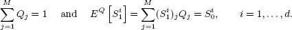
For example, in the one-period case, assuming for simplicity r = 0, we havethat \( Q\in {\mathbb{R}}_{+}^M \) is a martingale measure if
- 5.
5The inequality “≥” is obvious. To show the inverse inequality, fix ε> 0 and consider functions η ε N , …, η ε N such that

Then, in the mean, we obtain
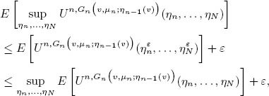
from which the thesis follows, given the arbitrariness of ε.
- 6.
6It holds, furthermore, that C max N (υ) = υ.
- 7.
It holds, furthermore, that C maxN (v) = v.
- 8.
It holds, furthermore, that C maxN (v) = v.
- 9.
If V n–1 = 0 then V n ≤ K for any π n ∈ ℝ
- 10.
M can be computed explicitly as in (2.129).


Author information
Authors and Affiliations
Rights and permissions
Copyright information
© 2012 Springer-Verlag Italia
About this chapter
Cite this chapter
Pascucci, A., Runggaldier, W.J. (2012). Portfolio optimization. In: Financial Mathematics. Unitext(). Springer, Milano. https://doi.org/10.1007/978-88-470-2538-7_2
Download citation
DOI: https://doi.org/10.1007/978-88-470-2538-7_2
Publisher Name: Springer, Milano
Print ISBN: 978-88-470-2537-0
Online ISBN: 978-88-470-2538-7
eBook Packages: Mathematics and StatisticsMathematics and Statistics (R0)