
Abstract
We experimentally explore how investor decision horizons influence the formation of stock prices. We find that in long-horizon sessions, where investors collect dividends till maturity, prices converge to the fundamental levels derived from dividends through backward induction. In short-horizon sessions, where investors exit the market by receiving the price (not dividends), prices levels and paths become indeterminate and lose dividend anchors; investors tend to form their expectations of future prices by forward, not backward, induction. These laboratory results suggest that investors’ short horizons and the consequent difficulty of backward induction are important contributors to the emergence of price bubbles.
The original article first appeared in Journal of Economic Dynamics and Control 31:1875–1909, 2007. A newly written addendum has been added to this book chapter.
Access this chapter
Tax calculation will be finalised at checkout
Purchases are for personal use only
Notes
- 1.
- 2.
- 3.
Allen et al. (1993) argue that even in markets with long-term investors the backward induction can fail and bubbles form when investors do not know others’ expectations.
- 4.
When subjects were recruited, they were told to participate in an experiment in market decision-making for 2–3 h in total. At the beginning of the session in a laboratory, subjects knew that (i) they had already spent about an hour and half for instruction and trial sessions, and (ii) one period was three minutes long followed by the paper work for a minute or two. Thus they could predict that the session would end well before period 30.
- 5.
Other variations are also possible. An announcement that the terminal dividend would be paid at period 30 but the session will end earlier, say at period 15, for sure, would break the link completely. Alternatively, the session could be terminated with a common knowledge probability distribution to retain a weak but well-specified link. For example, we could have announced that there will be a ten percent chance that the session will be terminated at the end of period 10, 11, 12, 13, or 14, with the predicted price payoff; if the session goes to period 15, it will be terminated with the pre-specified dividend payoff.
- 6.
One may wonder whether the average predicted price (liquidation value) may be a candidate for fundamental value in the short-horizon sessions. This predicted price, however, cannot be considered as the fundamental value because the prediction is, itself, endogenous to the market process that includes the behavior of investors and predictors. No concept of value that deserves the label of fundamental can properly be a function of such behavior because then the label itself becomes superfluous.
- 7.
Biais and Bossaerts’ (1998) model shows this possibility.
- 8.
We adopted relative performance based payment in Sessions 8–11 due to limitations of our budget. In the absolute performance based payment sessions, payment to subjects when a bubble arises could be considerable. For example, in session 2, we paid 138 dollars per subject on average for a 3 h session. We changed the payment policy from absolute to relative for the subsequent short-horizon sessions.
- 9.
The average prices were calculated by excluding transaction prices that result from order-of-magnitude typographical errors (8 transactions in total throughout 11 sessions).
- 10.
We had different subjects play the two roles to avoid confounding the incentives of the investors and the predictors.
- 11.
We conjecture that in Session 3, a bubble formed because at least some of the subjects did not fully understand the instructions about the structure of the security. In period 4 the price rose to 320, although the subjects knew that the maximum possible dividend in this market was only 300. In period 15, one subject sold shares at a price of 1; he later told us that he forgot that the securities earned a liquidating dividend at the end of the last period. In Session 5 (Fig. 13.3), the price dropped below the fundamental value (175) in period 15. The experimenter failed to disable the trading function on the predictors’ computers. Although the instructions prohibited predictors from trading, one of the predictors traded anyway, and 14 of the 17 trades in period 15 were sales by this predictor. We confirmed that this predictor’s trading had no significant effect on the convergence pattern to the fundamental value during the first 14 periods of the session.
- 12.
We exclude 3 transactions that resulted from order-of-magnitude typographical errors in Sessions 4 and 6, and 21 predictor’s transactions in Session 5 (see, the previous footnote) as errors, from a total of 583 transactions.
- 13.
It is possible that we did not observe bubbles in Sections 5, 6, and 7 because we did not succeed in our attempt to induce our laboratory subjects to develop divergent first and higher order beliefs about dividends. We asked the subjects “not to assume that other subjects have the same dividends as their own” and announced a range containing all investors’ dividends, which was wider than the actual distribution of dividends. We cannot rule out the possibility that this procedure does not necessarily induce divergent first and higher-order beliefs.
- 14.
Bubbles with stable prices are also suggested by Ackley (1983). He states, “…a speculative price—(i.e., a non-equilibrium price) is not always or necessarily a moving price. The price may rest for a considerable period of time at—or fluctuate narrowly around—a level far above (or below) any equilibrium determined by market fundamentals.” (p. 6)
- 15.
During period 4, when prices rose shapely, investor #5 bought 15 shares (out of 30 transactions in this period) and his cash balance went down from 11,966 to 1,353.
- 16.
To cope with heteroskedasticity, we used White’s (1980) heteroskedastic-consistent standard error to test the significance of the coefficients. Furthermore, we also run weighted least squares regressions and found that the inferences given below remained unchanged.
- 17.
In period 3 of Session 4, one predictor submitted an abnormally high price prediction (600), after observing an order-of-magnitude typographical error in a trading price in period 2. We regard this expectation data as a noise and exclude from the sample. Inclusion of this datum does not change our results.
- 18.
We thank the referee for pointing out that the possibility of session-specific effects should be considered. We re-estimated the original equations after including session dummies for long- as well as short-horizon sessions. The new estimates and their significance level are almost unchanged, with two exceptions: (i) The coefficients of (D max – P t ) for long-horizon sessions, which are significant at 1 percent level in the original estimates, have p-values of 0.063 in (13.5) and 0.064 in (13.9) when session dummy is included. Coefficients of (E t-1(P t )–P t ) and (P t-P t-1 ) are insignificant in the dummy regressions as well as the original regressions. (ii) Coefficient of (E t-1(P t )–P t ) in (13.9) for short-horizon sessions becomes significant at 5 % level in the dummy regression (p-value = 0.017) compared to 1 % level in the original regression. These results show that there is no qualitative change in our main findings after session-specific effects are controlled for.
- 19.
- 20.
The efficiency dropped just before the end of Session 3. After the session ended, a high-dividend trader who had accumulated a large number of securities told us that in period 15 he forgot that there was a terminal dividend, panicked, and sold off many securities at a price of 1.
- 21.
However, in Session 1, the efficiency rose to almost 100 percent. Since the investors could be reasonably sure that they would get the average predicted price that hovered around 83 through almost the entire session, there was no pressure for the securities to be transferred to the higher-dividend investors. In fact, 39 of the 40 securities were held by one of the two high-dividend investors at the end of Period 12. One low-dividend investor held one security, while one high-dividend and one low-dividend investor held no securities. It is therefore plausible that the transfer of securities to one high-dividend investor could have been the outcome of idiosyncratic trading strategies of the investors, and the securities could have just as easily ended up in the hands of any of the other three investors.
- 22.
Duration is the first derivative of the present value of a security with respect to the discount rate, or the weighted average time of cash flows associated with the security.
References
Ackley G (1983) Commodities and capital: prices and quantities. Am Econ Rev 73:1–16
Allen F, Gorton G (1993) Churning bubbles. Rev Econ Stud 60:813–836
Allen H, Taylor MP (1990) Charts, noise and fundamentals in the London foreign exchange market. Econ J 100:49–59
Allen F, Morris S, Postlewaite A (1993) Finite bubbles with short sale constraints and asymmetric information. J Econ Theory 61:206–229
Allen F, Morris S, Shin SH (2006) Beauty contests, bubbles and iterated expectations in asset markets. Rev Financ Stud 19:719–752
Biais B, Bossaerts P (1998) Asset prices and trading volume in a beauty contest. Rev Econ Stud 65:307–340
Blanchard O, Watson MW (1982) Bubbles, rational expectations and financial markets. In: Wechtel P (ed) Crises in the economic and financial system. Lexington Books, Lanham
De Long JB, Shleifer A, Summers L, Waldmann R (1990a) Noise trader risk in financial markets. J Polit Econ 68:703–738
De Long JB, Shleifer A, Summers L, Waldmann R (1990b) Positive feedback investment strategies and destabilizing rational speculation. J Financ 45:375–395
Dow J, Gorton G (1994) Arbitrage chains. J Financ 49:819–849
Fama EF (1991) Efficient capital markets: II. J Financ 44:1575–1617
Forsythe R, Palfrey TR, Plott CR (1982) Asset valuation in an experimental market. Econometrica 50:537–567
Frankel JA, Froot KA (1987) Using survey data to test standard propositions regarding exchange rate expectations. Am Econ Rev 77:133–153
French K, Roll R (1986) Stock market variances: the arrival of information and the reaction of traders. J Financ Econ 17:5–26
Froot KA, Scharfstein DS, Stein JC (1992) Herd on the street: informational inefficiencies in a market with short-term speculation. J Financ 47:1461–1484
Goetzmann W, Massa M (2002) Daily momentum and contrarian behavior of index fund investors. J Financ Quant Anal 37:375–389
Hirota S, Sunder S (2007) Price bubbles sans dividend anchors: evidence from laboratory stock markets. J Econ Dyn Control 31:1875–1909
Hommes CH (2006) Heterogeneous agent models in economics and finance. In: Tesfatsion L, Judd KL (eds) Handbook of computational economics, vol 2: agent-based computational economics, chapter 23, North-Holland, pp 1109–1186
Hommes CH, Sonnemans J, Tuinstra J, van de Velden H (2005) Coordination of expectations in asset pricing experiments. Rev Financ Stud 18:955–980
Jagadeesh N, Titman S (2001) Momentum. J Financ 56:699–720
LeBaron B (2006) Agent-based computational finance. In: Tesfatsion L, Judd KL (eds) Handbook of computational economics, volume 2: agent-based computational economics, chapter 24, North-Holland, pp 1187–1233
Lei V, Noussair CN, Plott CR (2001) Nonspeculative bubbles in experimental asset markets: lack of common knowledge of rationality vs. actual irrationality. Econometrica 69:831–859
LeRoy SF (2003) Rational exuberance. Mimeo
Miller M, Modigliani F (1961) Dividend policy, growth and the valuation of shares. J Bus 34:411–433
Moore R (1998) The problem of short-termism in British industry, Economic notes no. 81. Libertarian Alliance, London
Plott CR, Sunder S (1982) Efficiency of experimental security markets with insider information: an application of rational-expectations models. J Polit Econ 90:663–698
Scheinkman J, Xiong W (2003) Overconfidence and speculative bubbles. J Polit Econ 111:1183–1219
Shiller RJ (1981) Do stock prices move too much to be justified by subsequent changes in dividends. Am Econ Rev 71:421–436
Shiller RJ (2000) Irrational exuberance. Princeton University Press, Princeton
Smith VL, Suchanek GL, Williams AW (1988) Bubbles, crashes, and endogenous expectations in experimental spot asset markets. Econometrica 56:1119–1151
Stiglitz JE (1990) Symposium on bubbles. J Econ Perspect 4:13–18
Sunder S (1995) Experimental asset markets: a survey. In: Kagel JH, Roth AE (eds) Handbook of experimental economics. Princeton University Press, Princeton
Taylor MP, Allen H (1992) The use of technical analysis in the foreign exchange market. J Int Money Financ 11:304–314
Tirole J (1982) On the possibility of speculation under rational expectations. Econometrica 50:1163–1181
Tirole J (1985) Asset bubbles and overlapping generations. Econometrica 53:1499–1528
Tonello M (2006) Revisiting stock market short-termism. Conference Board, New York
White H (1980) Heteroskedasticity-consistent covariance matrix estimator and a direct test for heteroskedasticity. Econometrica 48:817–838
Williams AW (1987) The formation of price forecasts in experimental markets. J Money Credit Bank 19:1–18
Author information
Authors and Affiliations
Corresponding author
Editor information
Editors and Affiliations
Appendices
This addendum has been newly written for this book chapter.
Appendix 1: Instruction Sheets for the Subjects for Session 2
1.1 General Instructions
This is an experiment in market decision making. The instructions are simple, and if you follow them carefully and make good decisions, you will earn more money, which will be paid to you at the end of the session.
In this session, we conduct a market in which you can trade an object we shall call “shares.” You will be assigned the role of either an investor or a predictor. At the beginning of session, your role (investor or predictor) is determined by lots: “I” means investor and “P” means predictor. Your role does not change during the session.
If you are assigned to the role of an investor, you may buy/sell shares in the market. At the end of the session, your total points gained from the market will be converted into U.S. dollars at $ 0.015 per point and paid to you in cash. The more points you earn, the more dollars you will take home with you.
If you are assigned to the role of a predictor, you will predict the average market price at which the investors trade shares each period. What you earn each period depends on the accuracy of your price prediction. The more accurately you predict the share prices, the more dollars you will take home with you.
During this session, neither investors nor predictors are allowed to talk to any other participant. Also, you are to follow the various instructions given by experimenter. Violation of instructions risks forfeiting your earnings.
1.2 Investors Instructions
If you are assigned to role of an investor, you may trade shares. At the start of the session, you are given 10 shares. You may sell these shares or keep them until the end of the session. You are also provided with an initial “cash” of 10,000 points. You may use the points to purchase shares or keep them until the end of the session. Trading in shares should follow the rules to be explained later.
The session consists of many market periods of 3 min each. That is, period 1 takes place during the first 3 min of trading, period 2 in the second 3 min, period 3 in the third 3 min, and so on. The number of periods will not exceed 30.
To buy shares you should have cash to pay for them. Buying a share reduces your cash balance by the purchase price. You may sell any shares you have. Selling increases your cash balance by the sale price.
If you keep a share, then you receive a dividend on it at the end of period 30. It is written on the Dividend Card given to you before period 1. Dividend is your private information, and it may be different for different investors. You are not informed of other’s dividends. The range of dividends will be announced at the beginning of period 1.
In the likely case that the session ends before period 30, each share you hold at the end of the last period (i.e., at the end of the session) will be converted into points at the average of the predictions of the next period’s price made by the predictors.
Your profits in this experiment are the sum of profits from two sources: trading profits and end-of-session payoff. Your trading profits are equal to the change in your cash balances due to trading, which is calculated as (your cash balance at the end of last period – your initial cash provided at the beginning of the experiment). Your end-of-session payoff will depend on the number of shares you hold at the end. If the session lasts for 30 periods, this payoff will be (the number of shares you hold at that time × your dividend per share on the Dividend Card). If the session ends earlier, this payoff will be (the number of shares you hold at that time × average predicted price). Your total profits will be converted from points into U.S. dollars at the rate of $0.015 per point and paid to you in cash (Fig. 13.13).

Investor’s record sheet
1.3 Predictors Instructions
Predictors are asked to predict the prices at which the investors trade shares in each 3 min period. At the beginning of each period, you predict the average stock price of the period by writing it down in the column of My Predicted Price on your Price Prediction Sheet. We shall gather this information before starting trading for the period. At the end of each period, we shall write on the board the average predicted price for all to see.
During the period, you can see bids, asks and transaction prices on the big screen in the room.
Your profit for the period depends on the accuracy of your price prediction. Each period, you will earn 100 minus the absolute difference between your prediction and the actual trading price (averaged across all transactions in the market) shown on the big screen. For example, suppose, you predict a price of 960 and the actual average price is 980, you have a prediction error of 20 points, and your prediction earnings will be 100 minus 20 which is 80. On the other hand, if the actual average transaction price turns out to be 900, you have prediction of error of 60 points, and your prediction earnings will be 100–60 = 40.
You should record the actual average price, your prediction error (Absolute Difference), and your earning on your Price Prediction Sheet at the end of each period. At the end of the experiment, you should add your prediction earnings for all periods. Your total earnings are converted from points into U.S. dollars at the rate of $0.015 per point and paid to you in cash (Fig. 13.14).

Price prediction sheet
1.4 Instruction Set 2 (Trading Screen Operation)
-
1.
Figure 13.15 shows an active trading screen belonging to Investor 1.
Fig. 13.15 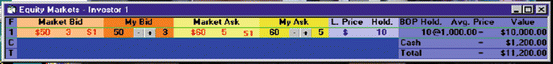
Trading screen
-
2.
Your identification number is shown in the title bar.
-
3.
The number of shares you have are shown in the light blue section under the “Hold.” label. This number increases when you buy and decreases when you sell shares.
-
4.
The clock in your CapLab screen (Fig. 13.16) starts ticking down from a preset time allowed for trading, and shows the amount of time remaining till the end of trading.
Fig. 13.16 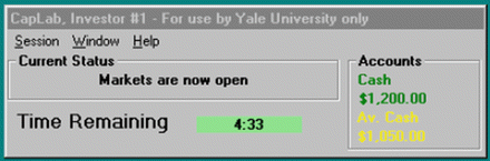
Clock
-
5.
Your cash balance is shown in the CapLab screen in green font in Fig. 13.16.
-
6.
Submit your bids (proposals to buy shares) by entering price and quantity under the “My Bid” column in brown section and pressing the enter key. Do the same for submitting asks (proposals to sell shares) under the “My Ask” column in deep yellow section. Note that default quantity is 1 share.
-
7.
When you submit a bid (proposal to buy), the computer checks if your bid price is higher than the existing market bid and if you have enough cash to pay for the purchase. If both the answers are affirmative, the market bid is replaced by your bid on the screen in the light brown section.
-
8.
When you submit an ask (a proposal to sell), the computer checks if your ask price is lower than the existing market ask and if you have the shares you propose to sell. If both the answers are affirmative, the market ask is replaced by your ask in the light yellow section of the screen.
-
9.
CapLab warns you whenever your own bid (or ask) is the market bid (or ask) by displaying them in red font on your trading screens.
-
10.
You can change your bid/ask price by one unit with each click on the plus or minus buttons.
-
11.
Please remember that your bid/ask is not submitted until you press the enter key.
-
12.
Caplab shows the identity of the investor who made the market bid/ask next to price and quantity. An S1 label under the Market Bid or Market Ask columns means investor number 1 made it.
-
13.
You can buy shares in two different ways:
-
You can submit a bid under My Bid (brown section) and wait for someone else to accept it
-
If you see a market ask price in light yellow section at which you would like to buy, submit the same price and appropriate quantity under My Bid.
-
-
14.
You can sell shares in two different ways:
-
You can submit an ask under My Ask (deep yellow section) and wait until someone to accept it.
-
If you see a market bid price (in light brown section) at which you would like to sell, submit the same price and appropriate quantity under My Ask.
-
-
15.
If bid and ask cross (bid is above ask), transaction is executed at the price equal to the bid or ask that came first.
-
16.
Whenever a transaction takes place, you will see the unit price of the latest transaction on the right hand side in the light blue section under label “L. Price.”
-
17.
This market has no book or queue. When a better one overtakes an unaccepted bid/ask, the latter is simply flushed from the system. It does not stay in the memory.
-
18.
At the end of each period, the average trading price for the period will be shown under the heading “Avg. Price” at the right end of the trading screen. You may ignore the “BOP Hold.” and “Value” columns.


Appendix 2: Supplementary Materials
Supplementary data associated with this article can be found in the online version at doi:10.1016/j.jedc.2007.01.008
Addendum: Further Analysis (Short-Horizon Session with Two Stocks)
This addendum has been newly written for this book chapter.
In short-horizon sessions of our experiment, we had a single stock to be traded in each market and observed that the price of the security was no longer anchored to its single dividend, even when it was certain and common knowledge. Price levels and changes became indeterminate; some exhibited positive bubbles of various sizes, while the one exhibited a negative bubble; some of bubbles showed some stability while the others grew rapidly. Indeterminacy seems to be an appropriate label for the great variation in the levels and changes in prices observed across sessions of the experiment.
When backward induction through time from a terminal dividend far into indefinite future generates indeterminacy, one may inquire if cross sectional induction across two or more such securities may still occur. If it does, the absolute level of prices of both the securities would be indeterminate, but the two prices will maintain a predictable relationship. To examine this proposition, we conducted a short-horizon treatment with two stocks, on November 9, 2002 at Yale University (Session A1). Stock 1 had a terminal dividend of 75 and Stock 2 had a terminal dividend of 120 and the rest of the treatment is the same as the one in Sessions 10 and 11. The experimental result is shown in Fig. 13.17. In the figure, we observe huge price bubbles for both the securities. Stock prices started in the 200–400 range in Period 1 and rose sharply in Periods 2 and 3. Some trades occurred around 1,600–2,000 in Period 4, before settling down around 1,000 in Period 5. These prices are far higher than the fundamental values of Stock 1 and Stock 2 (75 and 120, respectively). After Period 6, prices hovered noisily in the 1,000–1,200 range, until the session was terminated in Period 18. These price bubbles are generally similar to those observed in single-security short-horizon Sessions 1, 2, 8–11.

Stock prices for Session A1 (short-horizon session. Two stocks traded)
In spite of the indeterminacy of the absolute level of prices of both the securities, their co-movement and mutual relationship is noteworthy. When the price of one security rises (drops), so does the price of the other; product moment correlation between period-by-period average prices of the two securities is 0.693. In addition, the mean of the period-by-period average price of Stock 2 is 86.46 greater than the mean of the period-by-period average price of Stock 1 (Student’s t-statistic = 0.871). Note that the terminal dividend of Stock 2 (120) exceeds the terminal dividend of Stock 1 (75) by 45 points.
Why do we observe this cross-sectional anchoring of the prices of the two securities in spite of the price levels becoming so completely unhooked from their dividend anchors placed in distant and indefinite future?
Recall that in our markets, short-term investors cannot backward induct the price from future (terminal) dividend. Without dividend anchors, they may try to find some available anchor for the valuation of shares. One possibility is, as we saw in Table 13.3, that they try the forward induction. Investors use the past and current prices as an anchor even if they have little rational reason to predict that the future will be like the past and current. Another possibility is that investors use the prices of other stocks as an anchor for the valuation of one stock; if they observe some stock prices rise (fall), they raise (or lower) the others as well. In the situation where investors do not have any concrete method of the valuation (such as the backward induction), this cross anchoring may occur just because information of other stocks’ prices are available to investors. This possibility explains the co-movement of Stock 1 price and Stock 2 price in Session A1. It also explains the popular use of “comps”, such as P/E ratios for other firms in the industry, in professional financial analysis. When nothing else is available, people hang on to “whatever anchor is available at hand” Shiller (2000, p. 137).
Rights and permissions
Copyright information
© 2016 Springer Japan
About this chapter
Cite this chapter
Hirota, S., Sunder, S. (2016). Price Bubbles Sans Dividend Anchors: Evidence from Laboratory Stock Markets. In: Ikeda, S., Kato, H., Ohtake, F., Tsutsui, Y. (eds) Behavioral Interactions, Markets, and Economic Dynamics. Springer, Tokyo. https://doi.org/10.1007/978-4-431-55501-8_13
Download citation
DOI: https://doi.org/10.1007/978-4-431-55501-8_13
Publisher Name: Springer, Tokyo
Print ISBN: 978-4-431-55500-1
Online ISBN: 978-4-431-55501-8
eBook Packages: Economics and FinanceEconomics and Finance (R0)