
Abstract
Many nuclei with finite lifetimes are produced by nuclear reactions and/or nuclear decays, though the number of stable nuclei is limited to less than 300 if we call those nuclei whose lifetime is longer than or nearly equal to the age of the universe, i.e., about \(13.8\times 10^9\) years, as stable nuclei. Also, all the excited states of nuclei eventually decay into other nuclei via \(\alpha \) or \(\beta \) decay or fission, or make transitions to lower energy levels of the same nucleus by emitting \(\gamma \) rays. The decay called cluster decay or heavy particle decay or cluster radioactivity, where a nucleus decays by emitting a nucleus heavier than \(\alpha \) particle such as \(^{14}\)C, has also been actively studied since 1980s (see Rose and Jones, Nature, 307: 245 (1984), [1]). In 2000s, the study of one-proton and two-proton radioactivities of proton-rich nuclei has also become active (see Blank and Borge, Prog Part Nucl Phys, 60: 403 (2008); Blank and Płoszajczak Rep Prog Phys, 71: 046301 (2008), [2]). In this chapter we learn the \(\alpha \)-decay and electromagnetic transitions among the decay of nuclei and radioactivity. We also briefly discuss recent developments concerning fission.
This is a preview of subscription content, log in via an institution.
Buying options
Tax calculation will be finalised at checkout
Purchases are for personal use only
Learn about institutional subscriptionsNotes
- 1.
As a related topic, the study of resonance states by using the so-called complex scaling method is actively going on [3]. It is related also to the study of unstable nuclei.
- 2.
Here, we consider the decay of the s-wave.
- 3.
- 4.
Let us take a view of cluster model that a nucleus consists of two constituent clusters A and B. In the case of \(\alpha \)-decay, the nucleus corresponds to the parent nucleus, and the clusters A and B to the daughter nucleus and the emitted \(\alpha \) particle, respectively. Accordingly, we first represent the total wave function as the product of the intrinsic wave functions of the clusters A and B and the wave function for their relative motion. We then antisymmetrize with respect to the whole nucleons. This is called the resonating group method (RGM) . If we represent the intrinsic wave functions of two clusters in the harmonic oscillator model with the same oscillator parameter, then there exist in general special states called either the Pauli forbidden states or the redundant states for the wave function of the relative motion because of the constraint that the total wave function has to be antisymmetric with respect to the exchange of any two nucleons. They are the states, for which the total wave function vanishes as the result of antisymmetrization. Consequently, there appears ambiguity in the wave function of the relative motion concerning the admixture of the Pauli forbidden states, and it turns out that there exist several equivalent wave functions with different number of nodes, which we denote by \(n_r=0,1,\dots \) by excluding the node at the origin. Correspondingly, there appears an ambiguity for the potential describing the relative motion ranging from shallow to deep potentials. For example, if we represent \({}^8\) Be as the product of two \(\alpha \) particles and their relative motion, then the 0s and 1s states are the Pauli forbidden states for the relative motion with angular momentum 0. By counting the quantum number in the harmonic oscillator shell model, one can write the condition for the Pauli forbidden states as

when the angular momentum of the relative motion is \(\ell \). Here, \(N^{\mathrm {(SM)}}_{\mathrm {C}}\), \(N^{\mathrm {(SM)}}_{\mathrm {A}}\) and \(N^{\mathrm {(SM)}}_{\mathrm {B}}\) are the total quantum number of the whole nucleus (C) and of the constituent clusters (A) and (B) when they are represented by the harmonic oscillator shell model. For example, in the case of \(\alpha \)–\(\alpha \) scattering or in the case of the \(\alpha \)-decay of \({}^8\)Be, \(N^{\mathrm {(SM)}}_{\mathrm {A}}=N^{\mathrm {(SM)}}_{\mathrm {B}}=0\), \(N^{\mathrm {(SM)}}_{\mathrm {C}}=4\). Equation (8.23) is called the Wildermuth condition. In the case of the \(\alpha \)-decay of \({}^{210}\)Po, the right-hand side of Eq. (8.23) is \((5+6)\times 2\), so that the states with \(n_r=11\) and/or larger \(n_r\) are the allowed states. Incidentally, the existence of the Pauli forbidden states is also the origin of the repulsive core in the potential between complex nuclei. In the \(\alpha \)–\(\alpha \) scattering, the 0s and 1s states are the redundant states for \(\ell =0\) and the 0d state is the redundant state for \(\ell =2\). Hence there exists repulsive core in the potential for these partial waves. On the other hand, there exists no redundant state for \(\ell =4\) and higher partial waves, so that there is no repulsive core in the potential for those high partial waves.
- 5.
Various methods to calculate the decay width have been numerically compared for the proton decay [10] .
- 6.
The R-matrix theory is a theory to describe resonances in nuclear reactions. It describes the reaction by dividing the space into the internal region and the external region, i.e., the asymptotic region where the nuclear force between the emitted nucleus and the remaining nucleus can be ignored. See [11,12,13,14,15].
- 7.
As the asymptotic formula \(G_L+ \mathrm{i}F_L \sim \exp [\mathrm{i}(\rho - \eta \ln (2\rho ) - L\pi /2 + \sigma _L )]\), where \(\rho =kr\) and \(\sigma _L\) being the Coulomb phase shift, indicates, the wave function which becomes the outgoing wave of unit magnitude is given by \(\psi _L(r)=F_L(r)+ \mathrm{i}G_L(r)\) in the region \(r\ge r_c\) for the Gamow model. Hence the \(v_L(r_c)\equiv \frac{1}{F^2_L(r_c)+G^2_L(r_c)}\) gives the magnitude of the penetration probability from \(r_c\) to the outside of the potential barrier.
- 8.
- 9.
See [17] for the connection to the Teichmann–Wigner sum rule.
- 10.
Here, we quote [19] as references for the analysis of \(\alpha \)-decay.
- 11.
Not necessarily limited to the spontaneous fission, it has been experimentally reported that there are cases where there exist multiple decay paths with different barrier heights for the fission of the same nucleus. They are called bimodal fission. The bimodal fission appears as the coexistence of the symmetric and asymmetric fission for, e.g., \({}^{226}\)Ra(\({}^3\)He,df). On the other hand, both are symmetric fission, but differ in the width of the mass distribution and the distribution of the kinetic energy of fission fragments in the case of the spontaneous fission of some of the actinides with large mass number such as \({}^{258}\)Fm.
- 12.
There appears in addition a multiplicative correction factor which takes into account the quantum fluctuation around the classical path if we relate the decay width to the imaginary part of the Helmholtz free energy [31] and evaluate the partition function by using the path integral method [32,33,34].
- 13.
Particle decay usually occurs with a higher probability when a high energy \(\gamma \) ray is emitted.
- 14.
\(\varTheta (x)=1\; (x\ge 0)\), \(\varTheta (x)=0\;(x<0)\).
- 15.
See p.13 of [39] for the expression including higher order terms.
- 16.
The values of \(\hbar \varOmega _2\) and \(B_2\) can be theoretically estimated in the liquid-drop model which views the nucleus as an irrotational incompressible fluid. However, the resulting values are quantitatively in significant disagreement with the experimental data. Instead, more reliable estimates can be obtained phenomenologically from the experimental values of the excitation energy of the first excited \(2^+\) state \(E_2\) and of \(B(E2;2^+_1\rightarrow 0^+_{\mathrm {g.s.}})\).
- 17.
One can estimate the deformation parameter \(\beta \), more precisely \(\beta R^2_0\), from the experimental data of B(E2) by using Eq. (8.76). However, B(E2) gives only the magnitude of the deformation parameter. One of the standard methods to determine the sign is to use the so-called reorientation effect in the Coulomb excitation. Recently, it has been attempted to precisely determine the deformation including the sign through the analyses of heavy-ion fusion reactions at energies below the Coulomb barrier [40,41,42,43,44,45].
- 18.
The transition from high excited states to lower states within a nucleus can take place not only by the electromagnetic transition which emits a photon, but by ejecting an electron with the energy released in the decay. The latter process is called the internal conversion (see [46] for details). Hence the total transition probability is given by
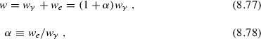
if we denote the transition probability by emitting photon by \(w_\gamma \), and the transition probability by the internal conversion process by \(w_e\). \(\alpha \) is called the internal conversion coefficient . If the transition energy is large to some extent, then \(\alpha \) is small, so that one can ignore the contribution of the internal conversion. On the other hand, the internal conversion becomes the main decay process if the excitation energy of the first excited \(2^+_1\) state is small as in the case of \({}^{238}_{~92}\)U, where it is about 45 keV. Equation (8.76) holds in this case as well. However, care should be taken when one tries to estimate the magnitude of \(\beta \) from the lifetime of the \(2^+_1\) state.
- 19.
Here, we add comments on the liquid-drop model. The experimental data show systematics given by

On the other hand, the liquid-drop model leads to

for vibrational excitations.
The prediction of the liquid-drop model Eq. (8.80) has a different mass number dependence from that of the experimental data given by Eq. (8.79). One reason of the discrepancy is the quantum mechanical effect, which plays important roles in nuclear physics. It is necessary to treat nucleus as a quantum liquid in order to handle nucleus in the liquid-drop model in a quantitatively proper way. For example, the classical liquid-drop model evaluates the potential energy by taking into account the effect of deformation only in the ordinary space in deriving the Hamiltonian for collective motions. Accurately, however, one needs to consider the effects of deformation in the momentum space as well as suggested by the uncertainty principle in quantum mechanics. This effect shows up, for example, in the vibrational excited states such as the giant quadrupole resonance (GQR) [39]. The discrepancy between the experimental data and the prediction of the liquid-drop model appears also regarding the moment of inertia of deformed nuclei.


References
H.J. Rose, G.A. Jones, Nature 307, 245 (1984)
B. Blank, M.J.G. Borge, Prog. Part. Nucl. Phys. 60, 403 (2008); B. Blank, M. Płoszajczak. Rep. Prog. Phys. 71, 046301 (2008)
K. Kato, K. Ikeda, Butsuri 61, 814 (2006); T. Myo, Y. Kikuchi, H. Masui, K. Kato. Prog. Part. Nucl. Phys. 79, 1 (2014)
D.M. Brink, N. Takigawa, Nucl. Phys. A 279, 159 (1977)
S.Y. Lee, N. Takigawa, Nucl. Phys. A 308, 189 (1978)
S.Y. Lee, N. Takigawa, C. Marty, Nucl. Phys. A 308, 161 (1978)
M. Abramowitz, I.A. Stegun, Handbook of Mathematical Functions with Formulas, Graphs, and Mathematical Tables (Dover, London, 1978)
M. Nogami, Nuclear Physics (Shoukabou, Tokyo, 1973). Japanese edn.
D.F. Jackson, M. Rhoades-Brown, Ann. Phys. (NY) 105, 151 (1977); S. A. Gurvitz, G. Kalbermann, Phys. Rev. Lett. 59, 262 (1987); S. A. Gurvitz. Phys. Rev. A 38, 1747 (1988)
S. Åberg, P.B. Semmes, W. Nazarewicz, Phys. Rev. C 56, 1762 (1997)
J.M. Blatt, V.F. Weiskopf, Theoretical Nuclear Physics (Wiley, New York, 1952)
M.A. Preston, Physics of the Nucleus (Addison-Wesley, London, 1962)
K. Kikuchi, M. Kawai, Nuclear Matter and Nuclear Reactions (North-Holland, Amsterdam, 1968)
S. Yoshida, M. Kawai, Nuclear Reactions (Asakura, Tokyo, 2002). Japanese edn.
A.M. Lane, R.G. Thomas, Rev. Mod. Phys. 30, 257 (1958)
E.P. Wigner, Phys. Rev. 70, 606 (1946); E.P. Wigner, L. Eisenbud. Phys. Rev. 72, 29 (1947)
T. Teichman, E.P. Wigner, Phys. Rev. 87, 123 (1952)
A. Arima, H. Horiuchi, K. Kubodera, N. Takigawa, Adv. Nucl. Phys. 5, 345 (1972)
B. Buck, A.C. Merchant, S.M. Perez, Phys. Rev. C 45, 2247 (1992); B. Buck, J. C. Johnson, A. C. Merchant, S. M. Perez. Phys. Rev. C 53, 2841 (1996)
I. Tonozuka, A. Arima, Nucl. Phys. A 323, 45 (1979)
C.M. Lederer, V. Shirley, Table of Isotopes, 7th edn. (Wiley, New York, 1978)
P. Hänggi, P. Talkner, M. Borkovec, Rev. Mod. Phys. 62, 251 (1990). and references therein
U. Weiss, Quantum Dissipative Systems (World Scientific, Singapore, 1999)
P. L. Kapur, R. Peierls, Proc. Roy. Soc. London A 163, 606 (1937); A. Schmid, Ann. Phys. (NY) 170, 333 (1986)
T. Kindo, A. Iwamoto, Phys. Lett. B 225, 203 (1989)
N. Takigawa, K. Hagino, M. Abe, Phys. Rev. C 51, 187 (1995)
N. Bohr, J.A. Wheeler, Phys. Rev. 56, 426 (1939)
H.A. Kramers, Physica 7(284), 284 (1940)
R. Kubo, M. Toda, N. Hashitsume, Statistical Physics II, Non-equilibrium Statistical Mechanics (Springer, New York, 1985)
H. Risken, The Fokker-Planck Equation (Springer, Berlin, 1989)
J.S. Langer, Ann. Phys. (NY) 41, 374 (1967); I. K. Affleck. Phys. Rev. Lett. 46, 388 (1981)
R.P. Feynman, A.R. Hibbs, Quantum Mechanics and Path Integrals (McGraw-Hill, New York, 1965)
H. Grabert, P. Olschowski, U. Weiss, Phys. Rev. B 36, 1931 (1987)
N. Takigawa, M. Abe, Phys. Rev. C 41, 2451 (1990)
Y. Abe, C. Gregoire, H. Delagrange, J. Phys. 47, C4 (1986); T. Wada, Y. Abe, N. Carjan, Phys. Rev. Lett. 70, 3538 (1993); Y. Abe, S. Ayik, P.-G. Reinhard, E. Suraud, Phys. Rep. 275, 49 (1996)
P. Fröbrich, R. Lipperheide, Theory of Nuclear Reactions (Clarendon Press, Oxford, 1996)
Aage Bohr, Ben R. Mottelson, Nuclear Structure, vol. I (Benjamin, New York, 1969)
S. Raman, C.W. Nestor Jr., P. Tikkanen, At. Data Nucl. Data Tables 78(1), 1 (2001)
P. Ring, P. Schuck, The Nuclear Many-Body problem (Springer, Berlin, 1980)
A.B. Balantekin, N. Takigawa, Rev. Mod. Phys. 70, 77 (1998)
M. Dasgupta, D.J. Hinde, N. Rowley, A.M. Stefanini, Ann. Rev. Nucl. Part. Sci. 48, 401 (1998)
K. Hagino, N. Rowley, A.T. Kruppa, Comp. Phys. Commun. 123, 143 (1999)
H. Esbensen, Nucl. Phys. A 352, 147 (1981)
K. Hagino, N. Takigawa, Butsuri 57, 588 (2002)
K. Hagino, N. Takigawa, Prog. Theor. Phys. 128, 1001 (2012)
K. Yagi, Nuclear Physics (Asakura, Tokyo, 1971). Japanese edn.
Author information
Authors and Affiliations
Corresponding author
Rights and permissions
Copyright information
© 2017 Springer Japan
About this chapter
Cite this chapter
Takigawa, N., Washiyama, K. (2017). Nuclear Decay and Radioactivity. In: Fundamentals of Nuclear Physics. Springer, Tokyo. https://doi.org/10.1007/978-4-431-55378-6_8
Download citation
DOI: https://doi.org/10.1007/978-4-431-55378-6_8
Published:
Publisher Name: Springer, Tokyo
Print ISBN: 978-4-431-55377-9
Online ISBN: 978-4-431-55378-6
eBook Packages: Physics and AstronomyPhysics and Astronomy (R0)