
Abstract
Jan Tinbergen’s, “The Appraisal of Road Construction: Two Calculation Schemes [18],” that appeared in RE & Stat. on August 1957, which gave us a great profound impression, coincided with the mentality of the times when we are about to study on the real economic research of expressways, right on the heels of Report on Kobe–Nagoya Expressway Survey (for the Ministry of Construction, Government of Japan, August 8, 1956, 188 pp.) by a group of experts headed by Ralph J. Watkins. (10 months later, the introductory paper of [18] by Yukihide Okano came out in the periodical: Expressways, Express Highway Research Foundation of Japan.)
Access this chapter
Tax calculation will be finalised at checkout
Purchases are for personal use only
Notes
- 1.
The terms “goods ” and “commodities” are used to include “services.”
- 2.$$ {\sum}_{i=2}^4{Q}_{1i}\equiv 1 $$(9.50′)
- 3.
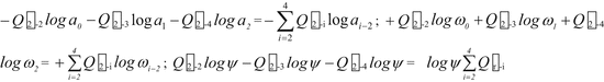
- 4.$$ {Q}_{12} \log {a}_0-{Q}_{13} \log {a}_1-{Q}_{14} \log {a}_2={\displaystyle \sum_{i=2}^4{Q}_{1i} \log {a}_{i-2}};\;{Q}_{12} \log {\omega}_0+{Q}_{13} \log {\omega}_1+{Q}_{14} \log {\omega}_2={\displaystyle \sum_{i=2}^4{Q}_{1i}{\omega}_{i-2}};{Q}_{12} \log \psi -{Q}_{13} \log \psi -{Q}_{14} \log \psi ={\displaystyle \sum_{i=2}^4{Q}_{1i} \log \psi } $$
- 5.
- 6.
- 7.
- 8.
[ ]* and ( )* are not a matrix but a column vector.
- 9.
The 1 × log p r of the 4th term in the right-hand side of (9.a4) removed to the 2nd term of the left hand side of (9.a6). The 2nd term of (9.a5) will be entered into the central term of eq. (9.68). Remained term appears in the 4th term of (9.a6). Namely, by the [1 − B11 r] of (9.a5), the 4th term of (9.a4) is divided into two parts.
- 10.
\( {B}_{i1}^r \log {k}_r-{\displaystyle \sum_{s=2}^{M+2}{B}_{is}^r \log {\alpha}_{s-2,r}} \) = Eq. (9.67).
- 11.
Due to E 11 = 0, the 1st term is zero.
- 12.
Eq. (9.73) \( \to {\beta}_r^y\cdot {\alpha}_{ir}\Leftarrow {\beta}_{ir}^x \) → To substitute.
- 13.
Due to assumption (iii) of 9.1.3., that is, E 22 = 0, the 1st term is zero.
- 14.
The 1st term is zero, due to E 33 .
- 15.
i ≠ j: The meaning is that D ii is excluded.
- 16.
−μ j + μ j = 0.
- 17.
B ii = 0 (by definition).
- 18.
The identity (9.53) of 9.1.8. can be applied.
- 19.
A 11 B 1j = ((c)); A 12 B 2j → ((e)).
- 20.
(9.52) can be applied.
- 21.
The A ii only remains, others are to be zero.
- 22.
E 01 = 1, from (ii) (3) of 9.1.3.
- 23.
E 1 − 2, 1 B 11 = E i − 2, 1 B j1 of (5) above is substituted.
- 24.
Here, the 1st term in the left hand side of eq. (5) is substituted for every term of eq. (3)′ corresponding to respective subscripts (i = 2 … M + 2).
- 25.
Definition (9.75) is substituted for the denominator.
- 26.
Here, subscript 1 shows to be transport service industry and subscript M to be resource industry , respectively.
- 27.
Repeatedly, the direct benefits in generation base are different from the intention of transport researchers in the early stage and are vague depending on the way of assumption of the partial equilibrium.
- 28.

References
Kohno, Hirotada. 1976. Formation process of the indirect economic effects. Expressways and Automobiles XIX(4): 21–29.
Kohno, H. 1979. Valuation of social benefits. In Modern auto transportation treatise, ed. Genpachiro Konno and Yukihide Okano, 108–132. Tokyo: The University of Tokyo Press.
Kohno, Hirotada. 1983. Regional development effects brought about by the public investments. Studies in regional science, Vol. 13, The 19th JSRSA annual meeting report of 1982, Japan section of RSA, Dec. (S.58), pp. 57–81.
Kohno, H. 1987. Social benefits of transport investment—Theoretical synthesis. In OECD highway committee: Expert meeting and symposium in the appraisal of social and economic effects of road network improvement, pp. 80–92, Yokohama, May 26–28th.
Kohno, H. 2007. Simultaneous equilibrium of industries and enterprises in the long range—In the case where there is the Marshallian external economies. In The principle of economics I∙II: Micro economics∙macro economics, pp. 116–121, Socio Economic Planning Office, April 9th.
Kohno, H., and Y. Higano. 1981. Comprehensive valuation (p. 274). In The regional science in Japan: Survey II, studies in regional science, Vol. II, pp. 221–330, JRSA.
Kohno, Hirotada, and Yoshiro, Higano. 1982. Synthesis of Tinbergen and Mohring’s propositions on the indirect benefits of public investment. A paper presented to the 29th North American meetings, Pittsburgh, November 12–14.
Kohno, Hirotada, and Yoshiro, Higano. 1993. A proof of the existence of Tinbergen multiplier on the indirect benefits of public investment. A paper prepared for the 40th North American meetings of the RSAI, Houston, November 11–14.
Hicks, John Richard. 1939. Value and capital. Oxford: The Clarendon Press in the University of Oxford.
Hicks, J.R. 1951. Supplement to the chap.2 consumer surplus. In Value and capital (Translated by Takuma Yasui, Hisao Kumagai, Iwanamigendai Sosho, pp. 53–59).
Julius, Margolis. 1957. Secondary benefits, external economies, and the justification of public investment. The Review of Economics and Statistics XXXIX(3): 284–291. (Translated by Katsuyuki Kurashimo. 1962. Expressways and Automobiles 5 (12): 52–59).
Meade, J.E. 1952. External economies and diseconomies in a competitive situation. Economic Journal LXII(245): 54–67.
Mohring, Herbert, and Mitchell Harwitz. 1962. Highway benefits—An analytical framework. Evanston: The Transportation Center at Northwestern University by Northwestern University Press.
Nikaido, Fukukane. 1960. Mathematical method of modern economics—Introductory analyses by topological mathematics. Tokyo: Iwanami-shoten.
The Nikkei. 2015. Traffic volumes of circular highways of central Tokyo such as Loop 7, etc. are cutted down of 5 percent; and, Congestion loss time of 40 percent owing to the completion of circumferential expressway. p. 35, April 25th.
Samuelson, Paul A. 1966. Constancy of the marginal utility of income. In The collected scientific papers of Paul A. Samuelson, vol. 1, ed. Joseph E. Stiglitz, 37–53. Cambridge, MA: MIT Press.
Scitovsky, Tibor. 1954. Two concepts of external economies. Journal of Political Economy LXII(2): 143–151.
Tinbergen, Jan. 1957. The appraisal of road construction: Two calculation schemes. The Review of Economics and Statistics XXXIX(3): 241–249. (Translated by Yukihide Okano. 1958. Expressways 1(2): 37–47 & 50.).
Yasui, Takuma, and Fukuoka, Masao. 1984. Special talk: L. Walras and the modern economics (modern economics series No.69). Weekly Toyo Keizai a special issue, April 20th, pp. 54–66.
Yasui, Takuma, and Fukuoka, Masao. 1984. Special talk continued: the 150th memory of L. Walras birth and the modern economics (modern economics series No. 70). Weekly Toyo Keizai a special issue, September. 27th, pp. 100–108.
Kanemoto, Y., and K. Mera. 1985. General equilibrium analysis of the benefits of large transportation improvement. Regional Science and Economics 15: 343–363.
Author information
Authors and Affiliations
Appendix
Appendix
9.1.1 Result of Simulation
Simulation results of the models I, II, and III are as follows:
[Model I (M = 4)]
Below, models II and III:
[Model II (M = 5)]
[Model III (M = 6)]
Note that, in all the models, \( \widehat{\Omega} \) and \( \tilde{\Omega} \) are dominant diagonal matrixes which have negative diagonal elements, which imply that the equilibrium of the market is locally stable about both \( \widehat{P} \) and \( \tilde{P} \).
Rights and permissions
Copyright information
© 2016 Springer Japan
About this chapter
Cite this chapter
Kohno, H. (2016). Verification of Independent Existence Theory Depended on the Market Equilibrium Model: Based on the Great Discrepancy of the Benefits in Generation Base vs. the Benefits in Incidence Base. In: Economic Effects of Public Investment. New Frontiers in Regional Science: Asian Perspectives, vol 1. Springer, Tokyo. https://doi.org/10.1007/978-4-431-55224-6_9
Download citation
DOI: https://doi.org/10.1007/978-4-431-55224-6_9
Published:
Publisher Name: Springer, Tokyo
Print ISBN: 978-4-431-55223-9
Online ISBN: 978-4-431-55224-6
eBook Packages: Economics and FinanceEconomics and Finance (R0)