Control System Basics and PID Control

Abstract

The first automatic control system is said to be the governor (a speed regulator) for the steam engine, invented by James Watt. The speed regulator enabled the steam engine to be used as a practical power source, starting the industrial revolution. “Control” is defined as “adding required operation to an object so that it can be adapted for a certain purpose” (JIS automatic control terms). Control can be divided into two main categories: automatic and manual. Automatic control is divided into feedback control, feed-forward control, sequential control, and others. Automatic control can be implemented by control systems among which single-variable control systems (single-input, single-output systems) are one type.

An erratum to this chapter can be found at http://dx.doi.org/10.1007/978-4-431-54195-0_12

Appendices

Laplace Transform Formulae

1.1 Definitions of Laplace transform

We denote the output as y(t) when the input x(t) is added to a system.

A transfer function connects the input and output by

$$ (\mathrm{ Laplace}\ \mathrm{ transform}\ \mathrm{ of}\ \mathrm{ output})=(\mathrm{ transfer}\ \mathrm{ function})\times (\mathrm{ Laplace}\ \mathrm{ transform}\ \mathrm{ of}\ \mathrm{ input}) $$

which is based mathematically on the Laplace transform.

The Laplace transform is an integral transform that maps the time function f(t) defined by t ≥ 0 to the complex function F(s) using the integral kernel e^−st (s is a complex number, and called a Laplace operator). The following defines the Laplace transform. Usually, f(t) = 0 if t < 0.

$$ F(s)=\int_0^{\infty } {f(t){{\mathrm{ e}}^{-st }}\mathrm{ d}t} $$

As the integral range of this expression reaches [0, ∞), it is a concern whether the integral is convergent. We may regard it as convergent for time functions commonly encountered in control engineering.

Next, the operation that obtains the time function f(t) corresponding to the given Laplace transform F(s) is called the inverse Laplace transform, and it is expressed below.

$$ f(t)=\frac{1}{{2\pi j}}\int_{c-j\infty}^{c+j\infty } {{F}(s){{{e}}^{st }}\mathrm{ d}s} $$

1.2 Laplace Transform Formulae

1.2.1 Laplace Transform Formula for Time Derivative

$$ \begin{array}{llll} \int_0^{\infty } {f^{\prime}(t){e^{-st}}\mathrm{ d}t} =sF(s)-f(0) \hfill \\ \int_0^{\infty } {{f^{(n)}}(t){{\mathrm{ e}}^{-st }}\mathrm{ d}t={s^n}F(s)-{s^{n-1}}f(0)-{s^{n-2 }}{f}^{\prime}(0)-\cdots -{f^{(n-1) }}(0)}\hfill \end {array} $$

where f(0), f ^(k)(0) denote the initial values of the kth order derivative. When every initial value is zero, the nth order derivative in a time domain is dealt with by multiplying F(s) by s ⁿ in the s domain.

1.2.2 Laplace Transform Formula for Time Integration

The Laplace transform formula for time integration are given by the following expression.

$$ \begin{array}{llll}\int_0^{\infty } {\left( {\int_0^t {f(\tau)\mathrm{ d}\tau } } \right)}{{\mathrm{ e}}^{-st }}\mathrm{d}t=\frac{1}{s}F(s) \hfill \\ \int_0^{\infty } {\left( {\int_0^t{\left( {\int_0^{{{t_{n-1}}}} \cdots \left( {\int_0^{{{t_2}}}{\left( {\int_0^{{{t_1}}} {f(\tau )\mathrm{ d}\tau } }\right)\mathrm{ d}{t_1}} } \right)\mathrm{ d}{t_2}\cdots } \right)}\mathrm{ d}{t_{n-1 }}} \right)}{{\mathrm{ e}}^{-st }}\mathrm{d}t=\frac{1}{{{s^n}}}F(s) \hfill \end{array} $$

An nth multiple integral in a time domain is dealt with by dividing F(s) by s ⁿ in the s domain.

1.2.3 Time Transition Formula

The time transition formula is as follows.

$$ \int_0^{\infty } {f(t-a){{\mathrm{ e}}^{-st }}\mathrm{ d}t} ={{\mathrm{ e}}^{-as }}F(s),\quad a>0 $$

1.2.4 Convolution Integral in a Time Domain

The convolution integral in a time domain is as follows.

$$ \int_0^{\infty } {\left( {\int_0^t {{f_1}(\tau ){f_2}(t-\tau )\mathrm{ d}\tau } } \right)}{{\mathrm{ e}}^{-st }}\mathrm{ d}t={F_1}(s){F_2}(s) $$

1.2.5 Functions Familiar to Control Engineering

The following functions are commonly used in control engineering (hereafter, the Laplace transform is expressed by the symbol $L$ ).

$$ (1)\quad L(au(t))=\frac{a}{s},\quad u(t):\quad \mathrm{ Step}\;\mathrm{ function} $$

$$ (2)\quad L(a\delta (t))=a,\quad \delta (t):\quad \mathrm{ Impulse}\;\mathrm{ function} $$

$$ (3)\quad L({{\mathrm{ e}}^{at }})=\frac{1}{s-a } $$

$$ (4)\quad L\left( {\frac{1}{a}{{\mathrm{ e}}^{{-\frac{t}{a}}}}} \right)=\frac{1}{1+as } $$

$$ (5)\quad L(t)=\frac{1}{{{s^2}}} $$

$$ (6)\quad L\left( {\frac{1}{(n-1)! }{t^{n-1 }}} \right)=\frac{1}{{{s^n}}} $$

$$ (7)\quad L\left( {{{\mathrm{ e}}^{{-\delta t}}}\sin (\omega t\pm \phi )} \right)=\frac{{\omega\cos\phi \pm (s+\delta )\sin\phi }}{{{{{(s+\delta )}}^2}+{\omega^2}}} $$

$$ (8)\quad L\left( {{{\mathrm{ e}}^{{-\delta t}}}\cos (\omega t\pm \phi )} \right)=\frac{{(s+\delta )\cos\phi \mp \omega\sin\phi }}{{{{{(s+\delta )}}^2}+{\omega^2}}} $$

1.2.6 Expansion Theorem of Heviside

The Laplace transform F(s) is assumed to be given by the following rational function.

$$F(s) = \frac{N{s}}{D(s)} = \frac{b_{m}s^{m} + b_{m-1}s^{m-1} + \cdots + b_{1}s + b_{0}}{s^{n} + a_{n-1}s^{n-1} + \cdots + a_{1}s + a_{0}}, \quad (n > m)$$

Then the inverse transform f(t) can be obtained in the following expression:

$$ f(t)={k_1}{{\mathrm{ e}}^{{{p_1}t}}}+{k_2}{{\mathrm{ e}}^{{{p_2}t}}}+\cdots +{k_n}{{\mathrm{ e}}^{{{p_n}t}}} $$

where

p ₁, p ₂, …, p _n : The root of the denominator polynomial D(s) (no repeated root is assumed)

${k_i}=\frac{{N({p_i})}}{{D^{\prime}({p_i})}},\quad i=1,2,\ldots,n,{D}^{\prime}(s)$ is the derived function of D(s).

1.2.7 Final-Value Theorem and Initial-Value Theorem

When sF(s) is nonsingular on the right-hand side of the s plane, including the imaginary axis, the following theorems may be applied.

Final-value theorem: $\mathop{\lim}\limits_{{t\to \infty }}f(t)=\mathop{\lim}\limits_{{s\to 0}}s\cdot F(s)$

Initial-value theorem: $\mathop{\lim}\limits_{{t\to 0+}}f(t)=\mathop{\lim}\limits_{{s\to \infty }}s\cdot F(s)$

Pade Approximation

2.1 Pade Approximation Method

It is assumed that G(s) is a given transfer function. We consider a problem to approximate it by a rational function with a polynomial of the nth degree of s as denominator, and a polynomial of the mth degree as numerator. This is called the (n, m) type Pade approximation, which can be obtained by the following procedure.

Step <1>

Expand the given G(s) by Maclaurin’s theorem.

The expression is

$$ G(s)={g_0}+{g_1}s+{g_2}{s^2}+\cdots +{g_k}{s^k}+\cdots +{g_{m+n }}{s^{m+n }}+\cdots $$

(5.40)

where

$$ {g_k}={{\left[ {\frac{1}{k!}\cdot \frac{{{{\mathrm{ d}}^k}}}{{\mathrm{ d}{s^k}}}G(s)} \right]}_{s=0 }},\quad k=0,1,2,3,\ldots, $$

(5.41)

Step <2>

Give the rational function H(s) that approximates G(s) by the following expression:

Usually H(s) is assumed to be a proper rational function and m ≦ n.

$$ H(s)=\frac{{{b_0}+{b_1}s+\cdots +{b_m}{s^m}}}{{1+{a_1}s+\cdots +{a_n}{s^n}}}={h_0}+{h_1}s+\cdots +{h_{m+n }}{s^{m+n }}+\cdots $$

(5.42)

Here, the last expression is a polynomial resulted by performing division calculation of the numerator by the denominator of the rational function.

Step <3>

Find (m + n + 1) numbers of unknown coefficients (a ₁, a ₂, …, a _n , and b ₀, b ₁, b ₂, …, b _m ) of the expression (5.42) so that the initial (m + n + 1) terms of the expressions (5.40) and (5.42) match each other.

Actually, unknown coefficients a _i and b _j can be obtained by using the following steps. First, the following equation is obtained from Step <3>:

$$ ({g_0}+{g_1}s+\cdots +{g_k}{s^k}+\cdots )(1+{a_1}s+\cdots +{a_n}{s^n})={b_0}+{b_1}s+\cdots +{b_m}{s^m} $$

The left side is expanded to yield the following expression:

$$ \sum\limits_{l=1}^{\infty } {\left( {\sum\limits_{k+i=l } {{g_k}{a_i}} } \right)} {s^l}-\sum\limits_{j=0}^m {{b_j}{s^j}} =-\sum\limits_{k=0}^{\infty } {{g_k}{s^k}} $$

(5.43)

where other than $n\ge i\ge 1$: ${a_i}=0$ other than $m\ge j\ge 1:{b_j}=0,k<0:{g_k}=0$

Assuming that coefficients from the 0th order term to the (n + m)th order term of s on both sides of Eq. (5.43) are equal, then we obtain the following (n + m + 1) equations.

0th order term: $-{b_0}=-{g_0}$

1st order term: $({g_0}{a_1})-{b_1}=-{g_1}$

2nd order term: $({g_1}{a_1}+{g_0}{a_2})-{b_2}=-{g_2}$

3rd order term: $({g_2}{a_1}+{g_1}{a_2}+{g_0}{a_3})-{b_3}=-{g_3}$

$\vdots$

mth order term: $({g_{m-1 }}{a_1}+{g_{m-2 }}{a_2}+\cdots +{g_{m-n }}{a_n})-{b_m}=-{g_m}$

(m + 1)th order term $({g_m}{a_1}+{g_{m-1 }}{a_2}+\cdots +{g_{m-(n-1) }}{a_n})+0=-{g_{m+1 }}$

·

·

(n + m)th order term $({g_{n+m-1 }}{a_1}+{g_{n+m-2 }}{a_2}+\cdots +{g_m}{a_n})+0=-{g_{m+n }}$

Those (n + m + 1) numbers of equations can be expressed as the following easily viewable equations by using a coefficient matrix, unknown variable vectors, and known vectors.

$$ \left[ {\begin{array}{*{20}{c}} 0 & 0 & 0 & \cdots & 0 & {-1} & \cdots & 0 \\ {{g_0}} & 0 & 0 & \cdots & 0 & 0 & \vdots & 0 \\ {{g_1}} & {{g_0}} & 0 & \cdots & 0 & 0 & \vdots & 0 \\ {{g_2}} & {{g_1}} & {{g_0}} & \cdots & 0 & 0 & \vdots & 0 \\ \vdots & \vdots & \vdots & \vdots & \vdots & 0 & \cdots & 0 \\ {{g_{m-1 }}} & {{g_{m-2 }}} & {{g_{m-3 }}} & \cdots & {{g_{m-n }}} & 0 & \cdots & {-1} \\ {{g_m}} & {{g_{m-1 }}} & {{g_{m-2 }}} & \cdots & {{g_{m-n+1 }}} & 0 & \cdots & 0 \\ \vdots & \vdots & \vdots & \cdots & \vdots & \vdots & \vdots & \vdots \\ {{g_{n+m-1 }}} & {{g_{n+m-2 }}} & {{g_{n+m-3 }}} & \cdots & {{g_m}} & 0 & \vdots & 0 \\ \end{array}} \right]\,\,\,\left[ {\begin{array}{*{20}{c}} {{a_1}} \\ {{a_2}} \\ {{a_3}} \\ \vdots \\ \vdots \\ {{a_n}} \\ {{b_0}} \\ {{b_1}} \\ \vdots \\ {{b_m}} \\ \end{array}} \right]=\left[ {\begin{array}{*{20}{c}} {-{g_0}} \\ {-{g_1}} \\ {-{g_2}} \\ \vdots \\ {-{g_m}} \\ {-{g_{m+1 }}} \\ {-{g_{m+2 }}} \\ \vdots \\ {-{g_{m+n }}} \\ \end{array}} \right] $$

This matrix and vector representation enables us to obtain values a ₁, a ₂, …, a _n from the following expression.

$$ \left[ {\begin{array}{cccccccccc} {{g_m}} & {{g_{m-1 }}} & {{g_{m-2}}} & \cdots & {{g_{m-n+1 }}} \\{{g_{m+1 }}} & {{g_m}} & {{g_{m-1}}} & \cdots & {{g_{m-n+2 }}} \\ \vdots & \vdots & \vdots & \cdots & \vdots \\{{g_{n+m-1 }}} & {{g_{n+m-2 }}} & {{g_{n+m-3 }}} & \cdots & {{g_m}} \\\end{array}} \right]\left[ {\begin{array}{cccccccccc} {{a_1}} \\{{a_2}} \\{{a_3}} \\\vdots \\{{a_n}} \\\end{array}} \right]=\left[{\begin{array}{ccccccccc} {-{g_{m+1 }}} \\{-{g_{m+2 }}} \\\vdots \\{-{g_{m+n}}} \\\end{array}} \right] $$

It is

$$ \left[ {\begin{array}{cccccccc} {{a_1}} \\{{a_2}} \\{{a_3}} \\\vdots \\{{a_n}} \\\end{array}} \right]=\left[ {\begin{array}{cccccccccc}{{g_m}} & {{g_{m-1 }}} & {{g_{m-2 }}} & \cdots & {{g_{m-n+1 }}} \\{{g_{m+1 }}} & {{g_m}} & {{g_{m-1 }}} & \cdots & {{g_{m-n+2 }}} \\\vdots & \vdots & \vdots & \cdots & \vdots \\{{g_{n+m-1 }}} & {{g_{n+m-2 }}} & {{g_{n+m-3 }}} & \cdots & {{g_m}} \\\end{array}} \right]{^{-1 }} \cdot \left[ {\begin{array}{ccccccccc} {-{g_{m+1 }}} \\{-{g_{m+2 }}} \\\vdots \\{-{g_{m+n }}} \\\end{array}} \right] $$

(5.44)

Similarly, b ₀, b ₁, b ₂, …, b _m can be obtained from the following expression:

$$ \left[ {\begin{array}{cccccccc} {{b_1}} \\{{b_2}} \\{{b_3}} \\\vdots \\{{b_m}} \\\end{array}} \right]=\left[ {\begin{array}{cccccccc} 0 & 0 & 0 & \cdots & 0 \\{{g_0}} & 0 & 0 & \cdots & 0 \\{{g_1}} & {{g_0}} & 0 & \cdots & 0 \\\vdots & \vdots & \vdots & \cdots & \vdots \\{{g_{m-1 }}} & {{g_{m-2 }}} & {{g_{m-3 }}} & {} & {{g_{m-n}}} \\\end{array}} \right]\cdot \left[ {\begin{array}{cccccccc} {{a_1}} \\{{a_2}} \\{{a_3}} \\\vdots \\{{a_n}} \\\end{array}} \right]+\left[{\begin{array}{ccccccccc} {{g_0}} \\{{g_1}} \\{{g_2}} \\\vdots \\{{g_m}} \\\end{array}} \right] $$

(5.45)

2.2 Pade Approximation in a Dead Time System

We obtain the (2, 2) type Pade approximation of the transfer function G(s) = e^−Ls in a dead time system. First, according to Step <1> above, to expand from the first to 4th order terms, Maclaurin’s theorem is used.

$$ {{\mathrm{ e}}^{-Ls }}\cong 1+(-L)s+\left( {\frac{{{L^2}}}{2}} \right){s^2}+\left( {-\frac{{{L^3}}}{6}} \right){s^3}+\left( {\frac{{{L^4}}}{24 }} \right){s^4}+\cdots $$

(5.46)

Therefore, we obtain the next expression.

$$ {g_0}=1,\quad {g_1}=-L,\quad {g_2}=\frac{{{L^2}}}{2},\quad {g_3}=-\frac{{{L^3}}}{6},\quad {g_4}=\frac{{{L^4}}}{24 },\ldots,{g_k}=\frac{{{(-L)^k}}}{k! },\ldots $$

Substituting these into the expression (5.44) yields

$$ \left| {\left. {\begin{array}{llll} {{a_1}} \\{{a_2}} \\ \end{array}} \right]} \right.={{\left[ {\begin{array}{lllll}{\frac{{{L^2}}}{2}} & {-L} \\{-\frac{{{L^3}}}{6}} & {\frac{{{L^2}}}{2}} \\ \end{array}} \right]}^{-1 }}\cdot \left[ {\begin{array}{llll} { \frac{{{L^3}}}{6}}\\{-\frac{{{L^4}}}{24}} \\ \end{array}} \right] $$

$$ {a_1}=-\frac{L}{2},\quad \quad {a_2}=\frac{{{L^2}}}{12 } $$

Also by using the expression (5.44), we obtain ${b_0}=1,\quad \quad {b_1}=-\frac{L}{2},\quad \quad {b_2}=\frac{{{L^2}}}{12 }$.

Consequently, the (2, 2) type Pade approximation in a dead time system is:

$$ G(s)={{\mathrm{ e}}^{-Ls }}\cong \frac{{1-\frac{1}{2}Ls+\frac{1}{12 }{(Ls)^2}}}{{1+\frac{1}{2}Ls+\frac{1}{12 }{(Ls)^2}}} $$

(5.47)

Chapter 5 Exercises

• 1. Obtain Laplace transforms of the following functions

  <1> sin ωt, where ω is positive.

  <2> con ωt, where ω is positive.

  <3> f(at) where a is positive.

• 2. The impulse input x(t) = δ(t) has been given to a system with the initial value 0 for all the state variables. Then the response is measured as follows:

  $$ y(t)=\left\{ \begin{array}{llllllllll} 0 & : {t<0} \\ \frac{a}{T}t & : {0\le}t{\le T}. \\ 0 & : {T<{t}} \end{array} \right. $$

  Obtain the system transfer function from this input port to the output.

• 3. Obtain the Laplace transform of the following function

  $$ f(t)=\left\{ {\begin{array}{lllllllllll} 0 & : \hfill & {t<0} \hfill \\a\sin \left( {\frac{{2\pi }}{T}t} \right)& : \hfill & {0\le t\le \frac{T}{2}} \hfill \\ 0 & : \hfill & \frac{T}{2}<{t} \hfill \end{array}} \right. $$

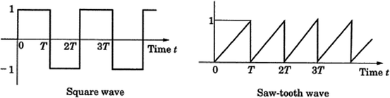
• 4. Obtain the Laplace transforms of a square wave and a saw-tooth wave which are shown in the following figures.

  <1> Square waveform (with amplitude 1, and cycle 2T)

  <2> Saw-tooth waveform (with unilateral amplitude 1, and cycle T)

  

• 5. Obtain the inverse Laplace transform of the following expression.

  $$ F(s)=\frac{k}{as(1+Ts) } $$

  (Clue) Use the expansion theorem ${L^{-1 }}\left[ {\frac{P(s) }{sQ(s) }} \right]=\frac{P(0) }{Q(0) }+\sum\limits_{h=2}^n {\frac{{P({s_h})}}{{{s_h}{Q}^{\prime}({s_h})}}} {{\mathrm{ e}}^{{{s_h}t}}}$.

  Assume that Q(s) = 0 has n − 1 pieces of simple root.

• 6. Derive the transfer function of the expression (5.6).

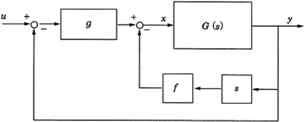
• 7. Consider a system expressed by the following motion equation.

  $$ m\frac{{{{\mathrm{ d}}^2}y}}{{\mathrm{ d}{t^2}}}+c\frac{{\mathrm{ d}y}}{{\mathrm{ d}t}}=kx $$

  where x is an input variable, y is an output variable, and m, c, and k are constants of the system.

  (1) Obtain the transfer function G(s) of this system.

  (2) Suppose that feedback control is incorporated in the system as shown in the figure. Obtain the closed-loop transfer function from the input u to output y (the 39th examination for chief engineer of reactors in Japan)

  

• 8. Prove that the block diagram shown in Fig. 5.16 is equivalent to that of a PID controller. Also confirm that the mutual interference coefficient is (1 + T ₂/T ₁).

• 9. In the design example in Sect. 5.6, we neglected the steam manipulated variable z(t) because it is negligibly small compared with the steady-state flow rate m(=2.3 kg/m), and obtained the expressions (5.34) and (5.35). Obtain the transfer function when the steam flow rate z(t) is not neglected.

• 10. It is natural that the (2, 2) type approximation (5.47) indicates a different response from that of the dead time system e^−Ls. However, to approximate the transfer function of (a dead time system) + (a high order system) by the rational function of s, a Pade approximation is effective. Discuss the reasons.

• 11. Obtain the Pade approximation of $\frac{5}{{{s^2}+2.5s+5}}{{\mathrm{ e}}^{-Lt }}$, a coupled system of dead time system + 2nd order oscillation system.

Bibliography

Bennett S (1998) History of control engineering 1800–1930, and history of control engineering 1930–1955. Corona Sha, Tokyo (in Japanese)
Kondo B, Fujii K (1972) Control engineering for college course. Ohm Sha, Tokyo (in Japanese)
Izawa K (1954) Introduction to automatic control. Ohm Sha, Tokyo (in Japanese)
Suda N et al (1992) PID control. Asakura Publishing, Tokyo (in Japanese)
Furuta K, Tomita T (1990) Report of current advanced control technology. J Soc Instrum Control Eng 29(10):77–82 (in Japanese)
The MathWork MATLAB Ver.5.2, User’s Guide (1998)
Author information
Authors and Affiliations
Editor information
Editors and Affiliations