Algebraic Semantics for Nelson’s Logic $\mathcal {S}$

Abstract

Besides the better-known Nelson’s Logic and Paraconsistent Nelson’s Logic, in “Negation and separation of concepts in constructive systems” (1959), David Nelson introduced a logic called $\mathcal {S}$ with the aim of analyzing the constructive content of provable negation statements in mathematics. Motivated by results from Kleene, in “On the Interpretation of Intuitionistic Number Theory” (1945), Nelson investigated a more symmetric recursive definition of truth, according to which a formula could be either primitively verified or refuted. The logic $\mathcal {S}$ was defined by means of a calculus lacking the contraction rule and having infinitely many schematic rules, and no semantics was provided. This system received little attention from researchers; it even remained unnoticed that on its original presentation it was inconsistent. Fortunately, the inconsistency was caused by typos and by a rule whose hypothesis and conclusion were swapped. We investigate a corrected version of the logic $\mathcal {S}$, and focus on its propositional fragment, showing that it is algebraizable in the sense of Blok and Pigozzi (in fact, implicative) with respect to a certain class of involutive residuated lattices. We thus introduce the first (algebraic) semantics for $\mathcal {S}$ as well as a finite Hilbert-style calculus equivalent to Nelson’s presentation; we also compare $\mathcal {S}$ with the other two above-mentioned logics of the Nelson family. Our approach is along the same lines of (and partly relies on) previous algebraic work on Nelson’s logics due to M. Busaniche, R. Cignoli, S. Odintsov, M. Spinks and R. Veroff.

Appendix: Proofs of the Some of the Main Results

Theorem 1

The calculus $\vdash _{{\mathcal {S}}}$ is implicative, and thus algebraizable.

Proof

In the case of ${\mathcal {S}}$, the term $\alpha ({\varphi }, \psi )$ may be chosen to be ${\varphi }\Rightarrow \psi$. We will make below free use of Proposition 2.

IL1 follows immediately from axiom (A1), while IL2 follows from rule $\mathrm {\texttt {(E)}}$. IL3 follows from (MP) and IL4 follows from $\mathrm {(\Rightarrow \texttt {r})}$. We are left with proving that $\Rightarrow$ respects IL5 for each connective $\bullet \in \{ \wedge , \vee , \Rightarrow , {\sim }\}$.  

$({\sim })$ :

$\{({\varphi }\Leftrightarrow \psi ), (\psi \Leftrightarrow {\varphi }) \} \vdash _{{\mathcal {S}}} {\sim }{\varphi }\Leftrightarrow {\sim }\psi$ holds by axiom (A5) and the (derived) rule (MP).

$(\wedge )$ :

We must prove that $\{ ({\varphi }_{1} \Leftrightarrow \psi _{1}), ({\varphi }_{2} \Leftrightarrow \psi _{2})\} \vdash _{{\mathcal {S}}} ({\varphi }_{1}\wedge {\varphi }_{2}) \Leftrightarrow (\psi _{1} \wedge \psi _{2})$. From Proposition 1(1–2) we have $\vdash _{{\mathcal {S}}} ({\varphi }_{1} \wedge {\varphi }_{2}) \Rightarrow {\varphi }_{1}$ and $\vdash _{{\mathcal {S}}} ({\varphi }_{1} \wedge {\varphi }_{2}) \Rightarrow {\varphi }_{2}$. Then:

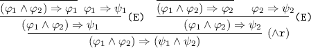
The remainder of the proof is analogous.

$(\vee )$ :

We must prove that $\{ ({\varphi }_{1} \Leftrightarrow \psi _{1}), ({\varphi }_{2} \Leftrightarrow \psi _{2})\} \vdash _{{\mathcal {S}}} ({\varphi }_{1}\vee {\varphi }_{2}) \Leftrightarrow (\psi _{1} \vee \psi _{2})$. From Proposition 1(3–4), $\psi _{1} \Rightarrow (\psi _{1} \vee \psi _{2})$ and $\psi _{2} \Rightarrow (\psi _{1} \vee \psi _{2})$ are derivable. Then:

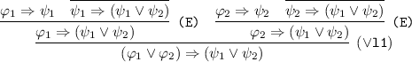
The remainder of the proof is analogous.

$(\Rightarrow )$ :

We must prove that $\{ (\theta \Leftrightarrow {\varphi }), (\psi \Leftrightarrow \gamma ) \}\vdash _{{\mathcal {S}}} (\theta \Rightarrow \psi ) \Leftrightarrow ({\varphi }\Rightarrow \gamma )$. This time, we have:

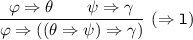
Taking $\psi$ as $\theta \Rightarrow \psi$ in Proposition 1(5), we have:

The remainder of the proof is analogous.

 

Proposition 3

Let $\mathbf {A}$ be an ${\mathcal {S}}$-algebra and let $a,b, c \in A$. Then:

• 1. $a \Rightarrow a = 1 = {\sim }0$.

• 2. The relation $\le$ defined by setting $a \le b$ iff $a \Rightarrow b = 1$, is a partial order with maximum 1 and minimum 0.

• 3. $a \Rightarrow b = {\sim }b \Rightarrow {\sim }a$.

• 4. $a \Rightarrow (b \Rightarrow c) = b \Rightarrow (a \Rightarrow c)$.

• 5. ${\sim }{\sim }a = a$ and $a \Rightarrow 0 = {\sim }a$.

• 6. $\langle A,*,1\rangle$ is a commutative monoid.

• 7. $(a * b) \Rightarrow c = a \Rightarrow (b \Rightarrow c)$.

• 8. The pair $( *, \Rightarrow )$ is residuated with respect to $\le$, i.e., $a * b \le c \text { iff } b \le a \Rightarrow c.$

• 9. $a^2 \le a^3$.

• 10. $\langle A, \wedge , \vee \rangle$ is a lattice with order $\le$.

• 11. $(a \vee b)^2 \le a^2 \vee b^2$.

Proof

• 1. This follows from the fact that ${\mathcal {S}}$ is an implicative logic, see [8, Lemma 2.6]. In particular, ${\sim }0 = 0 \Rightarrow 0 = 1$.

• 2. By $\mathsf {E}(\texttt {A2})$ we have that 0 is the minimum element with respect to the order $\le$. The rest easily follows from the fact that ${\mathcal {S}}$ is implicative.

• 3. This follows from $\mathsf {E}(\texttt {A5})$ and item 2 above.

• 4. By $\mathsf {Q} (\mathrm {\texttt {P}})$ and item 2 above, we have that $d \le a \Rightarrow (b \Rightarrow c)$ implies $d \le b \Rightarrow (a \Rightarrow c)$ for all $d \in A$. Then, taking $d = a \Rightarrow (b \Rightarrow c)$, we have $a \Rightarrow (b \Rightarrow c) \le b \Rightarrow (a \Rightarrow c)$, which easily implies the desired result.

• 5. The identity ${\sim }{\sim }a = a$ follows from item 2 above together with $\mathsf {Q}(\mathrm {{\sim }{\sim }\texttt {l}})$ and $\mathsf {Q}(\mathrm {{\sim }{\sim }\texttt {r})}$. By item 3 above, $a \Rightarrow 0 = {\sim }0 \Rightarrow {\sim }a = 1 \Rightarrow {\sim }a = {\sim }a$. The last identity holds good because, on the one hand, by $\mathsf {Q} \mathrm {(\Rightarrow \texttt {l})}$ we have that $1 \le 1$ and ${\sim }a \le {\sim }a$ implies $1 \Rightarrow {\sim }a \le {\sim }a$. On the other hand, by item 1 we have ${\sim }a \Rightarrow {\sim }a \le 1$ and so we can apply $\mathsf {Q} \mathrm {(\Rightarrow \texttt {r})}$ to obtain $1 \Rightarrow ({\sim }a \Rightarrow {\sim }a) = 1$. By item 4, we have $1 \Rightarrow ({\sim }a \Rightarrow {\sim }a) = {\sim }a \Rightarrow (1 \Rightarrow {\sim }a)$, hence we conclude that ${\sim }a \Rightarrow (1 \Rightarrow {\sim }a) = 1$ and so, by item 2, ${\sim }a \le 1 \Rightarrow {\sim }a$.

• 6. As to commutativity, using items 3 and 5 above, we have $a * b = {\sim }(a \Rightarrow {\sim }b) = {\sim }( {\sim }{\sim }b \Rightarrow {\sim }a) = {\sim }( b \Rightarrow {\sim }a) = b * a$. As to associativity, using 3, 5, $\mathsf {Q}(\mathrm {{\sim }{\sim }\texttt {r})}$ and $\mathsf {Q}(\mathrm {{\sim }{\sim }\texttt {l})}$, we have $(a * b) * c = {\sim }({\sim }(a \Rightarrow {\sim }b) \Rightarrow {\sim }c) = {\sim }( {\sim }{\sim }c \Rightarrow {\sim }{\sim }(a \Rightarrow {\sim }b)) = {\sim }( c \Rightarrow (a \Rightarrow {\sim }b)) = {\sim }( a \Rightarrow (c \Rightarrow {\sim }b)) = {\sim }( a \Rightarrow (b \Rightarrow {\sim }c)) = {\sim }( a \Rightarrow {\sim }{\sim }(b \Rightarrow {\sim }c)) = a * (b * c)$. As to 1 being the neutral element, using items 1 and 5 above, we have $a * 1 = a * {\sim }0 ={\sim }(a \Rightarrow {\sim }{\sim }0 )= {\sim }(a \Rightarrow 0 ) = {\sim }{\sim }a = a$.

• 7. Using items 2, 3, 5 and 6 above, we have $(a * b) \Rightarrow c = {\sim }(a \Rightarrow {\sim }b) \Rightarrow c = {\sim }c \Rightarrow {\sim }{\sim }(a \Rightarrow {\sim }b) = {\sim }c \Rightarrow (a \Rightarrow {\sim }b) = a \Rightarrow ({\sim }c \Rightarrow {\sim }b) = a \Rightarrow ( {\sim }{\sim }b \Rightarrow {\sim }{\sim }c) = a \Rightarrow ( b \Rightarrow c)$.

• 8. By item 2 above, we have $a * b \le c$ iff $(a * b) \Rightarrow c = 1$ iff, by item 7, $a \Rightarrow (b \Rightarrow c) = 1$ iff, by item 6, $b \Rightarrow ( a \Rightarrow c) = 1$ iff, by 2 again, $b \le a \Rightarrow c$.

• 9. By $\mathsf {Q}(\texttt {C})$ we have that $a^3 \le c$ implies $a^2 \le c$ for all $c \in A$. Then, taking $c = a^3$, we have $a^2 \le a^3$.

• 10. We check that $a \wedge b$ is the infimum of the set $\{a,b \}$ with respect to $\le$. First of all, we have $a \wedge b \le a$ and $a \wedge b \le b$ by $\mathsf {Q} \mathrm {(\wedge \texttt {l1})},\,\mathsf {Q} \mathrm {(\wedge \texttt {l2})}$ and item 2 above. Then, assuming $c \le a$ and $c \le b$, we have $c \le a \wedge b$ by $\mathsf {Q} \mathrm {(\wedge \texttt {r})}$. An analogous reasoning, using $\mathsf {Q} \mathrm {(\vee \texttt {r1})},\,\mathsf {Q} \mathrm {(\vee \texttt {r2})}$ and $\mathsf {Q} \mathrm {(\vee \texttt {l1})}$ shows that $a \vee b$ is the supremum of $\{a,b \}$.

• 11. By item 10 we have that $a^2 \le a^2 \vee b^2$ and $b^2 \le a^2 \vee b^2$. Hence, by item 8, we have $a \le a \Rightarrow (a^2 \vee b^2)$ and $b \le b \Rightarrow (a^2 \vee b^2)$. By item 2 we have then $a \Rightarrow ( a \Rightarrow (a^2 \vee b^2)) = b \Rightarrow ( b \Rightarrow (a^2 \vee b^2)) = 1$, hence we can use $\mathsf {Q} \mathrm {(\vee \texttt {l2})}$ to obtain $(a \vee b) \Rightarrow ( (a \vee b) \Rightarrow (a^2 \vee b^2)) = 1$. Then items 2 and 8 give us $(a \vee b)^2 \le a^2 \vee b^2$, as was to be proved.

Lemma 1

• 1. Any CIBRL satisfies the equation $(x\vee y)*z \approx (x*z) \vee (y*z)$.

• 2. Any 3-potent CIBRL satisfies $x^{2} \vee y^{2} \approx (x^{2} \vee y^{2})^{2}$.

• 3. Any 3-potent CIBRL satisfies $(x\vee y^{2})^{2} \approx (x\vee y)^{2}.$

• 4. Any 3-potent CIBRL satisfies $( x\vee y)^{2} \approx x^{2} \vee y^{2}$.

Proof

• 1. See [9, Lemma 2.6].

• 2. Let a, b be arbitrary elements of a given 3-potent CIBRL. From $a^{2} \le (a^{2} \vee b^{2})$ and $b^{2} \le (a^{2} \vee b^{2})$, using monotonicity of $*$, we have $a^{4} \le (a^{2} \vee b^{2})^{2}$ and $b^{4} \le (a^{2} \vee b^{2})^{2}$. Using 3-potency, the latter inequalities simplify to $a^{2} \le (a^{2} \vee b^{2})^{2}$ and $b^{2} \le (a^{2} \vee b^{2})^{2}$. Thus, $a^{2} \vee b^{2} \le (a^{2} \vee b^{2})^{2}$.

• 3. We have $(a\vee b^{2}) \le (a\vee b)$ from monotonicity of $*$ and supremum of $\vee$, therefore $(a\vee b^{2})^{2} \le (a\vee b)^{2}$. For the converse, we have that $(a*b) \le a$, whence $(a*b) \le (a\vee b^{2})$. Also $a^2 \le (a\vee b^{2})$ and $b^{2} \le (a\vee b^{2})$. By supremum of $\vee ,\,(a^{2} \vee (a*b) \vee b^{2}) \le (a\vee b^{2})$. But $(a^{2} \vee (a*b) \vee b^{2}) = (a\vee b)^{2}$ by Lemma 1(1), so $(a\vee b)^{2} \le (a\vee b^{2})$. Using the monotonicity of $*,\,(a\vee b)^{4} \le (a\vee b^{2})^{2}$ and from 3-potency we have $(a\vee b)^{2} \le (a\vee b^{2})^{2}$.

• 4. From Lemma 1(2) we have $(a^{2} \vee b^{2}) = (a^{2} \vee b^{2})^{2}$, and from Lemma 1(3) we have $(a^{2} \vee b^{2})^{2} = (a^{2} \vee b)^{2} = (b \vee a^{2})^{2} = (b \vee a)^{2}$.

Proposition 5

Let $\mathbf {A} = \langle A, \wedge , \vee , *, \Rightarrow , 0, 1 \rangle$ be an ${\mathcal {S}}^{\prime }$-algebra. Defining ${\sim }x : = x \Rightarrow 0$, we have that $\mathbf {A} = \langle A, \wedge , \vee , \Rightarrow , {\sim }, 0, 1 \rangle$ is an ${\mathcal {S}}$-algebra.

Proof

Let $\mathbf {A}$ be an ${\mathcal {S}}^{\prime }$-algebra. We first consider the equations corresponding to the axioms of ${\mathcal {S}}$. As $a \le b$ iff $a \Rightarrow b = 1$, we will write the former rather than the latter.

Equations

The equation $\mathsf {E} ( \texttt {A1} )$ easily follows from integrality. We have $\mathsf {E} ( \texttt {A2} )$ from the fact that 0 is the minimum element of $\mathbf {A}$. From the definition of ${\sim }$ in ${\mathcal {S}}^{\prime }$ and from $\mathsf {E} ( \texttt {A1} )$ we see that $\mathsf {E} ( \texttt {A3} )$ holds. We know that $1 : = {\sim }0$, therefore we have $\mathsf {E} ( \texttt {A4} )$. As $\mathbf {A}$ is involutive, it follows that $\mathsf {E} ( \texttt {A5} )$ holds. We are still to prove the equation $\mathsf {E}(\varDelta (\varphi , \varphi ))$. For that, see that we need to prove the identity $({\varphi }\Rightarrow {\varphi }) \wedge ({\varphi }\Rightarrow {\varphi }) = 1$, and we already know that ${\varphi }\Rightarrow {\varphi }= 1$, therefore also $({\varphi }\Rightarrow {\varphi }) \wedge ({\varphi }\Rightarrow {\varphi }) = 1$.

Quasiequations

$\mathsf {Q}(\texttt {P})$ follows from the commutativity of $*$ and from the identity $(a *b ) \Rightarrow c = a \Rightarrow (b \Rightarrow c)$. $\mathsf {Q}(\texttt {C})$ follows from 3-potency: since $a^2 \le a^3$, we have that $a^3 \Rightarrow b = 1$ implies $a^2 \Rightarrow b=1$.

$\mathsf {Q}(\texttt {E})$ follows from the fact that $\mathbf {A}$ comprises a partial order $\le$ that is determined by the implication $\Rightarrow$. To prove $\mathsf {Q}(\mathrm {\Rightarrow \texttt {l}})$, suppose $a \le b$ and $c \le d$. From $c \le d$, as $b \Rightarrow c \le b \Rightarrow c$, using residuation we have that $b*(b \Rightarrow c) \le c \le d$, therefore $b*(b \Rightarrow c) \le d$ and therefore $b \Rightarrow c \le b \Rightarrow d$. Note that as $a \le b$, using residuation we have that $a*(b \Rightarrow d) \le b*(b \Rightarrow d) \le d$, therefore $b \Rightarrow d \le a \Rightarrow d$ and then $b \Rightarrow c \le a \Rightarrow d$. Now, since $b \Rightarrow c \le a \Rightarrow d$ iff $a*(b \Rightarrow c) \le d$ iff $a \le (b \Rightarrow c) \Rightarrow d$, we obtain thus the desired result.

For $\mathsf {Q}(\mathrm {\Rightarrow \texttt {r}})$ we need to prove that if $d = 1$, then $b \Rightarrow d = 1$. This follows immediately from integrality.

Quasiequations $\mathsf {Q}(\mathrm {\wedge \texttt {l1}}),\,\mathsf {Q}(\mathrm {\wedge \texttt {l2}}),\,\mathsf {Q}(\mathrm {\wedge \texttt {r}}),\,\mathsf {\mathrm {Q}}(\mathrm {\vee \texttt {l1}}),\,\mathsf {Q}(\mathrm {\vee \texttt {r1}})$ and $\mathsf {Q}(\mathrm {\vee \texttt {r2}})$ follow straightforwardly from the fact that $\mathbf {A}$ is partially ordered and the order is determined by the implication.

In order to prove $\mathsf {\mathrm {Q}}(\mathrm {\vee \texttt {l2}})$, notice that $(b \vee c)^2 \le b^2 \vee c^2$ by Lemma 1(4). Suppose $b^2 \le d$ and $c^2 \le d$, then since $\mathbf {A}$ is a lattice, we have $b^2 \vee c^2 \le d$ and as $(b \vee c)^2 \le b^2 \vee c^2$ we conclude that $(b \vee c)^2 \le d$ and thus $(b \vee c)^2 \Rightarrow d = 1$.

As to $\mathsf {Q}(\mathrm {{\sim }\Rightarrow \texttt {l}})$, by integrality we have $b * c \le b$ and $b * c \le c$. Thus $b * c \le b \wedge c$. Now, if $b \wedge c \le d$, then $b * c \le d$.

In order to prove $\mathsf {Q}(\mathrm {{\sim }\Rightarrow \texttt {r}})$, suppose $d^2 \le b \wedge c$. Using monotonicity of $*$, we have $d^2*d^2 \le (b \wedge c)*(b \wedge c)$, i.e., $d^4 \le (b \wedge c)^2$. Using 3-potency, we have $d^4 = d^2$, therefore $d^2 \le (b \wedge c)^2$. Since $(b \wedge c)^2 \le b * c$, we have $d^2 \le (b \wedge c)^2 \le (b* c)$, i.e., $d^2 \le (b* c)$.

$\mathsf {Q}(\mathrm {{\sim }\wedge \texttt {l}}),\,\mathsf {Q}(\mathrm {{\sim }\wedge \texttt {r}}),\,\mathsf {Q}(\mathrm {{\sim }\vee \texttt {l}})$ and $\mathsf {Q}(\mathrm {{\sim }\vee \texttt {l}})$ follow from the De Morgan’s Laws (cf. [9, Lemma 3.17]).

Finally, we have $\mathsf {Q}(\mathrm {{\sim }{\sim }\texttt {l}})$ and $\mathsf {Q}(\mathrm {{\sim }{\sim }\texttt {r}})$ from $\mathbf {A}$ being involutive.

It remains to be proven that the quasiequation $\mathsf {E}(\varDelta (\varphi ,\psi ))$ implies $\varphi \approx \psi$, that is, if $((\varphi \Rightarrow \psi )\wedge (\psi \Rightarrow \varphi )) = 1$, then $\varphi = \psi$. As 1 is the maximum of the algebra, we have that $(\varphi \Rightarrow \psi ) = 1$ and $(\psi \Rightarrow \varphi ) = 1$, therefore $\varphi \le \psi$ and $\psi \le \varphi$. As $\le$ is an order relation, it follows that $\varphi = \psi$.

References

Almukdad, A., Nelson, D.: Constructible falsity and inexact predicates. J. Symb. Log. 49(1), 231–233 (1984)
Blok, W.J., Köhler, P., Pigozzi, D.: On the structure of varieties with equationally definable principal congruences II. Algebra Universalis 18, 334–379 (1984)
Blok, W.J., Pigozzi, D.: Algebraizable Logics. Memoirs of the American Mathematical Society, vol. 396. A.M.S., Providence (1989)
Bou, F., García-Cerdaña, À., Verdú, V.: On two fragments with negation and without implication of the logic of residuated lattices. Arch. Math. Log. 45(5), 615–647 (2006)
Busaniche, M., Cignoli, R.: Constructive logic with strong negation as a substructural logic. J. Log. Comput. 20, 761–793 (2010)
Cignoli, R.: The class of Kleene algebras satisfying an interpolation property and Nelson algebras. Algebra Universalis 23(3), 262–292 (1986)
Cignoli, R., D’Ottaviano, I.M.L., Mundici, D.: Algebraic Foundations of Many-Valued Reasoning. Trends in Logic—Studia Logica Library, vol. 7. Kluwer Academic Publishers, Dordrecht (2000)
Font, J.M.: Abstract Algebraic Logic. An Introductory Textbook. College Publications, London (2016)
Galatos, N., Jipsen, P., Kowalski, T., Ono, H.: Residuated Lattices: An Algebraic Glimpse at Substructural Logics. Studies in Logic and the Foundations of Mathematics, vol. 151. Elsevier, Amsterdam (2007)
Galatos, N., Raftery, J.G.: Adding involution to residuated structures. Studia Logica 77(2), 181–207 (2004)
Humberstone, L.: The Connectives. MIT Press, Cambridge (2011)
Kleene, S.C.: On the interpretation of intuitionistic number theory. J. Symb. Log. 10, 109–124 (1945)
Nascimento, T., Marcos, J., Rivieccio, U., Spinks, M.: Nelson’s logic \(\cal{S}\). https://arxiv.org/abs/1803.10851
Nelson, D.: Constructible falsity. J. Symb. Log. 14, 16–26 (1949)
Nelson, D.: Negation and separation of concepts in constructive systems. Studies in Logic and the Foundations of Mathematics, vol. 39, pp. 205–225 (1959)
Odintsov, S.P.: Constructive Negations and Paraconsistency. Springer, Dordrecht (2008). https://doi.org/10.1007/978-1-4020-6867-6
Restall, G.: How to be \(really\) contraction free. Studia Logica 52(3), 381–391 (1993)
Rivieccio, U.: Paraconsistent modal logics. Electron. Notes Theor. Comput. Sci. 278, 173–186 (2011)
Spinks, M., Veroff, R.: Constructive logic with strong negation is a substructural logic. II. Studia Logica 89(3), 401–425 (2008)
Spinks, M., Veroff, R.: Paraconsistent constructive logic with strong negation as a contraction-free relevant logic. In: Czelakowski, J. (ed.) Don Pigozzi on Abstract Algebraic Logic, Universal Algebra, and Computer Science. Outstanding Contributions to Logic, vol. 16, pp. 323–379. Springer, Cham (2018). https://doi.org/10.1007/978-3-319-74772-9_13
Author information
Authors and Affiliations
Corresponding author
Editor information
Editors and Affiliations