Optimal Translation of LTL to Limit Deterministic Automata

Abstract

A crucial step in model checking Markov Decision Processes (MDP) is to translate the $\mathrm {LTL}$ specification into automata. Efforts have been made in improving deterministic automata construction for LTL but such translations are double exponential in the worst case. For model checking MDPs though limit deterministic automata suffice. Recently it was shown how to translate the fragment $\mathrm {LTL}{}{\setminus }{G}{U}$ to exponential sized limit deterministic automata which speeds up the model checking problem by an exponential factor for that fragment. In this paper we show how to construct limit deterministic automata for full LTL. This translation is not only efficient for $\mathrm {LTL}{}{\setminus }{G}{U}$ but for a larger fragment $\mathrm {LTL}_\mathrm{D}$ which is provably more expressive. We show experimental results demonstrating that our construction yields smaller automata when compared to state of the art techniques that translate LTL to deterministic and limit deterministic automata.

D. Kini and M. Viswanathan—Authors were supported by NSF grants CNS 1314485 and CCF 1422798.

These keywords were added by machine and not by the authors. This process is experimental and the keywords may be updated as the learning algorithm improves.

1 Introduction

Markov Decision Processes (MDPs) [4, 19, 23] are the canonical model used to define the semantics of systems like concurrently running probabilistic programs that exhibit both stochastic and nondeterministic behavior. MDPs are interpreted with respect to a scheduler that resolves the nondeterminism. Such a scheduler chooses a probabilistic transition from a state based on the past sequence of states visited during the computation. When undesirable system behaviors are described by a formula $\varphi$ in linear temporal logic ($\mathrm {LTL}$), qualitative verification involves checking if there is some (adversarial) scheduler with respect to which the measure of paths satisfying $\varphi$ is non-zero. Model checking algorithms [4] in this context proceed by translating the $\mathrm {LTL}$ requirement $\varphi$ into an automaton $\mathcal{A}$, taking the synchronous cross-product of the MDP model M and the automaton $\mathcal{A}$ to construct a new MDP $M'$, and finally, analyzing the MDP $M'$ to check the desired property. The complexity of this procedure is polynomial in the size of the final MDP $M'$, and hence critically depends on the size of automaton $\mathcal{A}$ that results from translating the $\mathrm {LTL}$ specification.

MDP model checking algorithms based on the above idea require the translated automaton to be of a special form as general non-deterministic automata are not sufficient. The Büchi automaton has to be either deterministic or deterministic in the limit — a Büchi automaton is deterministic in the limit if every state reachable from an accepting state has deterministic transitions¹. Limit-determinism is also sometimes referred to as semi-determinism. Deterministic or limit deterministic automata for $\mathrm {LTL}$ formulae can be constructed by first translating the formula into a nondeterministic Büchi automaton, and then either determinizing or “limit-determinizing” the machine. This results in an automaton that is doubly exponential in the size of the $\mathrm {LTL}$ formula, which gives a $\mathrm {2EXPTIME}$ algorithm for model checking MDPs.

Direct translations of $\mathrm {LTL}$ (and fragments of $\mathrm {LTL}$) to deterministic Rabin automata have been proposed [3, 5, 10, 13, 16, 17]. However, any such translation, in the worst case, results in automata that are doubly exponential in size [2]; this holds for any fragment of $\mathrm {LTL}$ that contains the operators $\vee$, $\wedge$, and $\mathbf {F}$. Recently [8] a fragment of $\mathrm {LTL}$ called $\mathrm {LTL}{}{\setminus }{G}{U}$ [14] was translated into limit deterministic Büchi automata. $\mathrm {LTL}{}{\setminus }{G}{U}$ is a fragment of $\mathrm {LTL}$ where formulae are built from propositions and their negations using conjunction, disjunction, and the temporal operators $\mathbf {X}$ (next), $\mathbf {F}$ (eventually/finally), $\mathbf {G}$ (always/globally), and $\mathbin {\mathbf {U}}$ (until), with the restriction that no $\mathbin {\mathbf {U}}$ operator appears within the scope of a $\mathbf {G}$ operator. The most important feature of this translation from $\mathrm {LTL}{}{\setminus }{G}{U}$ to limit deterministic automata is the fact that the resulting automaton is only exponential in the size of the formula. Thus, this automata construction can be used to obtain an $\text {EXPTIME}$ algorithm for model checking MDP against $\mathrm {LTL}{}{\setminus }{G}{U}$ formulas, as opposed to $\mathrm {2EXPTIME}$.

Recently, a translation from full LTL logic to limit deterministic automata has been proposed [20]. This translation is very similar to the translation to deterministic automata proposed in [5], with the use of nondeterminism being limited to simplifying the acceptance condition. Therefore, like the deterministic translations of LTL, it can be shown to construct doubly exponential sized automata even for very simple LTL fragments like those that contain $\vee$, $\wedge$, and $\mathbf {F}$. Thus, it does not achieve the optimal bounds for $\mathrm {LTL}{}{\setminus }{G}{U}$ shown in [8]. However, one advantage of the construction in [20] is that it can be used in quantitative verification as well as qualitative verification of MDPs and has been implemented in [21]. Quantitative verification of MDPs can also be performed using nondeterministic automata that have the good-for-games (GFG) property [7, 11], but translating a general NBA into a GFG automaton is known to result in an exponential blow-up. An alternate approach to quantitative verification using subset/breakpoint construction on a NBA is proposed in [6] but it also suffers from an exponential blow up.

In this paper we continue the line of work started in [8, 20], and present a new translation of the full LTL logic to limit deterministic Büchi automata. The new translation can be shown to be a generalization of the construction in [8] in that it constructs exponential sized automata for $\mathrm {LTL}{}{\setminus }{G}{U}$. In fact, we show that this new translation yields exponential sized automata for a richer fragment of LTL that we call $\mathrm {LTL}_\mathrm{D}$ (see Sect. 5 for a comparison between the expressive powers of $\mathrm {LTL}_\mathrm{D}$ and $\mathrm {LTL}{}{\setminus }{G}{U}$). This improves the complexity of qualitative MDP model checking against $\mathrm {LTL}_\mathrm{D}$ to $\text {EXPTIME}$ from $\mathrm {2EXPTIME}$.

Our automaton construction uses two main ideas. The first is an idea discovered in [8]. To achieve limit determinism, for certain subformulae $\psi$ of $\varphi$, the automaton of $\varphi$ tracks how often $\mathbf {F}\psi$ and $\mathbf {G}\psi$ formulae are true; this is in addition to tracking the truth (implicitly) of all subformulae $\psi$, as all translations from $\mathrm {LTL}$ to automata do. Second, for untils within the scope of $\mathbf {G}$, we do a form of subset construction that ensures that the state explores all the possible ways in which such formulae can be satisfied in the future, and for untils outside the scope of $\mathbf {G}$ we use non-determinism to check its truth.

We have implemented our translation from $\mathrm {LTL}$ to limit deterministic automata in a tool called Büchifier. We show experimental results demonstrating that in most cases our construction yields smaller automata when compared to state of the art techniques that translate LTL to deterministic and limit deterministic automata.

2 Preliminaries

First we introduce the notation we use throughout the paper. We use P to denote the set of propositions. We use w to denote infinite words over a finite alphabet. We use $w_i$ to denote the $i^\mathrm{th}$ (index starting at 0) symbol in the sequence w, and use ${w}[ i]$ to denote the suffix $w_iw_{i+1}\dots$ of w starting at i. We use w[i, j] to denote the substring $w_i\dots w_{j-1}$. We use $[{n}]$ to denote all non-negative integers less than n that is $\{ 0,1,\dots ,n{-}1\}$. We begin by recalling the syntax of $\mathrm {LTL}$:

Definition 1

(LTL Syntax). Formulae in $\mathrm {LTL}$ are given by the following syntax:

$$\begin{aligned} \varphi \quad&::= \quad p \,\;|\,\;\lnot p \,\;|\,\;\varphi \wedge \varphi \,\;|\,\;\varphi \vee \varphi \,\;|\,\;\mathbf {X}\varphi \,\;|\,\;\mathbf {F}\varphi \,\;|\,\;\mathbf {G}\varphi \,\;|\,\;\ \varphi \mathbin {\mathbf {U}}\varphi \qquad&p&\in P \end{aligned}$$

Next, we look at the semantics of the various operators:

Definition 2

(Semantics). $\mathrm {LTL}$ formulae over a set P are interpreted over words w in $(2^P)^\omega$. The semantics of the logic is given by the following rules

The semantics of $\varphi$, denoted by $[\![\varphi ]\!]$, is defined as the set $\{ w\in (2^P)^\omega \,\;|\,\;w \vDash \varphi \}$.

(Note that the release operator $\mathbin {\mathbf {R}}$, the dual of $\mathbin {\mathbf {U}}$, can be expressed using $\mathbin {\mathbf {U}}$ and $\mathbf {G}$, i.e. $\psi _1\mathbin {\mathbf {R}}\psi _2 \equiv {(\psi _2\mathbin {\mathbf {U}}(\psi _1\wedge \psi _2))\vee \mathbf {G}\psi _2}$. Hence we omit it from any of the logics we consider.)

In this paper the terminology subformula of $\varphi$ is used to denote a node within the parse tree of $\varphi$. When we refer to the subformula as an LTL formula we will be referring to the formula at that node. Two subformulae that have the same formulae at their nodes need not be the same owing to the possibility of them being in different contexts. This distinction will be important as we treat formulae differently depending on their contexts. For the purposes of describing different subfragments we qualify subformulae as being either internal or external.

Definition 3

A subformula $\psi$ of $\varphi$ is said to be internal if $\psi$ is in the scope of some $\mathbf {G}$-subformula of $\varphi$, otherwise it is said to be external.

Many syntactic restrictions of $\mathrm {LTL}$ have been considered for the sake of obtaining smaller automata translations. $\mathrm {LTL}({{F}}{,}{G})$ (read “$\mathrm {LTL}$ F G”) and $\mathrm {LTL}{}{\setminus }{G}{U}$ (read “$\mathrm {LTL}$ set minus G U”) are two such fragments which we recall in the next two definitions.

Definition 4

(LTL(F,G) Syntax). The fragment $\mathrm {LTL}({{F}}{,}{G})$ over propositions P is described by the following syntax

$$\begin{aligned} \varphi \quad&::= \quad p \,\;|\,\;\lnot p \,\;|\,\;\varphi \wedge \varphi \,\;|\,\;\varphi \vee \varphi \,\;|\,\;\mathbf {X}\varphi \,\;|\,\;\mathbf {F}\varphi \,\;|\,\;\mathbf {G}\varphi \qquad&p&\in P \end{aligned}$$

Definition 5

(LTL\GU Syntax). The fragment $\mathrm {LTL}{}{\setminus }{G}{U}$ is given by the syntax

$$\begin{aligned} \psi \quad&::= \quad \varphi \,\;|\,\;\psi \wedge \psi \,\;|\,\;\psi \vee \psi \,\;|\,\;\mathbf {X}\psi \,\;|\,\;\psi \mathbin {\mathbf {U}}\psi \qquad&\varphi&\in \mathrm {LTL}({{F}}{,}{G})\end{aligned}$$

$\mathrm {LTL}({{F}}{,}{G})$ allows for $\mathbf {G}$ and $\mathbf {F}$ as the only temporal operators. The fragment $\mathrm {LTL}{}{\setminus }{G}{U}$ additionally allows for external $\mathbin {\mathbf {U}}$ but not internal ones. Also, we choose to represent an external $\mathbf {F}$ using $\mathbin {\mathbf {U}}$. In other words every $\mathbf {F}$ will be internal. Next, we introduce the fragment $\mathrm {LTL}_\mathrm{D}$ (read “$\mathrm {LTL}$ D”)

Definition 6

( $\mathrm {LTL}_\mathrm{D}$ Syntax). The formulae in the fragment $\mathrm {LTL}_\mathrm{D}$ are given by the syntax for $\vartheta$:

$$\begin{aligned} \psi \quad&::= \quad \varphi \,\;|\,\;\psi \vee \varphi \,\;|\,\;\varphi \vee \psi \,\;|\,\;\psi \wedge \psi \,\;|\,\;\psi \mathbin {\mathbf {U}}\varphi \,\;|\,\;\mathbf {G}\psi \,\;|\,\;\mathbf {X}\psi \qquad&\varphi&\in \mathrm {LTL}({{F}}{,}{G})\\ \vartheta \quad&::= \quad \psi \,\;|\,\;\vartheta \vee \vartheta \,\;|\,\;\vartheta \wedge \vartheta \,\;|\,\;\vartheta \mathbin {\mathbf {U}}\vartheta \,\;|\,\;\mathbf {X}\vartheta \qquad&\end{aligned}$$

Unlike $\mathrm {LTL}{}{\setminus }{G}{U}$, $\mathrm {LTL}_\mathrm{D}$ allows for internal $\mathbin {\mathbf {U}}$ but it is restricted. The following restrictions apply on $\mathrm {LTL}_\mathrm{D}$:

• 1. The second argument of every internal $\mathbin {\mathbf {U}}$ formula is in $\mathrm {LTL}({{F}}{,}{G})$

• 2. At least one argument of every internal $\vee$ is in $\mathrm {LTL}({{F}}{,}{G})$

Note that $\mathrm {LTL}_\mathrm{D}$ is strictly larger than $\mathrm {LTL}{}{\setminus }{G}{U}$ in the syntactic sense, as every $\mathrm {LTL}{}{\setminus }{G}{U}$ formula is also an $\mathrm {LTL}_\mathrm{D}$ formula. We shall show in Sect. 5 that it is strictly richer in the semantic sense as well.

Next we define depth and height. A subformula $\psi$ of $\varphi$ is said to be at depth k if the number of $\mathbf {X}$ operators in $\varphi$ within which $\psi$ appears is exactly k. The height of a formula is the maximum depth of any of its subformulae.

Definition 7

(Büchi Automata). A nondeterministic Büchi automaton (NBA) over input alphabet $\varSigma$ is a tuple $(Q,\delta ,I,F)$ where Q is a finite set of states; $\delta \subseteq Q{\times }\varSigma {\times }Q$ is a set of transitions; $I \subseteq Q$ is a set of initial states and $F \subseteq Q$ is a set of final states.

A run of a word $w \in \varSigma ^\omega$ over a NBA is an infinite sequence of states $q_0q_1q_2\dots$ such that $q_0\in I$ and $\forall \, i \ge 0 \; (q_i,w_i,q_{i+1})\in \delta$. A run is accepting if $q_i \in F$ for infinitely many i.

The language accepted by an NBA $\mathcal {A}$, denoted by $L(\mathcal {A})$ is the set of all words $w\in \varSigma ^\omega$ which have an accepting run on $\mathcal {A}$.

Definition 8

(Limit Determinism). A NBA $(Q,\delta ,I,F)$ over input alphabet $\varSigma$ is said to be limit deterministic if for every state q reachable from a final state, it is the case that $| \delta (q,\sigma ) | \le 1$ for every $\sigma \in \varSigma$.

3 Construction

In this section we show our construction of limit deterministic automata for full $\mathrm {LTL}$. First, let us look at an example that shows that the standard construction (Fischer-Ladner and its variants) is not limit deterministic. The standard construction involves guessing the set of subformulae that are true at each step and ensuring the guess is correct. For $\varphi = \mathbf {G}(a \vee \mathbf {F}b)$ this gives us the automaton (after pruning unreachable states and merging bisimilar ones. Here all 3 states are initial) in Fig. 1a which is not limit deterministic as the final state $q_1$ has non-deterministic choices enabled.

Fig. 1.

Automata for $\mathbf {G}(a \vee \mathbf {F}b)$

Our construction builds upon the idea introduced in [8] of keeping track of how often $\mathbf {F}$,$\mathbf {G}$-subformulae are true. Therefore, we will incrementally describe the features of our automaton: first by revisiting the technique required for $\mathrm {LTL}({{F}}{,}{G})$ without $\mathbf {X}$s, later by introducing the new ideas required to handle the untils and nexts.

Given an $\mathrm {LTL}({{F}}{,}{G})$ formula, for each of its $\mathbf {G}$-subformula we are going to predict whether it is: always true ($\alpha$), true at some point but not always ($\beta$), never true ($\gamma$). Note that for any formula if we predict $\alpha$/$\gamma$ then the prediction should remain the same going forward. For a $\mathbf {G}$-subformula, $\mathbf {G}\psi$, if we predict $\beta$ it means we are asserting $\mathbf {F}\mathbf {G}\psi \wedge \lnot \mathbf {G}\psi$ and therefore the prediction should remain $\beta$ until a certain point and then change to $\alpha$. This prediction entails two kinds of non-deterministic choices: (i) the initial choice of assigning one of $\alpha ,\beta ,\gamma$ (ii) if assigned $\beta$ initially then the choice of the time point at which to change it to $\alpha$. The first choice needs to be made once at the beginning and the second choice has to be made eventually in a finite time. They together only constitute finitely many choices which is the source of the limit determinism. We similarly define predictions for $\mathbf {F}$-subformulae as: never true ($\alpha$), true at some point but not always ($\beta$), always true ($\gamma$). We flip the meaning of $\alpha$ and $\gamma$ to ensure $\beta$ becomes $\alpha$ eventually as for $\mathbf {G}$-subformulae. An FG-prediction for a formula $\varphi \in \mathrm {LTL}({{F}}{,}{G})$, denoted by $\pi$, is a tri-partition $\langle \alpha (\pi ),\beta (\pi ),\gamma (\pi ) \rangle$ of its $\mathbf {F},\mathbf {G}$-subformulae. We drop $\pi$ when it is clear from the context. The prediction for a subformula $\psi$ made by $\pi$ is said to be $\alpha /\beta /\gamma$ depending upon the partition of $\pi$ in which $\psi$ is present. The space of all FG-predictions for $\varphi$ is denoted by $\varPi (\varphi )$.

Example 1

Consider the formula $\varphi = \mathbf {G}(a \vee \mathbf {F}b)$, and an FG-prediction $\pi = \langle \alpha ,\beta ,\gamma \rangle$ for $\varphi$ where $\alpha = \{ \varphi \}$, $\beta =\{ \mathbf {F}b\}$ and $\gamma =\emptyset$. For the formula $\varphi$ the prediction made is $\alpha$. Since it is a $\mathbf {G}$-formula this prediction says that $\varphi$ is always true or simply $\varphi$ is true. For the subformula $\mathbf {F}b$ the prediction made is $\beta$. This prediction says that $\mathbf {F}b$ is true at some point but not always which implies $\mathbf {F}b$ is true but not $\mathbf {G}\mathbf {F}b$.

The automaton for $\mathrm {LTL}({{F}}{,}{G})$ essentially makes a non-deterministic choice for $\pi$ initially and at each step makes a choice of whether to move some formula(e) from $\beta$ to $\alpha$. The correctness of predictions made by $\pi$ is monitored inductively. Suppose our prediction for a formula $\mathbf {G}\psi$ is $\alpha$ at some instant: this implies we need to check that $\psi$ is true at every time point there onwards (or equivalently check that $\psi$ is true whenever $\alpha$ is predicted for $\mathbf {G}\psi$ since the prediction $\alpha$ never changes). If we are able to monitor the truth of $\psi$ at every instant then it is clear how this can be used to monitor the prediction $\alpha$ for $\mathbf {G}\psi$. The crucial observation here is that the correct prediction for $\mathbf {G}/\mathbf {F}$ formula gives us their truth: a $\mathbf {G}/\mathbf {F}$ formula is true/false (respectively) at a time point if and only if its correct prediction is $\alpha$ at that time. Now the prediction $\alpha$ for $\mathbf {G}\psi$ can be checked by using the truths (derived from the predictions) of the subformulae of $\psi$ (inductive step). If $\psi$ is propositional then its truth is readily available from the input symbol being seen (base case of the induction). This inductive idea shall be used for all predictions. Note that since our formulae are in negation normal form we only need to verify a prediction is correct if it asserts the truth rather than falsehood of a subformula. Therefore the predictions $\beta ,\gamma$ for $\mathbf {G}\psi$ need not be checked. In case of $\mathbf {F}\psi$ the prediction $\alpha$ need not be checked (as it entails falsehood of $\mathbf {F}\psi$) but $\beta ,\gamma$ do need to be checked. If our prediction for $\mathbf {F}\psi$ is $\beta$ then we are asserting $\psi$ is true until a certain point in the future at which the prediction becomes $\alpha$. Therefore we only need to check that $\psi$ is true when the prediction for $\mathbf {F}\psi$ changes to $\alpha$. Once again we can inductively obtain the truth of $\psi$ at that instant from the predictions for the subformulae of $\psi$ and from the next input. For checking a prediction $\gamma$ about $\mathbf {F}\psi$ we need to check $\psi$ is true infinitely often. For this purpose we use the Büchi acceptance where the final states are those where $\psi$ is evaluated to be true, again inductively. When we are monitoring multiple $\mathbf {F}\psi$ for $\gamma$ we will need a counter to cycle through all the $\mathbf {F}\psi$ in $\gamma$. Let m be the number of $\mathbf {F}\psi$ in $\gamma$. Observe that the set of formulae predicted to be $\gamma$ never changes once fixed at the beginning and hence m is well defined. When the counter has value n, it is incremented cyclically to $n+1(\text {mod}\;{m})$ whenever the $\psi$ corresponding to the $n^\mathrm{th}$ $\mathbf {F}\psi \in \gamma$ evaluates to true. The initial states are those in which the top formula evaluates to true given the predictions in that state. The final states are those where no formula is assigned $\beta$ and the counter is 0. Summarizing, a state in our automata has two components: (a) an FG-prediction $\pi = \langle \alpha ,\beta ,\gamma \rangle$ (a tri-partition of the $\mathbf {F},\mathbf {G}$-subformulae) and (b) a cyclic integer counter n. The transitions are determined by how the predictions and counters are allowed to change as described. We illustrate the construction using once again the formula $\varphi = \mathbf {G}(a \vee \mathbf {F}b)$ for which the automaton is presented in Fig. 1b and its details are completely described in the technical report [9].

3.1 Handling Untils and Nexts

Next we observe that the above technique does not lend itself to the $\mathbin {\mathbf {U}}/\mathbf {X}$ operators. The crucial property used above about $\mathbf {F},\mathbf {G}$-formulae is that they cannot be simultaneously infinitely often true and infinitely often false unlike $\mathbin {\mathbf {U}}/\mathbf {X}$ formulae. So if we tried the above technique for $\mathbin {\mathbf {U}}/\mathbf {X}$ we would not get limit determinism since the truth of the $\mathbin {\mathbf {U}}/\mathbf {X}$ formulae would have to be guessed infinitely often.

The key idea we use in handling $\mathbin {\mathbf {U}}/\mathbf {X}$s is to propagate their obligation along the states. Let us say the automaton needs to check if a formula $\varphi$ holds for an input w, and it begins by making an FG-prediction $\pi$ about w. The obligation when no input has been seen is $\varphi$. When the first symbol $w_0$ is seen it needs to update the obligation to reflect what “remains to be checked” for the rest of the input w[1], in order for $w \vDash \varphi$ to hold, assuming $\pi$ is correct for w. The automaton can keep updating the obligation as it sees each input symbol. The claim will be that the obligation is never falsified iff $w \vDash \varphi$, given that $\pi$ is correct. This brings up some questions:

• 1. How are we exploiting opportunities for non-determinism?

• 2. How is the obligation computed at each step?

• 3. How is $\pi$ checked to be correct in the presence of $\mathbin {\mathbf {U}}/\mathbf {X}$s?

Exploiting Non-determinism. Being able to exploit non-determinism helps in reducing the size of the automaton we construct. So the question is: how are we exploiting any opportunities for non-determinism (albeit for finite time)? The answer is to update the obligation non-deterministically. Checking the formula $\psi _1{\mathbin {\mathbf {U}}}\psi _2$ presents us with two alternatives: either $\psi _2$ is true now or $\psi _1 \wedge \mathbf {X}(\psi _1{\mathbin {\mathbf {U}}}\psi _2)$ is true now. Similarly $\psi _1 \vee \psi _2$ brings up two alternatives. We can pick between the obligations of these two choices non-deterministically. But we should somehow ensure that we are only allowed to use this non-determinism finitely often. This is where we treat internal and external (Definition 3) $\mathbin {\mathbf {U}}/\vee$ subformulae differently. The observation is that external $\mathbin {\mathbf {U}}/\vee$ need to be checked for only a finite amount of time. Hence the disjunctive choice presented by them can be dispatched non-deterministically each time without worrying about violating limit determinism. To illustrate this point we show the standard NBA for the formula $\varphi = a {\mathbin {\mathbf {U}}} (\mathbf {G}b)$ in Fig. 2 which turns out to be limit deterministic owing to the fact that the $\mathbin {\mathbf {U}}$ is external. In Fig. 1a we saw that the standard construction for $\varphi = \mathbf {G}(a \vee \mathbf {F}b)$ resulted in a NBA that was not limit-deterministic, and one of the reasons is that the $\mathbf {F}$, which is a special form of $\mathbin {\mathbf {U}}$, is internal. An internal $\mathbin {\mathbf {U}}/\vee$ may need to be checked infinitely many times and hence the choice should not be resolved non-deterministically, but carried forward as a disjunction of the obligations of the choices. Passing the choice forward without resolving it comes at a cost of a bigger state space, this is akin to the subset construction where all the choices are being kept track of.

Fig. 2.

Standard NBA construction for $\varphi = a{\mathbin {\mathbf {U}}}(\mathbf {G}b)$.

Now we begin to formalize the ideas. To exploit the non-determinism allowed by the external ${\mathbin {\mathbf {U}}}/{\vee }$ we introduce the concept of ex-choice. We use $\varLambda _\varphi$ to denote the set of all external ${\mathbin {\mathbf {U}}}/{\vee }$ subformulae. Any subset of it $\lambda \subseteq \varLambda _\varphi$ is called an ex-choice. An ex-choice dictates how each external ${\mathbin {\mathbf {U}}}/{\vee }$ should be satisfied if it needs to be satisfied. The interpretation associated with $\lambda$ is the following: if $\psi _1 {\mathbin {\mathbf {U}}} \psi _2 \in \lambda$ then $\psi _2$ has to hold or if $\psi _1{\mathbin {\mathbf {U}}}\psi _2 \in \varLambda _\varphi {-} \lambda$ then $\psi _1 \wedge \mathbf {X}(\psi _1{\mathbin {\mathbf {U}}}\psi _2)$ has to hold. Similarly if $\psi _1 {\vee } \psi _2 \in \lambda$ then $\psi _1$ has to hold and if $\psi _1{\vee }\psi _2 \in \varLambda _\varphi - \lambda$ then $\psi _2$ has to hold. The automaton we are going to construct is going to non-deterministically pick an ex-choice at each step and use it resolve the choices on external ${\mathbin {\mathbf {U}}}/{\vee }$. After a finite time the ex-choice will not matter as the obligations will not consist of any external ${\mathbin {\mathbf {U}}}/{\vee }$ that need to be checked (which will be enforced as a part of the acceptance condition), and hence limit determinism is ensured. The ex-choice picked along a transition is going to determine the obligation computed. Which leads us to the question of how the obligation is computed.

Computing Obligation. We define the derivative of a formula $\mu$ w.r.t an input symbol $\sigma$, FG-prediction $\pi$ and ex-choice $\lambda$. The derivative should capture the obligation/requirement on any word $\rho$ such that those obligations are able to imply that $\sigma \rho$ satisfies $\mu$. This enables us to keep passing on the obligation forward as we see each symbol of the input by taking the derivative of the obligation so far. First, we need to ensure that the ex-choice $\lambda$ picked when we are taking the transition dictates how a formula in $\varLambda _\varphi$ should be satisfied if it needs to be. With that in mind we define $f(\lambda )$ as follows:

$$\begin{aligned} f(\lambda )&= (\wedge _{(\phi \mathbin {\mathbf {U}}\psi \in \lambda )}\phi \mathbin {\mathbf {U}}\psi \Rightarrow \psi ) \wedge (\wedge _{(\phi \mathbin {\mathbf {U}}\psi \in (\varLambda _\varphi - \lambda ))} \phi \mathbin {\mathbf {U}}\psi \Rightarrow (\phi \wedge \mathbf {X}(\phi \mathbin {\mathbf {U}}\psi )))\\&\quad \wedge (\wedge _{(\phi \vee \psi \in \lambda )}\phi \vee \psi \Rightarrow \phi ) \wedge (\wedge _{(\phi \vee \psi \in \varLambda _\varphi - \lambda )}\phi \vee \psi \Rightarrow \psi ) \end{aligned}$$

Since predictions made by $\pi$ already tell us the truth of some of the subformulae, they need to be taken into account. Towards that we define the substitution of a formula $\phi$ w.r.t $\pi$, denoted by $[\,\phi \,]_\pi$ as the formula obtained from $\phi$ by substituting occurrences $\mathbf {G}\psi$ with $\mathbf {tt}$ if ${\mathbf {G}\psi \in \alpha }$ and $\mathbf {ff}$ otherwise, and similarly for $\mathbf {F}\psi$ with $\mathbf {ff}$ if $\mathbf {F}\psi \in \alpha$ and $\mathbf {tt}$ otherwise. The substitutions are done only for the maximal formulae in $\pi$ that appear in $\phi$, i.e., if $\psi _1,\psi _2$ are formulae in $\pi$ such that $\psi _1$ is a subformula of $\psi _2$ then the substitution is not performed for $\psi _1$. Now we are ready to give a declarative definition of the derivative:

Definition 9

Given an LTL formula $\mu$ over P, and a triple $\varepsilon = (\sigma ,\pi ,\lambda )$ where $\sigma \in 2^P$, $\pi \in \varPi (\varphi )$ and $\lambda \subseteq \varLambda _{\varphi }$: an LTL formula $\psi$ is said to be a derivative of $\mu$ w.r.t to $\varepsilon$ if

$$\begin{aligned} \forall \, \rho \in {\left( 2^P\right) }^\omega \quad \rho \vDash \psi \implies \sigma \rho \vDash [\,\mu \wedge f(\lambda )\,]_\pi \end{aligned}$$

The weakest derivative of $\mu$ w.r.t $\varepsilon$, denoted by $\nabla (\mu ,\varepsilon )$, is a derivative such that $\psi \implies \nabla (\mu ,\varepsilon )$ for any other derivative $\psi$.

Since we will only be interested in the weakest derivative (as opposed to any other derivative) we shall refer to it as the derivative. The above definition is only declarative in the sense that it does not give us an explicit way to compute the derivative. We present this definition here for the sake of simplicity and ease of understanding for the reader. In the companion technical report [9] we provide a syntactic definition and all the necessary machinery that allows us to compute such a formula. The syntactic definition also restricts the representation of the obligations to $\mathcal {B}^+(\varphi )$ which is the set of all positive Boolean combinations of subformulae of $\varphi$.

The automaton now will have an extra component $\mu$ corresponding to the obligation along with $(\pi ,n)$ from before. In the initial state $\mu$ will be the given formula $\varphi$ that needs to be checked. At each step, the automaton sees an input symbol $\sigma$ and makes a non-deterministic ex-choice $\lambda \subseteq \varLambda _\varphi$. The obligation at the next state will then become $\nabla (\mu ,\varepsilon )$ where $\varepsilon = (\sigma ,\pi ,\lambda )$. The process continues as long as the obligation is never falsified. In order to ensure that every external until is dispatched in finite time, we impose that the obligation $\mu$ in the final states is ex-free, i.e. free of any formulae in $\varLambda _\varphi$. When the obligation is ex-free the ex-choice does not play a role in determining its derivative and we shall drop $\lambda$ whenever that is the case, and this eliminates any non-determinism once a final state is visited. In order to ensure that an internal until, say $\phi \mathbin {\mathbf {U}}\psi$ is not delayed forever, we involve $\mathbf {F}\psi$ in the FG-prediction and enhance the definition of substitution to say that $\phi \mathbin {\mathbf {U}}\psi$ is replaced with $\mathbf {ff}$ if $\mathbf {F}\psi \in \alpha$. This way the derivative will impose that $\mathbf {F}\psi$ is true whenever $\phi \mathbin {\mathbf {U}}\psi$ is claimed to be true. With this in mind we define the closure of $\varphi$, denoted by $\mathcal {C}(\varphi )$, to be set of all $\mathbf {F},\mathbf {G}$-subformulae of $\varphi$, along with all $\mathbf {F}\psi$ for every internal $\phi {\mathbin {\mathbf {U}}}\psi$ subformula of $\varphi$. We re-define an FG-prediction $\pi$ to be any tri-partition of $\mathcal {C}(\varphi )$. Note that for every $\mathbf {F}\psi$ or $\mathbf {G}\psi$ in $\mathcal {C}(\varphi )$, $\psi$ is internal.

Example 2

Let $\varphi = \mathbf {G}(\mathbf {F}a \vee (b \mathbin {\mathbf {U}}c))$. Here $\mathcal {C}(\varphi )=\{ \varphi , \mathbf {F}a, \mathbf {F}c\}.$

Example 3

Let $\varphi = a \mathbin {\mathbf {U}}(b \wedge \mathbf {G}c)$ be an internal subformula of some given formula. $\nabla (\varphi ,\varepsilon )$ can take different values depending upon $\varepsilon = (\sigma ,\pi )$. Here ex-choice $\lambda$ does not play a role because the only $\mathbin {\mathbf {U}}$ is internal. Note that $\varphi ' = \mathbf {F}(b \wedge \mathbf {G}c)$ is in the closure. If $\varphi ' \in \alpha$, then $\nabla (\varphi ,\varepsilon ) = \mathbf {ff}$ because $[\,\varphi \,]_\pi$ would be $\mathbf {ff}$ owing to $\varphi$ being substituted with $\mathbf {ff}$. Let $\varphi ' \notin \alpha$. Now if $\mathbf {G}c \in \alpha$ then substituting $\mathbf {tt}$ in place of $\mathbf {G}c$ gives us $a{\mathbin {\mathbf {U}}}b$ whose satisfaction depends upon the truth of a and b as given by $\sigma$. So if $\sigma (b) = \mathbf {tt}$ then the $\mathbin {\mathbf {U}}$ is immediately satisfied and so $\nabla (\varphi ,\varepsilon ) = \mathbf {tt}$. If $\sigma (b) = \mathbf {ff}$ then the $\mathbin {\mathbf {U}}$ is delayed and hence $\nabla (\varphi ,\varepsilon )$ is either $a{\mathbin {\mathbf {U}}}b$ or $\mathbf {ff}$ depending on $\sigma (a) = \mathbf {tt}/\mathbf {ff}$ respectively. If $\mathbf {G}c \notin \alpha$ then truth of b does not matter (as replacing $\mathbf {G}c$ with $\mathbf {ff}$ makes $b \wedge \mathbf {G}c = \mathbf {ff}$) and once again the derivative is $\varphi /\mathbf {ff}$ depending upon $\sigma (a)$.

Checking FG-Predictions in the Presence of Untils and Nexts. The main idea in being able to check an FG-prediction $\pi$ was that a correct prediction about an $\mathbf {F},\mathbf {G}$-subformula also tells us its truth. When we have $\mathbin {\mathbf {U}}/\mathbf {X}$s in the mix, we no longer have a prediction available for them, and hence no immediate way to check if some subformula is true. For example when $\mathbf {G}\psi \in \alpha$ we needed to check $\psi$ is true and we did so inductively using the predictions for subformulae in $\psi$. Now, since $\psi$ can have $\mathbin {\mathbf {U}}/\mathbf {X}$ within them it is not clear how we are going to check truth of $\psi$. In this case we pass $\psi$ to the obligation $\mu$. Similarly when the prediction of $\mathbf {F}\psi$ is changed from $\beta$ to $\alpha$ we need to check $\psi$ is true so once again we pass $\psi$ to the obligation. So given consecutive FG-predictions $\pi ,\pi '$ define $\varPsi$ as the set

$$\begin{aligned} \varPsi = {\{ \psi \;|\;\mathbf {F}\psi \in \beta (\pi )\cap \alpha (\pi ') \text { or } \mathbf {G}\psi \in \alpha (\pi )\}} \end{aligned}$$

(1)

and update the obligation along a transition $(\mu ,\pi ,n) \xrightarrow {\sigma } (\mu ',\pi ',n')$ as: $\mu ' = \nabla (\mu \wedge (\wedge _{\psi \in \varPsi }\psi ), \varepsilon )$ where $\varepsilon = (\sigma ,\pi ,\lambda )$. Now consider the case when the counter is $n>0$ and need to verify that the $n^\mathrm{th}$ $\mathbf {F}\psi$ formula in $\gamma$ is true. In this case we cannot pass on $\psi$ to the obligation because $\mathbf {F}\psi$ may be true because $\psi$ is true at a later point and not now. Since we cannot predict when $\psi$ is going to be true we carry the disjunction of all the derivatives of $\psi$ since the counter was incremented to n. We keep doing it until this “carry” becomes true indicating that $\psi$ became true at some point since we started checking for it. We also increment the counter at that point. This “carry” becomes yet another component $\nu$ in the automaton’s state. We use ${\mathbb {F}}(S)$ to denote all $\mathbf {F}\psi$ in set S. Now we are ready to put the pieces together to formally describe the entire construction.

Definition 10

(Construction). Given a formula $\varphi \in \mathrm {LTL}$ over propositions P, let $\mathcal {D}(\varphi )$ be the NBA $(Q,\delta ,I,F)$ over the alphabet $2^P$ defined as follows:

• $\blacksquare$ Q is the set $\mathcal {B}^+(\varphi ) \times \mathcal {B}^+(\varphi ) \times \varPi (\varphi ) \times [{n}]$ where

• $\blacksquare$ $\delta$ is the set of all transitions $(\mu ,\nu ,\pi ,m) \xrightarrow {\sigma } (\mu ',\nu ',\pi ',m')$ such that

  • (a) $\alpha (\pi ) \subseteq \alpha (\pi ') \text { and }\gamma (\pi ) = \gamma (\pi ')$

  • (b) $\mu ' = \nabla (\mu \wedge \theta , \varepsilon )$ for some $\lambda \subseteq \varLambda _\varphi$

    where $\theta = (\wedge _{\psi \in \varPsi }\psi )$, $\varPsi$ as defined in (1) and $\varepsilon = (\sigma ,\pi ,\lambda )$

  • (c)

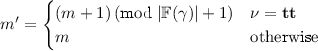
  • (d) $\nu ' = \Bigg \{\begin{array}{ll} \psi _{m'} &{} \qquad \nu = \mathbf {tt}\\ \nabla (\nu ,\varepsilon )\vee \psi _{m} &{} \qquad \mathrm {otherwise}\\ \end{array}$

    where $\{ \mathbf {F}\psi _1,.\,.\,,\mathbf {F}\psi _k\}$ is an enumeration of , $\psi _0 = \mathbf {tt}$ and $\varepsilon = (\sigma ,\pi )$

• $\blacksquare$ I is all states of the form $(\varphi ,\mathbf {tt},\pi ,0)$

• $\blacksquare$ F is all states of the form $(\mu ,\mathbf {tt},\pi ,0)$ where $\beta (\pi ) = \emptyset$, $\mu \ne \mathbf {ff}$, $\mu$ is ex-free

We state the correctness result here and include the proofs in the technical report [9].

Theorem 1

For $\varphi \in \mathrm {LTL}$, $\mathcal {D}(\varphi )$ is a limit deterministic automaton such that $L(\mathcal {D}(\varphi )) = [\![\varphi ]\!]$ and $\mathcal {D}(\varphi )$ is of size at most double exponential in $\varphi$.

The number of different formulae in $\mathcal {B}^+(\varphi )$, is at most double exponential in the size of $\varphi$, since each can be represented as a collection of subsets of subformulae of $\varphi$. $\varPi (\varphi )$ is simply tripartition of $\mathcal {C}(\varphi )$ which is bounded above by $3^{| \varphi |}$. And the counter can take different values which is $\le | \varphi |$. The entire state space ${\mathcal {B}^+(\varphi ) \times \mathcal {B}^+(\varphi ) \times \varPi (\varphi ) \times [{n}]}$ is upper bounded by the product of these which is clearly doubly exponential.

Fig. 3.

Our construction for $\varphi = \mathbf {G}(a{\mathbin {\mathbf {U}}}b)$.

We illustrate our construction using $\varphi = \mathbf {G}(a{\mathbin {\mathbf {U}}}b)$ which is a formula outside $\mathrm {LTL}{}{\setminus }{G}{U}$. The automaton for $\varphi$ is shown in Fig. 3. First note that the $\mathcal {C}(\varphi ) = \{ \varphi ,\mathbf {F}b\}$. Next, observe that the only interesting FG-prediction is $\pi$ in which $\alpha = \{ \varphi \}$, $\beta = \emptyset$ and $\gamma =\{ \mathbf {F}b\}$. This is because any initial state will have $\mu = \varphi$ which forces $\varphi \in \alpha$, and since predictions in $\alpha$ don’t change, every reachable state will have $\varphi \in \alpha$ as well. As for $\mathbf {F}b$ note that the corresponding internal until $a{\mathbin {\mathbf {U}}}b$ will become $\mathbf {ff}$ if $\mathbf {F}b$ is in $\alpha$ and thus making the derivative $\mathbf {ff}$ ($a{\mathbin {\mathbf {U}}}b$ is added to the obligation at each step since $\varphi \in \alpha$ and rule (b)). Therefore $\mathbf {F}b$ cannot be in $\alpha$, and it cannot be in $\beta$ because then it would be eventually in $\alpha$. So $\mathbf {F}b$ has to be in $\gamma$. Now that $\pi$ is fixed, and given input $\sigma$, the obligation $\mu$ changes according to rule (b) as $\mu ' = \nabla (\mu \wedge (a{\mathbin {\mathbf {U}}} b),(\sigma ,\pi ))$. Similarly the carry $\nu$ changes to b if $\nu = \mathbf {tt}$ (as in $q_3$ to $q_1/q_2$) and becomes $\nu ' = \nabla (\nu ,(\sigma ,\pi ))\vee b$ otherwise in accordance with rule (d). The initial state is $q_0$ with $\mu = \varphi$, $\nu =\mathbf {tt}$ and counter $=0$. The counter is incremented whenever $\nu$ becomes $\mathbf {tt}$. It is easy to see that the automaton indeed accepts $\mathbf {G}(a\mathbin {\mathbf {U}}b)$ and is limit deterministic.

4 Efficiency

In this section we state the results regarding the efficiency of our construction for $\mathrm {LTL}_\mathrm{D}$. We prove that there are only exponentially many reachable states in $\mathcal {D}(\varphi )$. A state $q = (\mu ,\nu ,\pi ,n)$ of $\mathcal {D}(\varphi )$ is called reachable if there exists a valid finite run of the automaton that ends in q. A $\mu$ is said to be reachable if $(\mu ,\nu ,\pi ,n)$ is reachable for some choice of $\nu$, $\pi$ and n. Similarly for $\nu$. We show that the space of reachable $\mu$ and $\nu$ is only exponentially large in the size of $\varphi$. Our approach will be to show that every reachable $\mu$ (or $\nu$) can be expressed in a certain way, and we will count the number of different such expressions to obtain an upper bound. The expression for $\mu$ and $\nu$ relies on them being represented in DNF form and uses the syntactic definition of the derivative given in the technical report [9]. Therefore we state only the main result and its consequence on the model checking complexity here and present the proofs in [9].

Theorem 2

For $\varphi \in \mathrm {LTL}_\mathrm{D}$ the number of reachable states in the $\mathcal {D}(\varphi )$ is at most exponential in $| \varphi |$.

Theorem 3

The model checking problem for MDPs against specification in $\mathrm {LTL}_\mathrm{D}$ is EXPTIME-complete

Proof

The upper bound follows from our construction being of exponential size and the fact that the model checking of MDPs can be done by performing a linear time analysis of the synchronous product of the MDP and the automaton [4]. The $\text {EXPTIME}$ hardness lower bound is from the fact that the problem is $\text {EXPTIME}$ hard for the subfragment $\mathrm {LTL}{}{\setminus }{G}{U}$ as proved in [8].

5 Expressive Power of $\mathrm {LTL}_\mathrm{D}$

In this section we show that $\mathrm {LTL}_\mathrm{D}$ is semantically more expressive than $\mathrm {LTL}{}{\setminus }{G}{U}$. We demonstrate that the formula $\varphi _0 = \mathbf {G}(p \vee (q \mathbin {\mathbf {U}}r))$ which is expressible in $\mathrm {LTL}_\mathrm{D}$, cannot be expressed by any formula in $\mathrm {LTL}{}{\setminus }{G}{U}$.

Let us fix integers $\ell ,k\in \mathbb {N}$. We will use $\mathrm {LTL}_{\ell }(F,G)$ to denote the subfragment of $\mathrm {LTL}({{F}}{,}{G})$ where formulae have maximum height $\ell$. Since $\mathbf {X}$ distributes over all other operators we assume that all the $\mathbf {X}$s are pushed inside. We use $\mathrm {LTL}_{\ell ,k}{\setminus } GU$ to denote the fragment where formulae are built out of $\mathbin {\mathbf {U}}$, $\wedge$, $\vee$ and $\mathrm {LTL}_{\ell }(F,G)$ formulae such that the number of $\mathbin {\mathbf {U}}$s used is at most k.

Next, consider the following strings over $2^P$ where $P = \{ p,q,r\}$:

The observation we make is that $\sigma$ satisfies $\varphi _0$ but $\eta _k$ does not. We state the main theorem and the corollary here and leave the details in the tech report [9].

Theorem 4

$\forall \,\varphi \in \mathrm {LTL}_{\ell ,k}{\setminus } GU\quad \sigma \vDash \varphi \implies \eta _k\vDash \varphi$

Corollary 1

$\varphi _0$ is not expressible in $\mathrm {LTL}_{\ell ,k}{\setminus } GU$. Also since $\ell$ and k are arbitrary, $\varphi _0$ is not expressible in $\mathrm {LTL}{}{\setminus }{G}{U}$.

6 Experimental Results

We present our tool Büchifier (available at [1]) that implements the techniques described in this paper. Büchifier is the first tool to generate LDBA with provable exponential upper bounds for a large class of $\mathrm {LTL}$ formulae. The states $(\mu ,\nu ,\pi ,n)$ in our automaton described in Definition 10, involve $\mu ,\nu \in \mathcal {B}^+(\varphi )$ which are essentially sets of sets of subformulae. We view each subformula as a different proposition. We then interpret the formulae in $\mathcal {B}^+(\varphi )$ as a Boolean function on these propositions. In Büchifier we represent these Boolean functions symbolically using Binary Decision Diagrams (BDD). Our overall construction follows a standard approach where we begin with an initial set of states and keep adding successors to discover the entire reachable set of states. We report the number of states, number of transitions and the number of final states for the limit deterministic automata we construct.

Table 1. A Comparison between the sizes of automata produced by Büchifier, Rabinizer 3 and ltl2ldba on various formulae. Column St denotes the number of states, column Tr denotes the number of transitions and column AC denotes the size of the acceptance condition. Entries marked as “–” indicate that the tool failed to construct the automaton and/or the acceptance condition due to the memory limit (1 GB) being exceeded.

MDP model checkers like PRISM [15], for a long time have used the translation from LTL to deterministic Rabin automata and only recently [20] have started using limit deterministic Büchi automata. As a consequence we compare the performance of our method against Rabinizer 3 [12] (the best known tool for translating LTL to deterministic automata) and ltl2ldba [20] (the only other known tool for translating LTL to LDBA). Rabinizer 3 constructs deterministic Rabin automata with generalized Rabin pairs (DGRA). The experimental results in [5, 12] report the size of DGRA using the number of states and number of acceptance pairs of the automata; the size of each Rabin pair is, unfortunately, not reported. Since the size of Rabin pairs influences the efficiency of MDP model checking, we report it here to make a meaningful comparison. We take the size of a Rabin pair to be simply the number of transitions in it. The tool ltl2ldba generates transition-based generalized Büchi automata (TGBA). The experimental results in [20] report the size of the TGBA using number of states and number of acceptance sets, and once again the size of each of these sets is not reported. Since their sizes also effect the model checking procedure we report them here. We take the size of an acceptance set to be simply the number of transitions in it. In Table 1 we report a head to head to comparison of Büchifier, Rabinizer 3 and ltl2ldba on various $\mathrm {LTL}$ formulae.

• 1. The first 5 formulae are those considered in [5]; they are from the GR(1) fragment [18] of $\mathrm {LTL}$. These formulae capture Boolean combination of fairness conditions for which generalized Rabin acceptance is particularly well suited. Rabinizer 3 does well on these examples, but Büchifier is not far behind its competitors. The formulae are instantiations of the following templates: $g_0(j) = \wedge _{i=1}^j (\mathbf {G}\mathbf {F}a_i \Rightarrow \mathbf {G}\mathbf {F}b_i)$, $g_1(j) = \wedge _{i=1}^j (\mathbf {G}\mathbf {F}a_i \Rightarrow \mathbf {G}\mathbf {F}a_{i+1})$.

• 2. The next 5 formulae are also from [5] to show how Rabinizer 3 can effectively handle $\mathbf {X}$s. Büchifier has a comparable number of states and much smaller acceptance condition when compared to Rabinizer 3 and ltl2ldba in all these cases. $\varphi _1 = \mathbf {G}(q \vee \mathbf {X}\mathbf {G}p) \wedge \mathbf {G}(r \vee \mathbf {X}\mathbf {G}\lnot p)$, $\varphi _2 = (\mathbf {G}\mathbf {F}(a \wedge \mathbf {X}^2 b) \vee \mathbf {F}\mathbf {G}b) \wedge \mathbf {F}\mathbf {G}(c \vee (\mathbf {X}a \wedge \mathbf {X}^2 b))$, $\varphi _3 = \mathbf {G}\mathbf {F}(\mathbf {X}^3 a \wedge \mathbf {X}^4 b) \wedge \mathbf {G}\mathbf {F}(b \vee \mathbf {X}c) \wedge \mathbf {G}\mathbf {F}(c \wedge \mathbf {X}^2 a)$, $\varphi _4 = (\mathbf {G}\mathbf {F}a \vee \mathbf {F}\mathbf {G}b) \wedge (\mathbf {G}\mathbf {F}c \vee \mathbf {F}\mathbf {G}(d \vee \mathbf {X}e))$, $\varphi _5 = (\mathbf {G}\mathbf {F}(a \wedge \mathbf {X}^2 c) \vee \mathbf {F}\mathbf {G}b) \wedge (\mathbf {G}\mathbf {F}c \vee \mathbf {F}\mathbf {G}(d \vee (\mathbf {X}a \wedge \mathbf {X}^2 b)))$.

• 3. The next 15 formulae (4 groups) express a variety of natural properties, such as $\mathbf {G}(\textit{req} \Rightarrow \mathbf {F}\textit{ack})$ which says that every request that is received is eventually acknowledged. As shown in the table in many of the cases Rabinizer 3 runs out of memory (1 GB) and fails to produce an automaton, and ltl2ldba fails to scale in comparison with Büchifier. The formulae in the table are instantiations of the following templates: $f_0(j) = \mathbf {G}(\wedge _{i=1}^j(a_i \Rightarrow \mathbf {F}b_i))$, $f_1(j) = \mathbf {G}(\wedge _{i=1}^j(a_i \Rightarrow (\mathbf {F}b_i \wedge \mathbf {F}c_i)))$, $f_2(j) = \mathbf {G}(\vee _{i=1}^j(a_i \wedge \mathbf {G}b_i))$, $f_3(j) = \mathbf {G}(\vee _{i=1}^j(a_i \wedge \mathbf {F}b_i))$.

• 4. The next 6 formulae expressible in $\mathrm {LTL}{}{\setminus }{G}{U}$, contain multiple $\mathbf {X}$s and external $\mathbin {\mathbf {U}}$s. Büchifier constructs smaller automata and is able to scale better than ltl2ldba in these cases as well. The formulae are instantiations of: $h(m,n) = (\mathbf {X}^m p) \mathbin {\mathbf {U}}(q \vee (\wedge _{i=1}^n (a_i \mathbin {\mathbf {U}}\mathbf {X}^m b_i)))$.

• 5. The last few examples are from outside of $\mathrm {LTL}{}{\setminus }{G}{U}$. The first three are in $\mathrm {LTL}_\mathrm{D}$ while the rest are outside $\mathrm {LTL}_\mathrm{D}$. We found that Büchifier did better only in a few cases (like $\psi _3$), this is due to the multiplicative effect that the internal untils have on the size of the automaton. So there is scope for improvement and we believe there are several optimizations that can be done to reduce the size in such cases and leave it for future work. $\psi _1 = \mathbf {F}\mathbf {G}((a \wedge \mathbf {X}^2 b \wedge \mathbf {G}\mathbf {F}b) \mathbin {\mathbf {U}}(\mathbf {G}(\mathbf {X}^2\lnot c\vee \mathbf {X}^2(a \wedge b))))$, $\psi _2 = \mathbf {G}(\mathbf {F}\lnot a \wedge \mathbf {F}(b \wedge \mathbf {X}c) \wedge \mathbf {G}\mathbf {F}(a \mathbin {\mathbf {U}}d))$, $\psi _3 = \mathbf {G}((\mathbf {X}^3 a) \mathbin {\mathbf {U}}(b \vee \mathbf {G}c))$, $\psi _4 = \mathbf {G}((a \mathbin {\mathbf {U}}b) \vee (c \mathbin {\mathbf {U}}d))$, $\psi _5 = \mathbf {G}(a \mathbin {\mathbf {U}}(b \mathbin {\mathbf {U}}(c \mathbin {\mathbf {U}}d)))$.

7 Conclusion

In this paper we presented a translation of formulas in $\mathrm {LTL}$ to limit deterministic automata, generalizing the construction from [8]. While the automata resulting from the translation can, in general, be doubly exponential in the size of the original formula, we observe that for formulas in the subfragment $\mathrm {LTL}_\mathrm{D}$, the automaton is guaranteed to be only exponential in size. The logic $\mathrm {LTL}_\mathrm{D}$ is a more expressive fragment than $\mathrm {LTL}{}{\setminus }{G}{U}$, and thus our results enlarge the fragment of $\mathrm {LTL}$ for which small limit deterministic automata can be constructed. One consequence of our results here is a new $\text {EXPTIME}$ algorithm for model checking MDPs against $\mathrm {LTL}_\mathrm{D}$ formulas, improving the previously known upper bound of $\mathrm {2EXPTIME}$.

Our results in this paper, however, have not fully settled the question of when exponential sized limit deterministic automata can be constructed. We do not believe $\mathrm {LTL}_\mathrm{D}$ to be the largest class. For example, our construction yields small automata for $\varphi = \mathbf {G}(\vee _i (p_i \mathbin {\mathbf {U}}q_i))$, where $p_i,q_i$ are propositions. $\varphi$ is not expressible in $\mathrm {LTL}_\mathrm{D}$. Of course we cannot have an exponential sized construction for full $\mathrm {LTL}$ as demonstrated by the double exponential lower bound in [20].

References

Alur, R., La Torre, S.: Deterministic generators and games for LTL fragments. ACM Trans. Comput. Logic 5(1), 1–25 (2004)
Babiak, T., Blahoudek, F., Křetínský, M., Strejček, J.: Effective translation of LTL to deterministic Rabin automata: beyond the (F,G)-fragment. In: Hung, D., Ogawa, M. (eds.) ATVA 2013. LNCS, vol. 8172, pp. 24–39. Springer, Heidelberg (2013). doi:10.1007/978-3-319-02444-8_4
Courcoubetis, C., Yannakakis, M.: The complexity of probabilistic verification. J. ACM 42(4), 857–907 (1995)
Esparza, J., Křetínský, J.: From LTL to deterministic automata: a safraless compositional approach. In: Biere, A., Bloem, R. (eds.) CAV 2014. LNCS, vol. 8559, pp. 192–208. Springer, Cham (2014). doi:10.1007/978-3-319-08867-9_13
Hahn, E.M., Li, G., Schewe, S., Turrini, A., Zhang, L.: Lazy probabilistic model checking without determinisation. In: CONCUR, pp. 354–367 (2015)
Henzinger, T.A., Piterman, N.: Solving games without determinization. In: Ésik, Z. (ed.) CSL 2006. LNCS, vol. 4207, pp. 395–410. Springer, Heidelberg (2006). doi:10.1007/11874683_26
Kini, D., Viswanathan, M.: Limit deterministic and probabilistic automata for \(\text{ LTL }{\setminus }\text{ GU }\). In: Baier, C., Tinelli, C. (eds.) TACAS 2015. LNCS, vol. 9035, pp. 628–642. Springer, Heidelberg (2015). doi:10.1007/978-3-662-46681-0_57
Kini, D., Viswanathan, M.: Optimal translation of LTL to limit deterministic automata. Technical report, University of Illinois at Urbana-Champaign (2017). http://hdl.handle.net/2142/95004
Klein, J., Baier, C.: Experiments with deterministic \(\omega \)-automata for formulas of linear temporal logic. Theor. Comput. Sci. 363(2), 182–195 (2006)
Klein, J., Müller, D., Baier, C., Klüppelholz, S.: Are good-for-games automata good for probabilistic model checking? In: Dediu, A.-H., Martín-Vide, C., Sierra-Rodríguez, J.-L., Truthe, B. (eds.) LATA 2014. LNCS, vol. 8370, pp. 453–465. Springer, Cham (2014). doi:10.1007/978-3-319-04921-2_37
Komárková, Z., Křetínský, J.: Rabinizer 3: safraless translation of LTL to small deterministic automata. In: Cassez, F., Raskin, J.-F. (eds.) ATVA 2014. LNCS, vol. 8837, pp. 235–241. Springer, Cham (2014). doi:10.1007/978-3-319-11936-6_17
Křetínský, J., Esparza, J.: Deterministic automata for the (F,G)-fragment of LTL. In: Madhusudan, P., Seshia, S.A. (eds.) CAV 2012. LNCS, vol. 7358, pp. 7–22. Springer, Heidelberg (2012). doi:10.1007/978-3-642-31424-7_7
Křetínský, J., Garza, R.L.: Rabinizer 2: small deterministic automata for \(\text{ LTL }{\setminus }\text{ GU }\). In: Hung, D., Ogawa, M. (eds.) ATVA 2013. LNCS, vol. 8172, pp. 446–450. Springer, Heidelberg (2013). doi:10.1007/978-3-319-02444-8_32
Kwiatkowska, M., Norman, G., Parker, D.: PRISM 4.0: verification of probabilistic real-time systems. In: Gopalakrishnan, G., Qadeer, S. (eds.) CAV 2011. LNCS, vol. 6806, pp. 585–591. Springer, Heidelberg (2011). doi:10.1007/978-3-642-22110-1_47
Morgenstern, A., Schneider, K.: From LTL to symbolically represented deterministic automata. In: Logozzo, F., Peled, D.A., Zuck, L.D. (eds.) VMCAI 2008. LNCS, vol. 4905, pp. 279–293. Springer, Heidelberg (2008). doi:10.1007/978-3-540-78163-9_24
Piterman, N., Pnueli, A., Sa’ar, Y.: Synthesis of reactive(1) designs. In: VMCAI, pp. 279–293 (2006)
Piterman, N., Pnueli, A., Sa’ar, Y.: Synthesis of reactive(1) designs. In: Emerson, E.A., Namjoshi, K.S. (eds.) VMCAI 2006. LNCS, vol. 3855, pp. 364–380. Springer, Heidelberg (2005). doi:10.1007/11609773_24
Puterman, M.L.: Markov Decision Processes. Wiley, Hoboken (1994)
Sickert, S., Esparza, J., Jaax, S., Křetínský, J.: Limit-deterministic Büchi automata for linear temporal logic. In: Chaudhuri, S., Farzan, A. (eds.) CAV 2016. LNCS, vol. 9780, pp. 312–332. Springer, Cham (2016). doi:10.1007/978-3-319-41540-6_17
Sickert, S., Křetínský, J.: MoChiBA: probabilistic LTL model checking using limit-deterministic Büchi automata. In: Artho, C., Legay, A., Peled, D. (eds.) ATVA 2016. LNCS, vol. 9938, pp. 130–137. Springer, Cham (2016). doi:10.1007/978-3-319-46520-3_9
Vardi, M., Wolper, P., Sistla, A.P.: Reasoning about infinite computation paths. In: FOCS (1983)
Vardi, M.Y.: Automatic verification of probabilistic concurrent finite-state programs. In: Proceedings of FOCS, pp. 327–338 (1985)
Author information
Authors and Affiliations
Corresponding author
Editor information
Editors and Affiliations
Rights and permissions
Copyright information
© 2017 Springer-Verlag GmbH Germany
About this paper
Cite this paper
Kini, D., Viswanathan, M. (2017). Optimal Translation of LTL to Limit Deterministic Automata. In: Legay, A., Margaria, T. (eds) Tools and Algorithms for the Construction and Analysis of Systems. TACAS 2017. Lecture Notes in Computer Science(), vol 10206. Springer, Berlin, Heidelberg. https://doi.org/10.1007/978-3-662-54580-5_7
Download citation
DOI: https://doi.org/10.1007/978-3-662-54580-5_7
Published:
Publisher Name: Springer, Berlin, Heidelberg
Print ISBN: 978-3-662-54579-9
Online ISBN: 978-3-662-54580-5
eBook Packages: Computer ScienceComputer Science (R0)