
Abstract
In this chapter, we present a theory of traffic breakdown at highway bottlenecks in the framework of the three-phase theory.
This is a preview of subscription content, log in via an institution.
Buying options
Tax calculation will be finalised at checkout
Purchases are for personal use only
Learn about institutional subscriptionsNotes
- 1.
In the theoretical definition of the breakdown probability P (B)(q sum) (5.7), we assume that the flow rate q sum does not depend on time during the time interval T ob. In contrast, in real field traffic data the flow rate is a very complex time-function. For this reason, in the empirical definition of the flow-rate dependence of the probability of spontaneous traffic breakdown at the bottleneck P (B)(q i ) (2.1) (see Figs. 2.2 and 2.3 of Sect. 2.3), rather than the time interval T ob, we should use an averaging time interval for traffic variables T av. A comparison of the theoretical and empirical definitions of the flow-rate dependence of the probability of spontaneous traffic breakdown at a bottleneck has been considered in Sec. 10.3.1 of the book [17].
- 2.
- 3.
For simplicity of this qualitative consideration, we neglect here a complex spatiotemporal dynamics of the permanent local speed disturbance, which will be discussed in Sect. 5.13.
- 4.
Obviously, formula (5.12) can be rewritten as follows (this equivalent form for formula (5.12) has been used in [47]; see caption to Fig. 18 of [47]):
$$\displaystyle\begin{array}{rcl} P^{\mathrm{(B)}}(q_{\mathrm{sum}}) = \left (1 +\mathrm{ tanh}[\chi (q_{\mathrm{sum}} - q_{\mathrm{ P}})]\right )/2,& & {}\\ \end{array}$$where χ = β∕2.
- 5.
For an on-ramp bottleneck (Fig. 5.1a), in (5.12) parameters q P and β depend on the on-ramp inflow rate q on, the flow rate q sum = q on + q in is the flow rate in free flow downstream of the bottleneck, where q in is the flow rate in free flow on the main road upstream of the bottleneck. For the off-ramp bottleneck (Fig. 5.2a), in (5.12) parameters q P and β depend on the percentage of vehicles leaving the main road to off-ramp at an off-ramp bottleneck η off = (q off∕q in)100%, the flow rate q sum = q in, q off is the flow rate of vehicles leaving the main road to off-ramp at the off-ramp bottleneck [17].
- 6.
Initial values for random function rand() in the model (see Appendix B) are different for different simulation realizations.
- 7.
- 8.
The probability of the spontaneous occurrence of traffic breakdown at a highway bottleneck during a given time interval is calculated from a finite number of different days of the observation of free flow at a highway bottleneck. This is because a calculation of the breakdown probability for an infinite number of different days of the observation of free flow at the bottleneck has no sense for real traffic flow.
- 9.
It should be noted that for 2D steady states of synchronized flow (Fig. 5.15a) we have often used the term “the fundamental hypothesis of three-phase traffic theory” [17, 25]. The term should emphasize the qualitative difference between the fundamental hypothesis of earlier traffic flow theories about a theoretical fundamental diagram of traffic flow, i.e., 1D-curve(s) in the flow–density plane (see a discussion of classical traffic flow models with a theoretical fundamental diagram (1D steady states) of traffic flow in Chap. 4). Thus, the term “fundamental hypothesis of three-phase traffic theory” has a sense only, if a comparison between 2D steady states of synchronized flow of the three-phase theory and 1D steady states of traffic flow (theoretical fundamental diagram) of earlier traffic flow theories is made. To emphasize this comparison, we have also used the term “fundamental diagram approach to traffic flow modeling” in the application to two-phase traffic flow models with 1D steady states of traffic flow.
Fig. 5.15 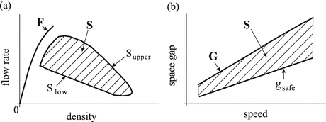
Hypothesis about steady states of synchronized flow in the three-phase theory [2–7]: (a ) Qualitative representation of free flow states (F) and 2D steady states of synchronized flow (dashed region S) on a multi-lane road in the flow–density plane. (b ) A part of the 2D steady states of synchronized flow shown in (a ) in the space-gap–speed plane (dashed region S)
Unfortunately, over last years some of traffic researchers have “extended” the use of the terms “fundamental hypothesis of three-phase traffic theory” and “fundamental diagram approach to traffic flow modelling” behind the above-mentioned comparison. In particular, some of the researchers equalize the three-phase theory and the fundamental hypothesis of three-phase traffic theory. This confusion leads to invalid conclusions and results. For example, while making an assumption that the 2D-states of traffic flow is the main difference between three-phase and two-phase traffic flow models, some of the researchers make an incorrect conclusion that “two-phase traffic models are approximations of the three-phase traffic models”.
For these reasons, in this book we do not use the terms “the fundamental hypothesis of three-phase traffic theory” and “fundamental diagram approach to traffic flow modelling”. Instead of the term “the fundamental hypothesis of three-phase traffic theory”, we use the term “hypothesis of three-phase theory about 2D-states of synchronized flow”. Instead of the term “fundamental diagram approach to traffic flow modelling”, we use the term “two-phase traffic flow models”.
As emphasized in Sect. 1.9, the main reason for the three-phase theory is the explanation of the nucleation nature of traffic breakdown at highway bottlenecks. In other words, the basic assumption of the three-phase theory is the nucleation nature of traffic breakdown at highway bottlenecks, i.e., the explanation of the metastability of free flow with respect to an F → S transition at a highway bottleneck [17, 25]. Moreover, it turns out [38] that (see also Sec. 12.1 of the book [25]), the metastability of free flow with respect to the F → S transition can be explained even if for each vehicle density all synchronized flow states are averaged to one average state. Indeed, even when no 2D-region of steady states of traffic flow it is assumed in a traffic flow model, the metastability of free flow with respect to the F → S transition can be mathematically described in a three-phase model with 1D-region of steady states [38] through a competition between driver speed adaptation to such averaged states of synchronized flow and driver over-acceleration.
- 10.
A more detailed consideration of features of the safe gap g safe, the synchronization space gap G in 2D-region of synchronized flow, related time headway between vehicles (τ safe and τ G), and driver behavioral assumptions explaining this hypothesis can be found in the book [25].
- 11.
Thus, when a vehicle moves initially at a higher speed than the speed of the preceding vehicle and the vehicle cannot overtake the preceding vehicle, then under conditions (5.48) the vehicle decelerates to the speed of the preceding vehicle. Depending on the average value of this vehicle deceleration, we distinguish “strong” speed adaptation and “weak” speed adaptation (see Sect. A.7 of Appendix A) [28]. When the vehicle decelerates quickly to the speed of the preceding vehicle, the average space gap between vehicles remains a large one. This case is called “strong” speed adaptation. Contrarily, when the vehicle adapts its speed slowly to the speed of the preceding vehicle, the average space gap between vehicles becomes a small one. This case is called “weak” speed adaptation. Although in both cases conditions (5.48) are satisfied, features of synchronized flow can be completely different. As shown in [28], under “weak” speed adaptation moving jams emerge easier spontaneously in synchronized flow. In contrast, under “strong” speed adaptation moving jams dissolve usually in synchronized flow (this effect of jam dissolution can also be called “jam absorption”). Because we do not make a comprehensive discussion of spatiotemporal features of congested patterns resulting from the breakdown, a more detailed consideration of “strong” speed adaptation and “weak” speed adaptation [28] is out of the scope of this book.
- 12.
It must be noted that in real traffic flow the speed adaptation and over-acceleration effects appear usually in their dynamic competition within a local disturbance in free flow at a bottleneck. For this reason, a separate consideration of the over-acceleration effect made here is a simplification of the reality (see Sects. 5.12 and 5.13 below).
- 13.
Discrete values of the increase and the decrease in the speed that can be seen in Fig. 5.21d are associated with the discretization of the vehicle acceleration and the speed used in the KKSW CA model (Appendix B).
- 14.
With the exception of this Sect. 5.13, in the book the term F → S transition determines the “completed” F → S transition only. For this reason, we do not used the term “completed” F → S transition any more.
- 15.
To avoid confusions, we do not consider results of simulations of the effect of a moving bottleneck on free flow studied with two-phase traffic flow models. This is because none of the two-phase traffic flow models can show the nucleation nature of traffic breakdown (F → S transition) (Chap. 4). In other words, the two-phase traffic flow models used earlier for a study of the effect of a moving bottleneck on traffic flow (see references in Sect. 1.2) cannot show the theoretical result of this section explaining the nucleation of the breakdown (F → S transition) due to the interaction of one of the waves in free flow with a permanent local speed disturbance localized at a highway bottleneck as found in empirical data (Chap. 3). For this reason, we use the Kerner-Klenov stochastic microscopic model that can explain empirical nucleation features of traffic breakdown in heterogeneous traffic flow [48].
- 16.
- 17.

References
C.W. Gardiner, Handbook of Stochastic Methods, 2nd edn. (Springer, Berlin, 1990)
B.S. Kerner, Phys. Rev. Lett. 81, 3797–3400 (1998)
B.S. Kerner, in Proceedings of the 3rd Symposium on Highway Capacity and Level of Service, ed. by R. Rysgaard, vol. 2 (Road Directorate, Ministry of Transport, Denmark, 1998), pp. 621–642
B.S. Kerner, Trans. Res. Rec. 1678, 160–167 (1999)
B.S. Kerner, in Transportation and Traffic Theory, ed. by A. Ceder (Elsevier Science, Amsterdam, 1999), pp. 147–171
B.S. Kerner, Physics World 12, 25–30 (August 1999)
B.S. Kerner. J. Phys. A Math. Gen. 33, L221–L228 (2000)
B.S. Kerner, in Traffic and Granular Flow ’99: Social, Traffic and Granular Dynamics, ed. by D. Helbing, H.J. Herrmann, M. Schreckenberg, D.E. Wolf (Springer, Heidelberg, Berlin, 2000), pp. 253–284
B.S. Kerner, Transp. Res. Rec. 1710, 136–144 (2000)
B.S. Kerner, Netw. Spat. Econ. 1, 35–76 (2001)
B. S. Kerner, Transp. Res. Rec. 1802, 145–154 (2002)
B. S. Kerner, in Traffic and Transportation Theory in the 21st Century, ed. by M.A.P. Taylor (Elsevier Science, Amsterdam, 2002), pp. 417–439
B.S. Kerner, Phys. Rev. E 65, 046138 (2002)
B. S. Kerner, Math. Comput. Modell. 35, 481–508 (2002)
B.S. Kerner, in Traffic and Granular Flow’ 01, ed. by M. Schreckenberg, Y. Sugiyama, D. Wolf (Springer, Berlin, 2003), pp. 13–50
B.S. Kerner, Physica A 333, 379–440 (2004)
B.S. Kerner, The Physics of Traffic (Springer, Berlin, New York, 2004)
B.S. Kerner, Physica A 355, 565–601 (2005)
B.S. Kerner, in Traffic and Transportation Theory, ed. by H.S. Mahmassani (Elsevier Science, Amsterdam, 2005), pp. 181–203
B.S. Kerner, IEEE Trans. ITS 8, 308–320 (2007)
B.S. Kerner, Transp. Res. Rec. 1999, 30–39 (2007)
B.S. Kerner, Transp. Res. Rec. 2088, 80–89 (2008)
B.S. Kerner, J. Phys. A Math. Theor. 41, 215101 (2008)
B.S. Kerner, in Transportation Research Trends, ed. by P.O. Inweldi. (Nova Science Publishers, New York, 2008), pp. 1–92
B.S. Kerner, Introduction to Modern Traffic Flow Theory and Control (Springer, Heidelberg, Dordrecht, London, New York, 2009)
B.S. Kerner, in Encyclopedia of Complexity and System Science, ed. by R.A. Meyers (Springer, Berlin, 2009), pp. 9302–9355
B.S. Kerner, in Encyclopedia of Complexity and System Science, ed. by R.A. Meyers (Springer, Berlin, 2009), pp. 9355–9411
B.S. Kerner, Phys. Rev. E. 85, 036110 (2012)
B.S. Kerner, Traffic Eng. Contr. 54, 47 (2013)
B.S. Kerner, Physica A 392, 5261–5282 (2013)
B.S. Kerner, Phys. Rev. E 92, 062827 (2015)
B.S. Kerner, in Vehicular Communications and Networks, ed. by W. Chen (Woodhead Publishings, Cambridge, 2015), pp. 223–254
B.S. Kerner, Elektrotechnik Informationstechnik 132, 417–433 (2015)
B.S. Kerner, Physica A 450, 700–747 (2016)
B.S. Kerner, S.L. Klenov, J. Phys. A Math. Gen. 35, L31–L43 (2002)
B.S. Kerner, S.L. Klenov, Phys. Rev. E 68, 036130 (2003)
B.S. Kerner, S.L. Klenov, J. Phys. A Math. Gen. 37, 8753–8788 (2004)
B.S. Kerner, S.L. Klenov, J. Phys. A Math. Gen. 39, 1775–1809 (2006)
B.S. Kerner, S.L. Klenov, Transp. Res. Rec. 1965, 70–78 (2006)
B.S. Kerner, S.L. Klenov, Physica A 364, 473–492 (2006)
B.S. Kerner, S.L. Klenov, Phys. Rev. E 80, 056101 (2009)
B.S Kerner, S.L. Klenov, in Encyclopedia of Complexity and System Science, ed. by R.A. Meyers (Springer, Berlin, 2009), pp. 9282–9302
B.S. Kerner, S.L. Klenov, J. Phys. A Math. Theor. 43, 425101 (2010)
B.S. Kerner, S.L. Klenov, G. Hermanns, M. Schreckenberg, Physica A 392, 4083–4105 (2013)
B.S. Kerner, S.L. Klenov, M. Schreckenberg, Phys. Rev. E 84, 046110 (2011)
B.S. Kerner, S.L. Klenov, M. Schreckenberg, Phys. Rev. E 89, 052807 (2014)
B.S. Kerner, S.L. Klenov, D.E. Wolf, J. Phys. A Math. Gen. 35, 9971–10013 (2002)
B.S. Kerner, M. Koller, S.L. Klenov, H. Rehborn, M. Leibel, Physica A 438, 365–397 (2015)
S.-E. Molzahn, B.S. Kerner, H. Rehborn, S.L. Klenov, M. Koller (unpublished)
Author information
Authors and Affiliations
Rights and permissions
Copyright information
© 2017 Springer-Verlag GmbH Germany
About this chapter
Cite this chapter
Kerner, B.S. (2017). Theoretical Fundamental of Transportation Science—The Three-Phase Theory. In: Breakdown in Traffic Networks. Springer, Berlin, Heidelberg. https://doi.org/10.1007/978-3-662-54473-0_5
Download citation
DOI: https://doi.org/10.1007/978-3-662-54473-0_5
Published:
Publisher Name: Springer, Berlin, Heidelberg
Print ISBN: 978-3-662-54471-6
Online ISBN: 978-3-662-54473-0
eBook Packages: EngineeringEngineering (R0)