
Abstract
Traditional fully homomorphic encryption (FHE) schemes only allow computation on data encrypted under a single key. López-Alt, Tromer, and Vaikuntanathan (STOC 2012) proposed the notion of multi-key FHE, which allows homomorphic computation on ciphertexts encrypted under different keys, and also gave a construction based on a (somewhat nonstandard) assumption related to NTRU. More recently, Clear and McGoldrick (CRYPTO 2015), followed by Mukherjee and Wichs (EUROCRYPT 2016), proposed a multi-key FHE that builds upon the LWE-based FHE of Gentry, Sahai, and Waters (CRYPTO 2013). However, unlike the original construction of López-Alt et al., these later LWE-based schemes have the somewhat undesirable property of being “single-hop for keys:” all relevant keys must be known at the start of the homomorphic computation, and the output cannot be usefully combined with ciphertexts encrypted under other keys (unless an expensive “bootstrapping” step is performed).
In this work we construct two multi-key FHE schemes, based on LWE assumptions, which are multi-hop for keys: the output of a homomorphic computation on ciphertexts encrypted under a set of keys can be used in further homomorphic computation involving additional keys, and so on. Moreover, incorporating ciphertexts associated with new keys is a relatively efficient “native” operation akin to homomorphic multiplication, and does not require bootstrapping (in contrast with all other LWE-based solutions). Our systems also have smaller ciphertexts than the previous LWE-based ones; in fact, ciphertexts in our second construction are simply GSW ciphertexts with no auxiliary data.
C. Peikert—This material is based upon work supported by the National Science Foundation under CAREER Award CCF-1054495 and CNS-1606362, and by the Alfred P. Sloan Foundation. The views expressed are those of the authors and do not necessarily reflect the official policy or position of the National Science Foundation or the Sloan Foundation.
You have full access to this open access chapter, Download conference paper PDF
1 Introduction
Secure multiparty computation (MPC) is an important and well-studied problem in cryptography. In MPC, multiple users want to jointly perform a computation on their respective inputs via an interactive protocol. Informally, the goal is for the protocol to reveal nothing more than the output of the computation.
Fully homomorphic encryption (FHE) is a powerful tool for constructing secure MPC protocols. One approach suggested in Gentry’s seminal work [9], and later optimized by Asharov et al. [4], is to have an initial phase in which all parties run a protocol to generate a sharing of an FHE secret key, then use the public key to encrypt their inputs and publish the ciphertexts. The parties then locally compute an encryption of the output using homomorphic operations. Finally, they run a protocol to decrypt the encrypted output, using their secret key shares. Overall, this approach requires the set of involved parties to be known in advance, and for them to run interactive protocols both before and after their local computation.
López-Alt et al. [15] (hereafter LTV) introduced the interesting notion of on-the-fly MPC, in which the set of parties who contribute inputs to the computation, and even the computation itself, need not be fixed in advance, and can even be chosen adaptively. In addition, there is no interaction among the parties at the outset: any user whose data might potentially be used simply uploads her encrypted input to a central server in advance, and can then go offline. The server then uses the uploaded data to compute (or continue computing) a desired function, and when finished, outputs an encrypted output. Finally, the parties whose inputs were used in the computation—and only those parties—run an interactive protocol to jointly decrypt the ciphertext and obtain the output.
Multi-key FHE. Traditional FHE schemes only allow computation on data encrypted under a single key, and therefore are not suitable for on-the-fly MPC, where users’ inputs must be encrypted under different keys. As a tool for constructing on-the-fly protocols, LTV proposed a new type of FHE scheme, which they called multi-key FHE (MK-FHE). Such a scheme extends the FHE functionality to allow homomorphic computation on ciphertexts encrypted under different, independent keys. Decrypting the result of such a computation necessarily requires all of the corresponding secret keys.
In [15], LTV constructed an MK-FHE scheme based on a variant of the NTRU cryptosystem [13]. Its security was based on a new and somewhat non-standard assumption on polynomial rings, which, unlike the commonly used learning with errors (LWE) assumption [20] or its ring-based analogue [16], is not currently supported by a worst-case hardness theorem.Footnote 1 (LTV also constructed MK-FHE based on ring-LWE, but limited only to a logarithmic number of keys and circuit depth.) Subsequently, Clear and McGoldrick [8] gave an LWE-based construction for an unlimited number of keys, using a variant of the FHE scheme of Gentry et al. [11] (hereafter GSW). Later, Mukherjee and Wichs [18] provided another exposition of the Clear-McGoldrick scheme, and built a two-round (plain) MPC protocol upon it.
Static Versus Dynamic. We observe that the LTV multi-key FHE, to extend the terminology of [10], is “multi-hop for keys,” or, more concisely, “dynamic:” one can perform a homomorphic computation on a collection of ciphertexts encrypted under some set of keys, then use the resulting ciphertext as an input to further homomorphic computation on ciphertexts encrypted under additional keys, and so on. (Multi-hop homomorphic computation is naturally supported by essentially all known single-key FHE schemes as well.) The on-the-fly MPC protocol of [15] naturally inherits this dynamic flavor, which is very much in the spirit of “on the fly” computation, since it allows reusing encrypted results across different computations.
By contrast, it turns out that neither of the MK-FHE constructions from [8, 18] appear to be dynamic, but are instead only static (i.e., single-hop for keys): once a homomorphic computation has been performed on a collection of ciphertexts encrypted under some set of keys, the output cannot easily be used in further computation involving additional keys. Instead, one must restart the whole computation from scratch (incorporating all the relevant keys from the very beginning), or perform an expensive “bootstrapping” step, which may be even more costly.Footnote 2 This rules out a dynamic computation, since all involved parties must be known before the computation begins. In summary, existing constructions of MK-FHE and on-the-fly MPC from standard (worst-case) lattice assumptions still lack basic functionality that has been obtained from more heuristic assumptions.
1.1 Our Results
In this work we construct two (leveled) multi-key FHE schemes, for any number of keys, from LWE assumptions. Like the original MK-FHE scheme of [15], and unlike those of [8, 18], both of our schemes are dynamic (i.e., multi-hop for keys), and hence are suitable for dynamic on-the-fly MPC. Specifically, in our schemes one can homomorphically compute on ciphertexts encrypted under several keys, then use the result in further computation on ciphertexts under additional keys, and so on. Moreover, incorporating ciphertexts associated with new keys into the computation is a relatively efficient “native” operation, akin to GSW ciphertext multiplication, which does not require bootstrapping. In addition, our schemes are also naturally bootstrappable (as usual, under appropriate circular-security assumptions), and can therefore support unbounded homomorphic computations for any polynomial number of keys. We now describe our two systems in more detail, and discuss their different efficiency and security tradeoffs.
Scheme #1: Large Ciphertexts, Standard LWE. The security of our first scheme, which is described in Sect. 3, is based on the standard n-dimensional decision-LWE assumption (appropriately parameterized), but has rather large ciphertexts and correspondingly slow homomorphic operations. Actually, the ciphertexts are about an n factor smaller than fresh ciphertexts in the systems from [8, 18] (see Fig. 1), but unlike in those systems, our ciphertexts remain rather large even after multi-key homomorphic operations. Essentially, this is the price of being dynamic—indeed, it is possible at any point to “downgrade” our ciphertexts to ordinary GSW ciphertexts, by giving up the ability to extend ciphertexts to additional keys.
Scheme #2: Small Ciphertexts, Circular LWE. In our second scheme, which is described in Sect. 4, ciphertexts are simply GSW ciphertexts, and are therefore (relatively) small and admit correspondingly efficient homomorphic operations. This efficiency comes at the price of rather large public keys (which are comparable to fresh ciphertexts in the systems from [8, 18]) and a correspondingly slow algorithm for extending ciphertexts to additional keys. This efficiency profile seems preferable to our first scheme’s, because applications of MK-FHE would typically involve many more homomorphic operations than extensions to new keys. Therefore, we consider this scheme to be our main contribution.
Interestingly, the security of our second scheme appears to require a natural circular security assumption for LWE. Despite some positive results for circular security of LWE-based encryption [3], we do not yet see a way to prove security under standard LWE. We point out, however, that our assumption is no stronger than the circular-security assumptions that are used to “bootstrap” FHE, because any circular-secure FHE is itself fully key-dependent message secure [9]. So in a context where our system is bootstrapped to obtain unbounded FHE, we actually incur no additional assumption.

Properties of LWE-based MK-FHE schemes, where all sizes are in bits. Here k denotes the actual number of secret keys associated with the ciphertext, with a designed upper bound of K; d denotes the boolean circuit depth the scheme is designed to homomorphically evaluate (without bootstrapping); and n is the dimension of the underlying LWE problem used for security. (The \(\tilde{O}\) notation hides logarithmic factors in these parameters.) The arrow \(\rightarrow \) for [8, 18] denotes the change in size following the single “hop” from fresh ciphertexts (under single keys) to multi-key ciphertexts.
Comparison with [6]. A concurrent and independent work by Brakerski and Perlman [6], which also constructs (unbounded) dynamic multi-key FHE from LWE, was posted to ePrint shortly after our original preprint appeared there. (Both works were submitted to CRYPTO’16, but only [6] was accepted.) The construction of Brakerski and Perlman follows the “bootstrapping” approach mentioned above, and is focused on minimizing the ciphertext size. Specifically, their multi-key ciphertexts grow only linearly in the number of secret keys associated with the ciphertext. In addition, they describe an “on-the-fly” bootstrapping algorithm that requires only a linear amount of “local” memory (even though the encrypted secret keys are much larger). However, all this comes at the cost of needing to perform an expensive bootstrapping operation whenever incorporating a ciphertext encrypted under a new key, and also for every homomorphic multiplication/NAND operation. (Essentially, this is because the linear-sized ciphertexts are ordinary LWE vectors, not GSW matrices.)
By contrast, our work gives (leveled) dynamic multi-key FHE schemes for which both homomorphic multiplication and incorporation of new keys are much more efficient “native” operations, requiring only a few standard GSW-style matrix operations. This comes at the cost of relatively larger ciphertexts, which naïvely grow at least quartically in the maximum number of keys (see Fig. 1). However, we point out that using ordinary bootstrapping, our constructions can also be made to support an unbounded number of keys, and with ciphertext sizes that grow only quadratically in the number of associated keys.
1.2 Technical Overview
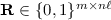
For context, we start with a brief overview of the prior (single-hop for keys) MK-FHE constructions of [8, 18], and the challenge in making them dynamic. In these systems, a fresh ciphertext that decrypts under secret key \(\mathbf {t}\in \mathbb {Z}^{n}\) is a GSW ciphertext \(\mathbf {C}\in \mathbb {Z}_q^{n \times m}\) encrypted to the corresponding public key \(\mathbf {P}\), along with an encryption \(\mathbf {D}\) of the encryption randomness used to produce \(\mathbf {C}\) from \(\mathbf {P}\). (Specifically, each entry of the randomness matrix is encrypted as a separate GSW ciphertext.)
To perform a homomorphic computation on fresh ciphertexts \((\mathbf {C}_{i}, \mathbf {D}_{i})\) that are respectively encrypted under secret keys \(\mathbf {t}_{i}\) for (say) \(i=1,2\), we first extend each ciphertext to an ordinary GSW ciphertext
that decrypts to the same message under the concatenated key \((\mathbf {t}_{1}, \mathbf {t}_{2})\), and then perform normal GSW homomorphic operations on these extended ciphertexts. Essentially, extending \(\mathbf {C}_{1}\) is done by considering the extra “junk” term \((\mathbf {t}_{2}-\mathbf {t}_{1}) \cdot \mathbf {C}_{1}\) that arises from decrypting \(\mathbf {C}_{1}\) under the wrong secret key \(\mathbf {t}_{2}\), and cancelling it out via a ciphertext \(\mathbf {X}_{1}\) that “decrypts” under \(\mathbf {t}_{1}\) to (the negation of) the same junk term. To produce \(\mathbf {X}_{1}\) we use linearly homomorphic operations on \(\mathbf {D}_{1}\) (the encryption of \(\mathbf {C}_{1}\)’s randomness relative to \(\mathbf {P}_{1}\)), along with some additional information about \(\mathbf {t}_{1}\) relative to a shared public parameter.
We point out that in the above scheme, it is not clear how to obtain an encryption of \(\hat{\mathbf {C}}_{i}\)’s underlying encryption randomness—indeed, it is not even clear what composite public key \(\hat{\mathbf {P}}\) the ciphertext \(\hat{\mathbf {C}}_{i}\) would be relative to, nor whether valid encryption randomness for \(\hat{\mathbf {C}}_{i}\) exists at all! (Indeed, for certain natural ways of combining the public keys \(\mathbf {P}_{i}\), valid encryption randomness is not likely to exist.) This is what prevents the extended ciphertexts from satisfying the same invariant that fresh ciphertexts satisfy, which makes the scheme only single-hop for keys. Moreover, even if we could produce an encryption of the ciphertext randomness (assuming it exists), it is not clear whether we could later re-extend an arbitrary ciphertext \(\mathbf {C}\in \mathbb {Z}_q^{2n \times 2m}\) that decrypts under \((\mathbf {t}_{1}, \mathbf {t}_{2})\) to an additional key \(\mathbf {t}_{3}\): the block upper-triangular structure from Eq. (1) would produce a 4n-by-4m matrix, which is too large.
Our Approach. To overcome the above difficulties, our ciphertexts and/or public keys consist of different information, whose invariants can be maintained after extension to additional keys. In particular, we forego maintaining encryption randomness relative to a varying public key, and instead only maintain commitment randomness relative to a fixed public parameter, along with an encryption of that randomness.Footnote 3 Concretely, this works in two different ways in our two schemes, as we now explain.
Scheme #1. In our first system (given in Sect. 3), a ciphertext under a secret key \(\mathbf {t}\in \mathbb {Z}^{kn}\)—which would typically be the concatenation of \(k \ge 1\) individual secret keys—consists of three components:
-
1.
a (symmetric-key) GSW ciphertext \(\mathbf {C}\in \mathbb {Z}_q^{kn \times km}\) that decrypts under \(\mathbf {t}\),
-
2.
a GSW-style homomorphic commitment (à la [12]) \(\mathbf {F}\in \mathbb {Z}_q^{n \times m}\) to the same message, relative to a public parameter, and
-
3.
a special encryption \(\mathbf {D}\) under \(\mathbf {t}\) of the commitment randomness underlying \(\mathbf {F}\).
To extend such a ciphertext to a new secret key \(\mathbf {t}^{*} \in \mathbb {Z}^{n}\), we simply extend the GSW ciphertext \(\mathbf {C}\) to some
where \(\mathbf {X}\) is produced from \(\mathbf {D}\) (in much the same way as above) to cancel out the “junk” term that comes from “decrypting” \(\mathbf {F}\) with \(\mathbf {t}^{*}\). The commitment \(\mathbf {F}\) and its encrypted randomness \(\mathbf {D}\) remain unchanged, except that we need to pad \(\mathbf {D}\) with zeros to make it valid under \((\mathbf {t},\mathbf {t}^{*})\).
Finally, it is not too hard to design homomorphic addition and multiplication operations for ciphertexts having the above form: as shown in [12], GSW commitments admit exactly the same homomorphic operations as GSW encryption, so we can maintain a proper commitment. The homomorphic operations also have a natural, predictable effect on the underlying commitment randomness, so we can use the encrypted randomness \(\mathbf {D}_{i}\) along with the GSW ciphertexts \(\mathbf {C}_{i}\) to maintain correct encrypted commitment randomness.
Scheme #2. Our second system (given in Sect. 4) works differently from all the previous ones. In it, ciphertexts are simply GSW ciphertexts, with no extra components, so they support the standard homomorphic operations. To support extending ciphertexts to additional keys, each public key contains a commitment to its secret key \(\mathbf {t}\), along with an appropriate encryption under \(\mathbf {t}\) of the commitment randomness. (This cyclical relation between secret key and commitment randomness is what leads to our circular-security assumption.) We show how to combine two public keys to get a ciphertext, under the concatenation of their secret keys \(\mathbf {t}_{1}, \mathbf {t}_{2}\), that encrypts the tensor product \(\mathbf {t}_{1} \otimes \mathbf {t}_{2}\) of those keys. By applying homomorphic operations, it is then fairly straightforward to extend a ciphertext that decrypts under one of the keys to a ciphertext that decrypts under their concatenation.
2 Preliminaries
In this work, vectors are denoted by lower-case bold letters (e.g., \(\mathbf {a}\)), and are row vectors unless otherwise indicated. Matrices are denoted by upper-case bold letters (e.g., \(\mathbf {A}\)). We define  for any non-negative integer k.
Approximations. As in many works in lattice cryptography, we work with “noisy equations” and must quantify the quality of the approximation. For this purpose we use the notation \(\approx \) to indicate that the two sides are approximately equal up to some additive error, and we always include a bound on the magnitude of this error. For example,
means that \(x = y + e\) for some \(e \in [-E,E]\). In the case of vectors or matrices, the error bound applies to every entry of the error term, i.e., it is an \(\ell _{\infty }\) bound.
For simplicity of analysis, in this work we use the following rather crude “expansion” bounds to quantify error growth. (Sharper bounds can be obtained using more sophisticated tools like subgaussian random variables.) Because  and
and  , we have implications like

for any \(\mathbf {X}, \mathbf {Y}, \mathbf {R}\).
Tensor Products. The tensor (or Kronecker) product \(\mathbf {A}\otimes \mathbf {B}\) of an \(m_{1}\)-by-\(n_{1}\) matrix \(\mathbf {A}\) with an \(m_{2}\)-by-\(n_{2}\) matrix \(\mathbf {B}\), both over a common ring \(\mathcal {R}\), is the \(m_{1} m_{2}\)-by-\(n_{1} n_{2}\) matrix consisting of \(m_{2}\)-by-\(n_{2}\) blocks, whose (i, j)th block is \(a_{i,j} \cdot \mathbf {B}\), where \(a_{i,j}\) denotes the (i, j)th entry of \(\mathbf {A}\).
It is clear that
for any scalar \(r \in \mathcal {R}\). We extensively use the mixed-product property of tensor products, which says that
for any matrices \(\mathbf {A}, \mathbf {B}, \mathbf {C}, \mathbf {D}\) of compatible dimensions. In particular,
2.1 Cryptographic Definitions
Definition 1
A leveled multi-hop, multi-key FHE scheme is a tuple of efficient randomized algorithms \((\mathsf {Setup}, \mathsf {Gen}, \mathsf {Enc}, \mathsf {Dec}, \mathsf {EvalNAND})\) having the following properties:
-
\(\mathsf {Setup} (1^\lambda , 1^k,1^d)\), given the security parameter \(\lambda \), a bound k on the number of keys, and a bound d on the circuit depth, outputs a public parameter \(pp\). (All the following algorithms implicitly take \(pp\) as an input.)
-
\(\mathsf {Gen} ()\) outputs a public key \(pk\) and secret key \(sk\).
-
\(\mathsf {Enc} (pk, \mu )\), given a public key \(pk\) and a message
 , outputs a ciphertext c. For convenience, we assume that c implicitly contains a reference to \(pk\).
 -
\(\mathsf {Dec} ((sk_1, sk_2, \ldots , sk_t),c)\), given a tuple of secret keys \(sk_1, \ldots , sk_t\) and a ciphertext c, outputs a bit.
-
\(\mathsf {EvalNAND} (c_1,c_2)\), given two ciphertexts \(c_1,c_2\), outputs a ciphertext \(\hat{c}\). For convenience, we assume that \(\hat{c}\) implicitly contains a reference to each public key associated with either \(c_{1}\) or \(c_{2}\) (or both).
 , outputs a ciphertext c. For convenience, we assume that c implicitly contains a reference to
 These algorithms should satisfy correctness and compactness functionality properties, as defined below.
We now describe how to homomorphically evaluate a given boolean circuit composed of NAND gates and having one output wire, which is without loss of generality. The algorithm \(\mathsf {Eval} (C, (c_{1}, \ldots , c_{N}))\), given a circuit C having N input wires, first associates \(c_{i}\) with the ith input wire for each \(i=1,\ldots ,N\). Then for each gate (in some topological order) having input wires i, j and output wire k, it computes \(c_{k} \leftarrow \mathsf {EvalNAND} (c_{i},c_{j})\). Finally, it outputs the ciphertext associated with the output wire.
We stress that the above homomorphic evaluation process is qualitatively different from the ones defined in [15, 18], because when homomorphically evaluating each gate we can only use the key(s) associated with the input ciphertexts for that gate alone; this is what makes the computation multi-hop. By contrast, homomorphic evaluation in [15, 18] is given all the input ciphertexts and public keys from the start, so it can (and does, in the case of [18]) use this knowledge before evaluating any gates.
Definition 2 (Correctness)
A leveled multi-hop, multi-key FHE scheme is correct if for all positive integers \(\lambda , k, d\), for every circuit C of depth at most d having N input wires, for every function \(\pi :[N] \rightarrow [k]\) (which associates each input wire with a key pair), and for every  , the following experiment succeeds with \(1-{{\mathrm{negl}}}(\lambda )\) probability: generate a public parameter \(pp\leftarrow \mathsf {Setup} (1^{\lambda }, 1^{k}, 1^{d})\), generate key pairs \((pk_{j}, sk_{j}) \leftarrow \mathsf {Gen} ()\) for each \(j \in [k]\), generate ciphertexts \(c_{i} \leftarrow \mathsf {Enc} (pk_{\pi (i)}, x_{i})\) for each \(i \in [N]\), let \(\hat{c} \leftarrow \mathsf {Eval} (C, (c_{1}, \ldots , c_{N}))\), and finally test whether
where \(\mathsf {Dec} \) is given those secret keys \(sk_{j}\) corresponding to the public keys referenced by \(\hat{c}\).
Definition 3 (Compactness)
A leveled multi-hop, multi-key FHE scheme is compact if there exists a polynomial \(p(\cdot ,\cdot ,\cdot )\) such that in the experiment from Definition 2,  . In other words, the length of \(\hat{c}\) is independent of C and N, but can depend polynomially on \(\lambda \), k, and d.
2.2 Learning with Errors
For a positive integer dimension n and modulus q, and an error distribution \(\chi \) over \(\mathbb {Z}\), the LWE distribution and decision problem are defined as follows. For an \(\mathbf {s}\in \mathbb {Z}^{n}\), the LWE distribution \(A_{\mathbf {s},\chi }\) is sampled by choosing a uniformly random \(\mathbf {a}\leftarrow \mathbb {Z}_q^{n}\) and an error term  , and outputting
  .
.
Definition 4
The decision-LWE\(_{n,q,\chi }\) problem is to distinguish, with non-negligible advantage, between any desired (but polynomially bounded) number of independent samples drawn from \(A_{\mathbf {s},\chi }\) for a single \(\mathbf {s}\leftarrow \chi ^{n}\), and the same number of uniformly random and independent samples over \(\mathbb {Z}_q^{n+1}\).Footnote 4
A standard instantiation of LWE is to let \(\chi \) be a discrete Gaussian distribution (over \(\mathbb {Z}\)) with parameter \(r = 2\sqrt{n}\). A sample drawn from this distribution has magnitude bounded by, say, \(r\sqrt{n} = \varTheta (n)\) except with probability at most \(2^{-n}\). For this parameterization, it is known that LWE is at least as hard as quantumly approximating certain “short vector” problems on n-dimensional lattices, in the worst case, to within \(\tilde{O}(q\sqrt{n})\) factors [20]. Classical reductions are also known for different parameterizations [5, 19].
In this work it will be convenient to use a form of LWE that is somewhat syntactically different from, but computationally equivalent to, the one defined above. Letting \(\mathbf {s}= (-\bar{\mathbf {s}},1) \in \mathbb {Z}^{n}\) where \(\bar{\mathbf {s}} \leftarrow \chi ^{n-1}\), notice that an LWE sample  drawn from \(A_{\bar{\mathbf {s}},\chi }\) is simply a uniformly random vector satisfying

Therefore, decision-LWE\(_{n-1,q,\chi }\) is equivalent to the problem of distinguishing samples having the above form (and in particular, satisfying Eq. (2)) from uniformly random ones.
More generally, for \(\mathbf {s}\in \mathbb {Z}^{n}\) as above and some \(t = {{\mathrm{poly}}}(n)\), we will need to generate uniformly random vectors \(\mathbf {b}\in \mathbb {Z}_q^{tn}\) that satisfy
for some \( \mathbf {e}\leftarrow \chi ^{t}\). This is easily done by concatenating t independent samples from \(A_{\bar{\mathbf {s}}, \chi }\); clearly, the result is indistinguishable from uniform assuming the hardness of decision-LWE\(_{n,q,\chi }\).
2.3 Gadgets and Decomposition
Here we recall the notion of a “gadget” [17], which is used for decomposing \(\mathbb {Z}_q\)-elements—or more generally, vectors or matrices over \(\mathbb {Z}_q\)—into short vectors or matrices over \(\mathbb {Z}\). We also define some new notation that will be convenient for our application.
For simplicity, throughout this work we use the standard “powers of two” gadget vector

The “bit decomposition” function  outputs a binary column vector (over \(\mathbb {Z}\)) consisting of the binary representation of (the canonical representative in
  of) its argument. As such, it satisfies the identity \(\mathbf {g}\cdot \mathbf {g}^{-1}[a] = a\). (This identity explains the choice of notation \(\mathbf {g}^{-1}\); we stress that \(\mathbf {g}^{-1}\) is a function, not a vector itself.) Symmetrically, we define the notation
which outputs a binary row vector and satisfies the identity \([a]\mathbf {g}^{-t} \cdot \mathbf {g}^{t} = a\). (This identity explains why we place the bracketed argument to the left of \(\mathbf {g}^{-t}\).)
More generally, we define the operation denoted by \((\mathbf {I}_{n} \otimes \mathbf {g}^{-1})[\cdot ]\), which applies \(\mathbf {g}^{-1}\) entrywise to a height-n vector/matrix, and thereby produces a height-\(n\ell \) binary output that satisfies the convenient identity
Similarly, we define \([\cdot ](\mathbf {I}_{n} \otimes \mathbf {g}^{-t})\) to apply \(\mathbf {g}^{-t}\) entrywise to a width-n vector/matrix, thereby producing a width-\(n\ell \) output that satisfies
For the reader who is familiar with previous works that use gadget techniques, the matrix \(\mathbf {I}_{n} \otimes \mathbf {g}\) is exactly the n-row gadget matrix \(\mathbf {G}\), and \((\mathbf {I}_{n} \otimes \mathbf {g}^{-1})[\cdot ]\) is exactly the bit-decomposition operation \(\mathbf {G}^{-1}\) on height-n vectors/matrices. In this work we adopt the present notation because we use several different dimensions n, and because it interacts cleanly with tensor products of vectors and matrices, which we use extensively in what follows.
3 Large-Ciphertext Construction
In this section we describe our first construction of a multi-hop, multi-key FHE, which has small keys but rather large ciphertexts (although fresh ciphertexts are still smaller than in prior constructions). For simplicity, we describe the scheme in the symmetric-key setting, but then note how to obtain a public-key scheme using a standard transformation.
The system is parameterized by a dimension n, modulus q, and error distribution \(\chi \) for the underlying LWE problem; we also let  . For concreteness, we let \(\chi \) be the standard discrete Gaussian error distribution with parameter \(2\sqrt{n}\); to recall, the samples it produces have magnitudes bounded by some \(E = \varTheta (n)\) except with exponentially small \(2^{-\varOmega (n)}\) probability. The modulus q is instantiated in Sect. 3.3, based on a desired depth of homomorphic computation and number of distinct keys. The scheme is defined as follows.
-
\(\mathsf {Setup} \): output a uniformly random \(\mathbf {A}\in \mathbb {Z}_q^{n \times m}\).
-
\(\mathsf {Gen} (\mathbf {A})\): choose \(\bar{\mathbf {t}} \leftarrow \chi ^{n-1}\) and define \(\mathbf {t}:= (-\bar{\mathbf {t}}, 1) \in \mathbb {Z}^{n}\). Choose \(\mathbf {e}\leftarrow \chi ^{m}\) and define
$$\begin{aligned} \mathbf {b}&:= \mathbf {t}\mathbf {A}+ \mathbf {e}\nonumber \\&\approx \mathbf {t}\mathbf {A}\in \mathbb {Z}_q^{m}.&(\text {error}\,E) \end{aligned}$$(3)Output \(\mathbf {t}\) as the secret key and \(\mathbf {b}\) as the associated public extension key.
-
 : do the following, outputting \((\mathbf {C},\mathbf {F},\mathbf {D})\) as the ciphertext.
-
1.
As described in Sect. 2.2, choose an LWE matrix \(\bar{\mathbf {C}} \in \mathbb {Z}_q^{n \times n\ell }\) that satisfies \(\mathbf {t}\bar{\mathbf {C}} \approx \mathbf {0}\), and define
$$\begin{aligned} \mathbf {C}:= \bar{\mathbf {C}} + \mu (\mathbf {I}_{n} \otimes \mathbf {g}) \in \mathbb {Z}_q^{n \times n\ell }. \end{aligned}$$Notice that \(\mathbf {C}\) is simply a GSW ciphertext encrypting \(\mu \) under secret key \(\mathbf {t}\):
$$\begin{aligned} \mathbf {t}\mathbf {C}&= \mathbf {t}\bar{\mathbf {C}} + \mu (\mathbf {t}\otimes 1) \cdot (\mathbf {I}_{n} \otimes \mathbf {g}) \approx \mu (\mathbf {t}\otimes \mathbf {g}).&(\text {error}\,E_{\mathbf {C}}) \end{aligned}$$(4) -
2.
In addition, choose a uniformly random
 and define $$\begin{aligned} \mathbf {F}:= \mathbf {A}\mathbf {R}+ \mu (\mathbf {I}_{n} \otimes \mathbf {g}) \in \mathbb {Z}_q^{n \times n\ell }. \end{aligned}$$(5)
We view \(\mathbf {F}\) as a commitment to the message \(\mu \) under randomness \(\mathbf {R}\).
-
3.
Finally, choose (as described in Sect. 2.2) an LWE matrix \(\bar{\mathbf {D}} \in \mathbb {Z}_q^{nm\ell \times n\ell }\) that satisfies
$$\begin{aligned} (\mathbf {I}_{m \ell } \otimes \mathbf {t}) \cdot \bar{\mathbf {D}}&\approx \mathbf {0}, \end{aligned}$$and define \(\mathbf {D}:= \bar{\mathbf {D}} + (\mathbf {R}\otimes \mathbf {g}^{t} \otimes \mathbf {e}_{n}^{t})\), where \(\mathbf {e}_{n} \in \mathbb {Z}^{n}\) is the nth standard basis vector (so \(\mathbf {t}\cdot \mathbf {e}^{t} = 1\)). We therefore have
$$\begin{aligned} (\mathbf {I}_{m \ell } \otimes \mathbf {t}) \cdot \mathbf {D}&\approx \mathbf {R}\otimes \mathbf {g}^{t}.&(\text {error}\,E_{\mathbf {D}}) \end{aligned}$$(6)We view \(\mathbf {D}\) as a kind of encryption of the commitment randomness \(\mathbf {R}\).
-
1.
-
\(\mathsf {Dec} (\mathbf {t}, (\mathbf {C},\mathbf {F},\mathbf {D}))\): this is standard GSW decryption of \(\mathbf {C}\) under \(\mathbf {t}\), which works due to Eq. (4).
 : do the following, outputting
  and define
 Remark 1
The above scheme is defined in the symmetric-key setting, i.e., \(\mathsf {Enc} \) uses the secret key \(\mathbf {t}\) to generate LWE samples. We can obtain a public-key scheme using a standard technique, namely, have the encryption algorithm rerandomize some public LWE samples to generate as many additional samples as needed. More formally, we define \(\mathbf {B}:= \mathbf {A}- \mathbf {e}_n^{t} \otimes \mathbf {b}\). Then because \(\mathbf {t}\cdot \mathbf {e}_n^{t} = 1\), we have
The public-key encryption algorithm then constructs \(\bar{\mathbf {C}}, \bar{\mathbf {D}}\) by generating fresh samples as \(\mathbf {B}\cdot \mathbf {x}\) for fresh uniformly random  . It is easy to verify that \(\mathbf {t}(\mathbf {B}\mathbf {x}) \approx 0\) with error \(m \cdot E\). Security follows from a standard argument, using the LWE assumption to make \(\mathbf {b}\) (and thereby \(\mathbf {B}\)) uniformly random, and then the leftover hash lemma to argue that the distribution of the fresh samples is negligibly far from uniform.
Theorem 1
The above scheme is IND-CPA secure assuming the hardness of the decision-LWE\(_{n-1,q,\chi }\) problem.
Proof
We prove that the view of an attacker in the real game is indistinguishable from its view in a game in which the public extension key and every ciphertext are uniformly random and independent of the message; this clearly suffices for IND-CPA security. We proceed by a considering the following sequence of hybrid experiments:
- Game 0::
-
This is the real IND-CPA game.
- Game 1::
-
In this game the public extension key and the \(\mathbf {C}, \mathbf {D}\) components of every ciphertext are uniformly random and independent (but \(\mathbf {F}\) is constructed in the same way). More precisely:
- 1.:
-
Choose uniformly random public parameter \(\mathbf {A}\) and extension key \(\mathbf {b}\), and give them to the adversary.
- 2.:
-
For each encryption query, choose uniformly random and independent \(\mathbf {C}\in \mathbb {Z}_{q}^{n \times n\ell }\) and \(\mathbf {D}\in \mathbb {Z}_q^{nm\ell \times n\ell }\), construct \(\mathbf {F}\) exactly as in \(\mathsf {Enc} \), and give ciphertext \((\mathbf {C}, \mathbf {F}, \mathbf {D})\) to the adversary.
- Game 2::
-
This is the ideal game; the only change from the previous game is that each \(\mathbf {F}\) is chosen uniformly at random.
We claim that Games 0 and 1 are computationally indistinguishable under the LWE hypothesis. To prove this we describe a simulator \(\mathcal {S}\) that is given an unbounded source of samples; when they are LWE samples it simulates Game 0, and when they are uniformly random samples it simulates Game 1. It works as follows:
-
Draw m samples and form a matrix \(\bar{\mathbf {A}} \in \mathbb {Z}_q^{n \times m}\) with the samples as its columns. Choose a uniformly random extension key \(\mathbf {b}\in \mathbb {Z}_q^{m}\), and let the public parameter \(\mathbf {A}= \bar{\mathbf {A}} + \mathbf {e}_n^{t} \otimes \mathbf {b}\).
-
On encryption query \(\mu \), draw samples to construct matrices \(\bar{\mathbf {C}}\) and \(\bar{\mathbf {D}}\), and define \(\mathbf {C}, \mathbf {D}\) from these as in \(\mathsf {Enc} \). Also construct \(\mathbf {F}\) exactly as in \(\mathsf {Enc} \).
If the simulator’s input distribution is \(A_{\bar{\mathbf {t}},\chi }\) for some \(\bar{\mathbf {t}} \leftarrow \chi ^{n-1}\), then the first \(n-1\) rows of \(\bar{\mathbf {A}}\) are uniformly random, hence \(\mathbf {A}\) is uniformly random by construction. Moreover, \(\mathbf {b}\approx (-\bar{\mathbf {t}},1) \cdot \mathbf {A}\) has the same distribution as in the real game. Finally, \(\bar{\mathbf {C}}\) and \(\bar{\mathbf {D}}\) are constructed exactly as in the real game, so \(\mathcal {S}\) perfectly simulates Game 0.
By contrast, if the simulator’s input distribution is uniform, then \(\mathbf {A}\) and \(\mathbf {b}\) are uniformly random and independent. Similarly, because \(\bar{\mathbf {C}}\) and \(\bar{\mathbf {D}}\) are uniform and independent of everything else, so are \(\mathbf {C}\) and \(\mathbf {D}\). Therefore, \(\mathcal {S}\) perfectly simulates Game 1. This proves the first claim.
Finally, we claim that Games 1 and 2 are statistically indistinguishable. This follows directly from the leftover hash lemma. This concludes the proof.
3.1 Extending Ciphertexts
We first describe how to extend a ciphertext to an additional secret key \(\mathbf {t}^{*}\), using the associated public extension key \(\mathbf {b}^{*} \approx \mathbf {t}^{*} \mathbf {A}\in \mathbb {Z}_q^{m}\). More precisely, suppose we have a ciphertext that encrypts \(\mu \) under secret key \(\mathbf {t}\in \mathbb {Z}^{n'}\). (Here the dimension \(n'\) can be arbitrary, but typically \(n' = nk\) for some positive integer k, and \(\mathbf {t}\) is the concatenation of k individual secret keys, each of dimension n.) The ciphertext therefore consists of component matrices
that satisfy Eqs. (4)–(6) for some short commitment randomness \(\mathbf {R}\in \mathbb {Z}^{m \times n\ell }\). (Notice that the dimensions of \(\mathbf {F}\) and the width of \(\mathbf {D}\) do not depend on \(n'\).)
Our goal is to extend \((\mathbf {C},\mathbf {F},\mathbf {D})\) to a new ciphertext \((\mathbf {C}', \mathbf {F}', \mathbf {D}')\) that satisfies Eqs. (4)–(6) with respect to the concatenated secret key \(\mathbf {t}' = (\mathbf {t}, \mathbf {t}^{*}) \in \mathbb {Z}^{n'+n}\) and some short commitment randomness \(\mathbf {R}'\). We do so as follows.
-
The commitment and its randomness are unchanged: we define \(\mathbf {F}' := \mathbf {F}\) and \(\mathbf {R}' := \mathbf {R}\). This clearly preserves Eq. (5).
-
Similarly, the encrypted randomness also is essentially unchanged, up to some padding by zeros: we define
$$\begin{aligned} \mathbf {D}' := (\mathbf {I}_{m\ell } \otimes \begin{pmatrix} \mathbf {I}_{n'} \\ \mathbf {0}_{n \times n'} \end{pmatrix} ) \cdot \mathbf {D}\in \mathbb {Z}_q^{(n'+n)m\ell \times n\ell }. \end{aligned}$$Then Eq. (6) is preserved: \((\mathbf {I}_{m \ell } \otimes \mathbf {t}') \cdot \mathbf {D}' = (\mathbf {I}_{m \ell } \otimes \mathbf {t}) \cdot \mathbf {D}\approx \mathbf {R}\otimes \mathbf {g}^{t} = \mathbf {R}' \otimes \mathbf {g}^{t}\).
-
Lastly, we define
$$\begin{aligned} \mathbf {C}' := \left( \begin{array}{ll} \mathbf {C}&{} \mathbf {X}\\ &{} \mathbf {F}\end{array} \right) \in \mathbb {Z}_q^{(n'+n) \times (n'+n)\ell } \end{aligned}$$where \(\mathbf {X}\) is defined as follows:
 (7)
(7)

We now do the error analysis for ciphertext extension. Notice that by construction,
Putting everything together, we see that Eq. (4) is preserved:

In total, the error in the new ciphertext \(\mathbf {C}'\) is

We remark that the error growth is merely additive, so we can extend to multiple new keys with only additive error growth per key. This is important for bootstrapping a multi-key ciphertext, where the first step is to extend the circularly encrypted secret keys to the keys that the ciphertext is encrypted under.
3.2 Homomorphic Operations
We now describe homomorphic addition and multiplication for the above cryptosystem. Suppose we have two ciphertexts \((\mathbf {C}_1,\mathbf {F}_1,\mathbf {D}_1)\) and \((\mathbf {C}_2,\mathbf {F}_2,\mathbf {D}_2)\) that respectively encrypt \(\mu _1\) and \(\mu _2\), with commitment randomness \(\mathbf {R}_1\) and \(\mathbf {R}_2\), under a common secret key \(\mathbf {t}\in \mathbb {Z}^{n'}\). (As in the previous subsection, everything below works for arbitrary dimension \(n'\) and key \(\mathbf {t}\), but typically \(n'=nk\) for some positive integer k, and \(\mathbf {t}\) is the concatenation of k individual secret keys.) Recall that the ciphertext components
satisfy Eqs. (4)–(6) for some short commitment randomness \(\mathbf {R}_{i} \in \mathbb {Z}^{m \times n\ell }\).
-
Negation and scalar addition. (These are used to homomorphically compute NAND
 for
for  .) To homomorphically negate a message for a ciphertext \((\mathbf {C}, \mathbf {F}, \mathbf {D})\), just negate each of the components. It is clear that this has the desired effect, and that the associated commitment randomness and error terms are also negated. To homomorphically add a constant \(c \in \mathbb {Z}\) to a message, just add \(c(\mathbf {I}_{n'} \otimes \mathbf {g})\) to both \(\mathbf {C}\) and \(\mathbf {F}\). It is clear that this has the desired effect, and leaves the commitment randomness and error terms unchanged.
 -
Addition. To homomorphically add, we simply add the corresponding matrices, outputting
$$\begin{aligned}\begin{gathered} (\mathbf {C}_{\text {add}},\mathbf {F}_{\text {add}}, \mathbf {D}_{\text {add}}) := (\mathbf {C}_1 + \mathbf {C}_2 ,\mathbf {F}_1 + \mathbf {F}_2, \mathbf {D}_1 + \mathbf {D}_2). \end{gathered}\end{aligned}$$It is easy to verify that Eqs. (4)–(6) hold for the new ciphertext with message \(\mu _{\text {add}} = \mu _{1}+\mu _{2}\) and commitment randomness \(\mathbf {R}_{\text {add}} = \mathbf {R}_1 + \mathbf {R}_2\), where the errors in the approximations are also added.
-
Multiplication. To homomorphically multiply, we define the short matrices
 (8)
(8) (9)
(9) (10)
(10)and output the ciphertext consisting of
$$\begin{aligned} \mathbf {C}_{\text {mul}}&:= \mathbf {C}_{1} \cdot \mathbf {S}_{c} \\ \mathbf {F}_{\text {mul}}&:= \mathbf {F}_{1} \cdot \mathbf {S}_{f} \\ \mathbf {D}_{\text {mul}}&:= \mathbf {D}_{1} \cdot \mathbf {S}_{f} + (\mathbf {I}_{m\ell } \otimes \mathbf {C}_1) \cdot \mathbf {S}_{d}. \end{aligned}$$The associated commitment randomness is defined as
$$\begin{aligned} \mathbf {R}_{\text {mul}} := \mathbf {R}_{1} \cdot \mathbf {S}_{f} + \mu _1 \mathbf {R}_{2}. \end{aligned}$$
 for
for  .) To homomorphically negate a message for a ciphertext


We now show that the ciphertext output by homomorphic multiplication satisfies Eqs. (4)–(6) for key \(\mathbf {t}\), message \(\mu _{\text {mul}} = \mu _{1} \mu _{2}\), and commitment randomness \(\mathbf {R}_{\text {mul}}\). We already know that Eq. (4), the GSW ciphertext relation, is satisfied by construction of \(\mathbf {C}_{\text {mul}}\) as the homomorphic product of GSW ciphertexts \(\mathbf {C}_{1}, \mathbf {C}_{2}\). Specifically:
Similarly, Eq. (5) is satisfied by construction of \(\mathbf {F}_{\text {mul}}\) as the homomorphic product of commitments \(\mathbf {F}_{1}, \mathbf {F}_{2}\):
Finally, to see that Eq. (6) holds for \(\mathbf {D}_{\text {mul}}\), first notice that
In addition,
Summing Eqs. (11) and (12) yields
with error \(n\ell \cdot E_{\mathbf {D}_{1}} + n'\ell \cdot E_{\mathbf {C}_1} + \mu _{1} \cdot E_{\mathbf {D}_2}\) as desired.
3.3 Instantiating the Parameters
We now bound the worst-case error growth when homomorphically evaluating a depth-d circuit of NAND gates for up to k individual keys. As above, let \(n' = nk\). For a ciphertext \((\mathbf {C},\mathbf {F},\mathbf {D})\) with commitment randomness \(\mathbf {R}\), define the “max error”

By the bounds from the previous subsection, for two ciphertexts with max error at most \(E^{*}\), their homomorphic NAND has max error at most \((n(k+1)\ell + 1) \cdot E^{*} = {{\mathrm{poly}}}(n,k,\ell ) \cdot E^{*}\). Similarly, when we extend a ciphertext with max error at most \(E^{*}\), the result has max error at most \((m(\ell + 1) + 1) \cdot E^* = {{\mathrm{poly}}}(n,\ell ) \cdot E^{*}\). Therefore, for any depth-d homomorphic computation on fresh ciphertexts encrypted under k keys, the result has max error at most
The GSW decryption algorithm works correctly on a ciphertext as long as its error is smaller than q / 4, hence it suffices to choose a modulus q that exceeds the above quantity by a factor of four. Recalling that \(\ell = \varTheta (\log q) = \tilde{O}(k+d)\), this corresponds to a worst-case approximation factor of \({{\mathrm{poly}}}(n,k,d)^{k+d}\) for n-dimensional lattice problems.
We also remark that when bootstrapping a k-key ciphertext, we first extend the circularly encrypted secret keys to the k relevant keys, incurring only additive \({{\mathrm{poly}}}(n,k,\ell )\) error growth, then we run the bootstrapping algorithm. Using an algorithm from [2, 7] that incurs only additive \({{\mathrm{poly}}}(n,k,\ell )\) error growth, we can use a modulus q that is as small as slightly super-polynomial \(q=n^{\omega (1)}\) and still support any polynomial number of keys.
4 Smaller-Ciphertext Construction
In this section we describe a multi-hop, multi-key FHE having smaller ciphertexts and more efficient homomorphic operations than the one in Sect. 3. Indeed, ciphertexts in this system are simply GSW ciphertexts (with no additional information), which admit the usual homomorphic operations. These efficiency improvements come at the cost of larger public extension keys, as well as a circular-security assumption.
Recall that in the scheme from the previous section, a ciphertext includes a commitment to the message, along with a special encryption of the commitment randomness. By contrast, in the scheme described below, the extension key contains a commitment to the secret key, along with an encryption (under the secret key) of the commitment randomness. (Using the commitment randomness to hide the secret key, and using the secret key to hide the commitment randomness, is what leads to a circular-security assumption.) We show how to combine two extension keys to get an encryption, under the concatenation of the secret keys, of the tensor product of those keys; this in turn lets us extend a ciphertext encrypted under one of the keys to their concatenation. We now describe the construction.
As in the previous section, the scheme is parameterized by LWE parameters n and q, the standard error distribution \(\chi \) (which is E-bounded for \(E=\varTheta (n)\)), and  . The system is defined as follows.
-
\(\mathsf {Setup} \): output a uniformly random \(\mathbf {A}\in \mathbb {Z}_q^{n \times m}\).
-
\(\mathsf {Gen} (\mathbf {A})\): do the following, outputting \(\mathbf {t}\) as the secret key and \((\mathbf {b}, \mathbf {P}, \mathbf {D})\) as the public extension key.
-
1.
Choose \(\bar{\mathbf {t}} \leftarrow \chi ^{n-1}\) and define \(\mathbf {t}:= (-\bar{\mathbf {t}}, 1) \in \mathbb {Z}^{n}\). Choose \(\mathbf {e}\leftarrow \chi ^{m}\) and define
$$\begin{aligned} \mathbf {b}&:= \mathbf {t}\mathbf {A}+ \mathbf {e}\\&\approx \mathbf {t}\mathbf {A}\in \mathbb {Z}_q^{m}.&\text {(error}\,E) \end{aligned}$$ -
2.
Choose a uniformly random
 and define $$\begin{aligned} \mathbf {P}:= \mathbf {A}\mathbf {R}+ (\mathbf {I}_{n} \otimes \mathbf {t}\otimes \mathbf {g}) \in \mathbb {Z}_q^{n \times n^{2} \ell }. \end{aligned}$$
 -
3.
As described in Sect. 2.2, choose an LWE matrix \(\bar{\mathbf {D}} \in \mathbb {Z}_q^{n m \ell \times n^{2} \ell }\) that satisfies \((\mathbf {I}_{m\ell } \otimes \mathbf {t}) \cdot \bar{\mathbf {D}} \approx \mathbf {0}\) (with error E), and define \(\mathbf {D}:= \bar{\mathbf {D}} + (\mathbf {R}\otimes \mathbf {g}^{t} \otimes \mathbf {e}_{n}^{t})\), where
 denotes the nth standard basis vector. Notice that, because \(\mathbf {t}\cdot \mathbf {e}_{n}^{t} = 1\), we have $$\begin{aligned} (\mathbf {I}_{m \ell } \otimes \mathbf {t}) \cdot \mathbf {D}&\approx \mathbf {R}\otimes \mathbf {g}^{t}.&\text {(error}\,\,E) \end{aligned}$$
-
1.
 and define
  denotes the nth standard basis vector. Notice that, because
 -
 : This is standard GSW encryption. Specifically, as described in Sect. 2.2, choose an LWE matrix \(\bar{\mathbf {C}} \in \mathbb {Z}_q^{n \times n\ell }\) that satisfies \(\mathbf {t}\bar{\mathbf {C}} \approx \mathbf {0}\), and output the ciphertext \(\mathbf {C}:= \bar{\mathbf {C}} + \mu (\mathbf {I}_{n} \otimes \mathbf {g})\). Notice that \(\mathbf {t}\), \(\mathbf {C}\) satisfy the GSW relation $$\begin{aligned} \mathbf {t}\mathbf {C}&= \mathbf {t}\bar{\mathbf {C}} + \mu (\mathbf {t}\otimes 1) \cdot (\mathbf {I}_{n} \otimes \mathbf {g}) \approx \mu (\mathbf {t}\otimes \mathbf {g}).&\text {(error}\,\,E_{\mathbf {C}}) \end{aligned}$$
 -
\(\mathsf {Dec} (\mathbf {t}, \mathbf {C})\): this is standard GSW decryption.
 : This is standard GSW encryption. Specifically, as described in Sect.
 We again stress that ciphertexts in the above system are just GSW ciphertexts (with no auxiliary information), so homomorphic addition and multiplication work as usual (and as in Sect. 3). Therefore, we only need to show how to extend ciphertexts to new keys, which we do below in Sect. 4.1.
For security, we rely on the following circular hardness assumption: that LWE samples for secret \(\bar{\mathbf {t}} \leftarrow \chi ^{n}\) are indistinguishable from uniform, even given \((\mathbf {b}, \mathbf {A}, \mathbf {P}, \mathbf {D})\) as constructed by \(\mathsf {Setup} \) and \(\mathsf {Gen} \) (using secret \(\bar{\mathbf {t}}\)). We remark that this assumption is “circular” because \(\mathbf {D}\) computationally hides (but statistically determines) \(\mathbf {R}\) under \(\bar{\mathbf {t}}\), and \(\mathbf {P}\) hides \(\bar{\mathbf {t}}\) using \(\mathbf {R}\).
The proof of the following theorem follows immediately from the assumption.
Theorem 2
The above scheme is IND-CPA secure under the above circular-security assumption.
Proof
The proof follows immediately from the assumption: in the real IND-CPA game, the adversary gets the public information \((\mathbf {b}, \mathbf {A}, \mathbf {P}, \mathbf {D})\) along with ciphertexts generated from LWE samples with secret \(\bar{\mathbf {t}}\). In the ideal world, these samples are instead uniformly random, and hence perfectly hide the encrypted messages. Indistinguishability of the two worlds follows directly from the circular-security assumption.
4.1 Extending a Ciphertext to a New Key
We now show how to extend a (potentially multi-key) ciphertext to an additional key, so as to preserve the GSW relation for the concatenation of the secret keys. Specifically, suppose we have a ciphertext \(\mathbf {C}\in \mathbb {Z}_q^{n' \times n' \ell }\) that encrypts \(\mu \) under a key \(\mathbf {t}\in \mathbb {Z}^{n'}\), i.e.,
In this setting, \(n' = nk\) for some positive integer \(k \ge 1\), and \(\mathbf {t}= (\mathbf {t}_{1}, \ldots , \mathbf {t}_{k})\) is the concatenation of k individual secret keys \(\mathbf {t}_{i} \in \mathbb {Z}^{n}\) for which we know the associated vector \(\mathbf {b}_{i} \approx \mathbf {t}_{i} \mathbf {A}\in \mathbb {Z}_q^{m}\) (with error E) from the public extension key. (We will not need the extension key’s other components \(\mathbf {P}\), \(\mathbf {D}\).)
We wish to extend \(\mathbf {C}\) to an additional secret key \(\mathbf {t}^{*}\) for which we know the associated matrices \(\mathbf {P}^{*}\), \(\mathbf {D}^{*}\) from the public extension key (we will not need the associated \(\mathbf {b}^{*}\)). More precisely, we want to generate a ciphertext \(\mathbf {C}'\) that encrypts \(\mu \) under \(\mathbf {t}' = (\mathbf {t}, \mathbf {t}^{*}) \in \mathbb {Z}^{n(k+1)}\), i.e., we want
To do this, we output
where  is as defined below. Notice that by construction,
Below we show how to satisfy
with error
which yields \(\mathbf {t}' \mathbf {C}' \approx \mu (\mathbf {t}' \otimes \mathbf {g})\) with error  , as desired.
Remark 2
While the error bound \(E_{\mathbf {C}'} = \mathbf {E}_{\mathbf {C}} \cdot E + {{\mathrm{poly}}}(n,k,\ell )\) is multiplicative in the original error \(E_{\mathbf {C}}\), we can still extend to multiple new keys while incurring just one factor-of-E increase in the error. This is important for bootstrapping a multi-key ciphertext, where the first step is to extend the circularly encrypted secret keys to all the keys that the ciphertext is encrypted under. The method works by naturally generalizing Eq. (13) to a matrix with blocks along the diagonal and top row only.
Constructing \(\mathbf {X}'\). We construct \(\mathbf {X}'\) in two steps:
-
1.
Using just the \(\mathbf {b}_{i}\) and \(\mathbf {P}^{*}\), \(\mathbf {D}^{*}\) (but not the ciphertext \(\mathbf {C}\)), we construct
 that satisfies $$\begin{aligned} \mathbf {t}' \mathbf {Y}'&= \mathbf {t}\mathbf {Y}+ \mathbf {t}^{*} \mathbf {Y}^{*} \approx (\mathbf {t}\otimes \mathbf {t}^{*} \otimes \mathbf {g}) \end{aligned}$$(15)
with error \(E_{\mathbf {Y}'} = (k \ell + 1) \cdot m \cdot E\). This construction is described below.
-
2.
We then obtain \(\mathbf {X}'\) by multiplying \(\mathbf {Y}'\) by a certain binary matrix that is derived from the ciphertext \(\mathbf {C}\). Essentially, this step just replaces \(\mathbf {t}\) with \(\mu \mathbf {g}\) in the right-hand side of Eq. (15), while consuming the existing \(\mathbf {g}\). Let \(\bar{\mathbf {C}} := \mathbf {C}\cdot (\mathbf {e}_{n}^{t} \otimes \mathbf {I}_{\ell }) \in \mathbb {Z}_q^{nk \times \ell }\) consist of the last \(\ell \) columns of \(\mathbf {C}\), so that
$$\begin{aligned} \mathbf {t}\bar{\mathbf {C}}&\approx \mu (\mathbf {t}\otimes \mathbf {g}) \cdot (\mathbf {e}_{n}^{t} \otimes \mathbf {I}_{\ell }) = \mu \mathbf {g}.&\text {(error}\,\,E_{\mathbf {C}}) \end{aligned}$$(16)Define the binary matrix
 (17)
(17)and observe that
 (18)
(18)Notice that the right-hand side of Eq. (18) is exactly the desired right-hand side of Eq. (14), but permuted (because the arguments of the Kronecker product are swapped). So let \(\mathbf {\Pi }\) be the permutation matrix for which \((\mathbf {g}\otimes \mathbf {t}^{*}) \mathbf {\Pi }= (\mathbf {t}^{*} \otimes \mathbf {g})\) for any \(\mathbf {t}^{*}\), and define
$$\begin{aligned} \mathbf {X}' := \mathbf {Y}' \cdot \mathbf {S}\cdot \mathbf {\Pi }, \end{aligned}$$which by the above satisfies Eq. (14), as desired.
 that satisfies

Constructing \(\mathbf {Y}'\). We now describe the construction of  to satisfy Eq. (15). To do this we use the public matrices \(\mathbf {P}^{*}, \mathbf {D}^{*}\) associated with \(\mathbf {t}^{*}\), which by construction satisfy
for some binary matrix  . Recalling that \(\mathbf {t}\in \mathbb {Z}^{nk}\) is the concatenation of k individual secret keys \(\mathbf {t}_{i} \in \mathbb {Z}^{n}\), we also define \(\mathbf {b}\in \mathbb {Z}_q^{m k}\) to be the concatenation of the associated \(\mathbf {b}_{i} \approx \mathbf {t}_{i} \mathbf {A}\in \mathbb {Z}_q^{m}\) (all with error E), so
First, we define
Observe that
Therefore, in order to satisfy Eq. (15), it suffices to construct \(\mathbf {Y}^{*}\) to satisfy
with error \(k m \ell \cdot E\). To do this, we define

Then observe that
as desired. This completes the construction and analysis.
4.2 Instantiating the Parameters
We now bound the worst-case error growth when homomorphically evaluating a depth-d circuit of NAND gates for up to k individual keys. As above, let \(n' = nk\). For two ciphertexts with error bounded by \(E^{*}\), their homomorphic NAND has error bounded by \((n'\ell + 1) \cdot E^{*} = {{\mathrm{poly}}}(n,k,\ell ) \cdot E^{*}\). Similarly, when we extend a ciphertext with error bounded by \(E^{*}\), the result has error bounded by \((n^2 \cdot (k\ell +1)^2 \cdot m + E^{*}) \cdot E = {{\mathrm{poly}}}(n,k,\ell ) \cdot E^{*}\). Therefore, for any depth-d homomorphic computation on fresh ciphertexts encrypted under k keys, the result has error bounded by \({{\mathrm{poly}}}(n,k,\ell )^{k+d}\). Therefore, it suffices to choose a modulus q that exceeds four times this bound. Recalling that \(\ell = \varTheta (\log q) = \tilde{O}(k+d)\), this corresponds to a worst-case approximation factor of \({{\mathrm{poly}}}(n,k,d)^{k+d}\) for n-dimensional lattice problems.
We also remark that when bootstrapping a k-key ciphertext, we first extend the circularly encrypted secret keys to the k relevant keys, incurring only a single factor-of-E plus additive \({{\mathrm{poly}}}(n,k,\ell )\) error growth, then we run the bootstrapping algorithm. Using an algorithm from [2, 7] that incurs only additive \({{\mathrm{poly}}}(n,k,\ell )\) error growth, we can use a modulus q that is as small as slightly super-polynomial \(q=n^{\omega (1)}\) and still support any polynomial number of keys.
Notes
- 1.
- 2.
- 3.
- 4.
Notice that in the above definition, the coordinates of \(\mathbf {s}\) are drawn from the error distribution \(\chi \); as shown in [3], this form of the problem is equivalent to the one where \(\mathbf {s}\leftarrow \mathbb {Z}_q^{n}\) is drawn uniformly at random.
References
Albrecht, M., Bai, S., Ducas, L.: A subfield lattice attack on overstretched NTRU assumptions. In: Robshaw, M., Katz, J. (eds.) CRYPTO 2016. LNCS, vol. 9814, pp. 153–178. Springer, Heidelberg (2016). doi:10.1007/978-3-662-53018-4_6
Alperin-Sheriff, J., Peikert, C.: Faster bootstrapping with polynomial error. In: Garay, J.A., Gennaro, R. (eds.) CRYPTO 2014. LNCS, vol. 8616, pp. 297–314. Springer, Heidelberg (2014). doi:10.1007/978-3-662-44371-2_17
Applebaum, B., Cash, D., Peikert, C., Sahai, A.: Fast cryptographic primitives and circular-secure encryption based on hard learning problems. In: Halevi, S. (ed.) CRYPTO 2009. LNCS, vol. 5677, pp. 595–618. Springer, Heidelberg (2009). doi:10.1007/978-3-642-03356-8_35
Asharov, G., Jain, A., López-Alt, A., Tromer, E., Vaikuntanathan, V., Wichs, D.: Multiparty computation with low communication, computation and interaction via threshold FHE. In: Pointcheval, D., Johansson, T. (eds.) EUROCRYPT 2012. LNCS, vol. 7237, pp. 483–501. Springer, Heidelberg (2012). doi:10.1007/978-3-642-29011-4_29
Brakerski, Z., Langlois, A., Peikert, C., Regev, O., Stehlé, D.: Classical hardness of learning with errors. In: STOC, pp. 575–584 (2013)
Brakerski, Z., Perlman, R.: Lattice-based fully dynamic multi-key FHE with short ciphertexts. In: Robshaw, M., Katz, J. (eds.) CRYPTO 2016. LNCS, vol. 9814, pp. 190–213. Springer, Heidelberg (2016). doi:10.1007/978-3-662-53018-4_8
Brakerski, Z., Vaikuntanathan, V.: Lattice-based FHE as secure as PKE. In: ITCS, pp. 1–12 (2014)
Clear, M., McGoldrick, C.: Multi-identity and multi-key leveled FHE from learning with errors. In: Gennaro, R., Robshaw, M. (eds.) CRYPTO 2015. LNCS, vol. 9216, pp. 630–656. Springer, Heidelberg (2015). doi:10.1007/978-3-662-48000-7_31
Gentry, C.: A fully homomorphic encryption scheme. PhD thesis, Stanford University (2009). http://crypto.stanford.edu/craig
Gentry, C., Halevi, S., Vaikuntanathan, V.: i-hop homomorphic encryption and rerandomizable Yao circuits. In: Rabin, T. (ed.) CRYPTO 2010. LNCS, vol. 6223, pp. 155–172. Springer, Heidelberg (2010). doi:10.1007/978-3-642-14623-7_9
Gentry, C., Sahai, A., Waters, B.: Homomorphic encryption from learning with errors: conceptually-simpler, asymptotically-faster, attribute-based. In: Canetti, R., Garay, J.A. (eds.) CRYPTO 2013. LNCS, vol. 8042, pp. 75–92. Springer, Heidelberg (2013). doi:10.1007/978-3-642-40041-4_5
Gorbunov, S., Vaikuntanathan, V., Wichs, D.: Leveled fully homomorphic signatures from standard lattices. In: STOC, pp. 469–477 (2015)
Hoffstein, J., Pipher, J., Silverman, J.H.: NTRU: A ring-based public key cryptosystem. In: Buhler, J.P. (ed.) ANTS 1998. LNCS, vol. 1423, pp. 267–288. Springer, Heidelberg (1998). doi:10.1007/BFb0054868
Kirchner, P., Fouque, P.-A.: Comparison between subfield and straightforward attacks on NTRU. Cryptology ePrint Archive, Report 2016/717 (2016). http://eprint.iacr.org/2016/717
López-Alt, A., Tromer, E., Vaikuntanathan, V.: On-the-fly multiparty computation on the cloud via multikey fully homomorphic encryption. In: STOC, pp. 1219–1234 (2012)
Lyubashevsky, V., Peikert, C., Regev, O.: On ideal lattices, learning with errors over rings. J. ACM 60(6), 43:1–43:35 (2013). Preliminary version in Eurocrypt 2010
Micciancio, D., Peikert, C.: Trapdoors for lattices: simpler, tighter, faster, smaller. In: Pointcheval, D., Johansson, T. (eds.) EUROCRYPT 2012. LNCS, vol. 7237, pp. 700–718. Springer, Heidelberg (2012). doi:10.1007/978-3-642-29011-4_41
Mukherjee, P., Wichs, D.: Two round multiparty computation via multi-key FHE. In: Fischlin, M., Coron, J.-S. (eds.) EUROCRYPT 2016. LNCS, vol. 9666, pp. 735–763. Springer, Heidelberg (2016). doi:10.1007/978-3-662-49896-5_26
Peikert, C.: Public-key cryptosystems from the worst-case shortest vector problem. In: STOC, pp. 333–342 (2009)
Regev, O.: On lattices, learning with errors, random linear codes, and cryptography. J. ACM 56(6), 1–40 (2009). Preliminary version in STOC 2005
Author information
Authors and Affiliations
Corresponding author
Editor information
Editors and Affiliations
Rights and permissions
Copyright information
© 2016 International Association for Cryptologic Research
About this paper
Cite this paper
Peikert, C., Shiehian, S. (2016). Multi-key FHE from LWE, Revisited. In: Hirt, M., Smith, A. (eds) Theory of Cryptography. TCC 2016. Lecture Notes in Computer Science(), vol 9986. Springer, Berlin, Heidelberg. https://doi.org/10.1007/978-3-662-53644-5_9
Download citation
DOI: https://doi.org/10.1007/978-3-662-53644-5_9
Published:
Publisher Name: Springer, Berlin, Heidelberg
Print ISBN: 978-3-662-53643-8
Online ISBN: 978-3-662-53644-5
eBook Packages: Computer ScienceComputer Science (R0)
