Tightly CCA-Secure Encryption Without Pairings

Abstract

We present the first CCA-secure public-key encryption scheme based on DDH where the security loss is independent of the number of challenge ciphertexts and the number of decryption queries. Our construction extends also to the standard k-$\mathsf {Lin}$ assumption in pairing-free groups, whereas all prior constructions starting with Hofheinz and Jager (Crypto ’12) rely on the use of pairings. Moreover, our construction improves upon the concrete efficiency of existing schemes, reducing the ciphertext overhead by about half (to only $3$ group elements under DDH), in addition to eliminating the use of pairings.

We also show how to use our techniques in the NIZK setting. Specifically, we construct the first tightly simulation-sound designated-verifier NIZK for linear languages without pairings. Using pairings, we can turn our construction into a highly optimized publicly verifiable NIZK with tight simulation-soundness.

Romain Gay—CNRS, INRIA. Supported by ERC Project aSCEND (639554).

Dennis Hofheinz—Supported by DFG grants HO 4534/2-2, HO 4534/4-1.

Eike Kiltz—Partially supported by DFG grant KI 795/4-1 and ERC Project ERCC (FP7/615074).

Hoeteck Wee—CNRS (UMR 8548), INRIA and Columbia University. Partially supported by the Alexander von Humboldt Foundation, NSF Award CNS-1445424 and ERC Project aSCEND (639554).

These keywords were added by machine and not by the authors. This process is experimental and the keywords may be updated as the learning algorithm improves.

1 Introduction

The most basic security guarantee we require of a public key encryption scheme is that of semantic security against chosen-plaintext attacks (CPA) [14]: it is infeasible to learn anything about the plaintext from the ciphertext. On the other hand, there is a general consensus within the cryptographic research community that in virtually every practical application, we require semantic security against adaptive chosen-ciphertext attacks (CCA) [12, 30], wherein an adversary is given access to decryptions of ciphertexts of her choice.

In this work, we focus on the issue of security reduction and security loss in the construction of CPA and CCA-secure public-key encryption from the DDH assumption. Suppose we have such a scheme along with a security reduction showing that attacking the scheme in time t with success probability $\epsilon$ implies breaking the DDH assumption in time roughly t with success probability $\epsilon /L$; we refer to L as the security loss. In general, L would depend on the security parameter $\lambda$ as well as the number of challenge ciphertexts $Q_\mathsf {enc}$ and the number decryption queries $Q_\mathsf {dec}$, and we say that we have a tight security reduction if L depends only on the security parameter and is independent of both $Q_\mathsf {enc}$ and $Q_\mathsf {dec}$. Note that for typical settings of parameters (e.g., $\lambda = 80$ and $Q_\mathsf {enc},Q_\mathsf {dec}\approx 2^{20}$, or even $Q_\mathsf {enc},Q_\mathsf {dec}\approx 2^{30}$ in truly large settings), $\lambda$ is much smaller than $Q_\mathsf {enc}$ and $Q_\mathsf {dec}$.

In the simpler setting of CPA-secure encryption, the ElGamal encryption scheme already has a tight security reduction to the DDH assumption [6, 27], thanks to random self-reducibility of DDH with a tight security reduction. In the case of CCA-secure encryption, the best result is still the seminal Cramer-Shoup encryption scheme [11], which achieves security loss $Q_\mathsf {enc}$.¹ This raises the following open problem:

Does there exist a CCA-secure encryption scheme with a tight security reduction to the DDH assumption?

Hofheinz and Jager [16] gave an affirmative answer to this problem under stronger (and pairing-related) assumptions, notably the 2-$\mathsf {Lin}$ assumptions in bilinear groups, albeit with large ciphertexts and secret keys; a series of follow-up works [5, 15, 22, 24] leveraged techniques introduced in the context of tightly-secure IBE [7, 10, 18] to reduce the size of ciphertext and secret keys to a relatively small constant. However, all of these works rely crucially on the use of pairings, and seem to shed little insight on constructions under the standard DDH assumption; in fact, a pessimist may interpret the recent works as strong indication that the use of pairings is likely to be necessary for tightly CCA-secure encryption.

We may then restate the open problem as eliminating the use of pairings in these prior CCA-secure encryption schemes while still preserving a tight security reduction. From a theoretical stand-point, this is important because an affirmative answer would yield tightly CCA-secure encryption under qualitatively weaker assumptions, and in addition, shed insight into the broader question of whether tight security comes at the cost of qualitative stronger assumptions.

Eliminating the use of pairings is also important in practice as it allows us to instantiate the underlying assumption over a much larger class of groups that admit more efficient group operations and more compact representations, and also avoid the use of expensive pairing operations. Similarly, tight reductions matter in practice because as L increases, we should increase the size of the underlying groups in order to compensate for the security loss, which in turn increases the running time of the implementation. Note that the impact on performance is quite substantial, as exponentiation in a r-bit group takes time roughly $\mathcal {O}(r^3)$.

1.1 Our Results

We settle the main open problem affirmatively: we construct a tightly CCA-secure encryption scheme from the $\mathsf {DDH}$ assumption without pairings. Moreover, our construction improves upon the concrete efficiency of existing schemes, reducing the ciphertext overhead by about half, in addition to eliminating the use of pairings. We refer to Fig. 2 for a comparison with prior works.

Overview of Our Construction. Fix an additively written group $\mathbb {G}$ of order q. We rely on implicit representation notation [13] for group elements: for a fixed generator P of $\mathbb {G}$ and for a matrix $\mathbf {M}\in \mathbb {Z}_q^{n\times t}$, we define $[\mathbf {M}] :={\mathbf {M}} P \in \mathbb {G}^{n \times t}$ where multiplication is done component-wise. We rely on the $\mathcal {D}_k$-$\mathsf {MDDH}$ Assumption [13], which stipulates that given $[\mathbf {M}]$ drawn from a matrix distribution $\mathcal {D}_k$ over $\mathbb {Z}_q^{(k+1)\times k}$, $[\mathbf {M}\mathbf {x}]$ is computationally indistinguishable from a uniform vector in $\mathbb {G}^k$; this is a generalization of the k-$\mathsf {Lin}$ Assumption.

We outline the construction under the k-$\mathsf {Lin}$ assumption over $\mathbb {G}$, of which the $\mathsf {DDH}$ assumption is a special case corresponding to $k=1$.

In this overview, we will consider a weaker notion of security, namely tag-based KEM security against plaintext check attacks (PCA) [29]. In the PCA security experiment, the adversary gets no decryption oracle (as with CCA security), but a PCA oracle that takes as input a tag and a ciphertext/plaintext pair and checks whether the ciphertext decrypts to the plaintext. Furthermore, we restrict the adversary to only query the PCA oracle on tags different from those used in the challenge ciphertexts. PCA security is strictly weaker than the CCA security we actually strive for, but allows us to present our solution in a clean and simple way. (We show how to obtain full CCA security separately.)

The starting point of our construction is the Cramer-Shoup KEM, in which ${\mathsf {Enc_{KEM}}}(\mathsf {pk},\tau )$ outputs the ciphertext/plaintext pair

$$\begin{aligned} ([\mathbf {y}], [z]) = ([\mathbf {x}^{\!\scriptscriptstyle {\top }}\mathbf {M}^{\!\scriptscriptstyle {\top }}], [\mathbf {x}^{\!\scriptscriptstyle {\top }}\mathbf {M}^{\!\scriptscriptstyle {\top }}\mathbf {k}_\tau ]), \end{aligned}$$

(1)

where $\mathbf {k}_\tau =\mathbf {k}_0 + \tau \mathbf {k}_1$ and $\mathsf {pk}:= ([\mathbf {M}], [\mathbf {M}^{\!\scriptscriptstyle {\top }}\mathbf {k}_0], [\mathbf {M}^{\!\scriptscriptstyle {\top }}\mathbf {k}_1])$ for $\mathbf {M}\leftarrow _{\textsc {r}}\mathbb {Z}_q^{(k+1) \times k}$. The KEM is PCA-secure under k-$\mathsf {Lin}$, with a security loss that depends on the number of ciphertexts Q (via a hybrid argument) but independently of the number of PCA queries [1, 11].

Following the “randomized Naor-Reingold” paradigm introduced by Chen and Wee on tightly secure IBE [10], our starting point is (1), where we replace $\mathbf {k}_\tau = \mathbf {k}_0 + \tau \mathbf {k}_1$ with

$$\begin{aligned} \mathbf {k}_\tau = \sum _{j=1}^\lambda \mathbf {k}_{j,\tau _j} \end{aligned}$$

and $\mathsf {pk}:= ([\mathbf {M}], [\mathbf {M}^{\!\scriptscriptstyle {\top }}\mathbf {k}_{j,b}]_{j=1,\ldots ,\lambda ,b=0,1})$, where $(\tau _1,\ldots ,\tau _\lambda )$ denotes the binary representation of the tag $\tau \in \{0,1\}^\lambda$.

Following [10], we want to analyze this construction by a sequence of games in which we first replace $[\mathbf {y}]$ in the challenge ciphertexts by uniformly random group elements via random self-reducibility of $\mathsf {MDDH}$ (k-$\mathsf {Lin}$), and then incrementally replace $\mathbf {k}_\tau$ in both the challenge ciphertexts and in the PCA oracle by $\mathbf {k}_\tau + \mathbf {m}^\bot \mathsf {RF}(\tau )$, where $\mathsf {RF}$ is a truly random function and $\mathbf {m}^\bot$ is a random element from the kernel of $\mathbf {M}$, i.e., $\mathbf {M}^{\!\scriptscriptstyle {\top }}\mathbf {m}^\bot = 0$. Concretely, in Game i, we will replace $\mathbf {k}_\tau$ with $\mathbf {k}_\tau + \mathbf {m}^\bot \mathsf {RF}_i(\tau )$ where $\mathsf {RF}_i$ is a random function on $\{0,1\}^i$ applied to the i-bit prefix of $\tau$. We proceed to outline the two main ideas needed to carry out this transition. Looking ahead, note that once we reach Game $\lambda$, we would have replaced $\mathbf {k}_\tau$ with $\mathbf {k}_\tau + \mathbf {m}^\bot \mathsf {RF}(\tau )$, upon which security follows from a straight-forward information-theoretic argument (and the fact that ciphertexts and decryption queries carry pairwise different $\tau$).

First Idea. First, we show how to transition from Game i to Game $i+1$, under the restriction that the adversary is only allowed to query the encryption oracle on tags whose $i+1$-st bit is 0; we show how to remove this unreasonable restriction later. Here, we rely on an information-theoretic argument similar to that of Cramer and Shoup to increase the entropy from $\mathsf {RF}_i$ to $\mathsf {RF}_{i+1}$. This is in contrast to prior works which rely on a computational argument; note that the latter requires encoding secret keys as group elements and thus a pairing to carry out decryption.

More precisely, we pick a random function $\mathsf {RF}'_{i}$ on $\{0,1\}^i$, and implicitly define $\mathsf {RF}_{i+1}$ as follows:

$$\begin{aligned} \mathsf {RF}_{i+1}(\tau ) = {\left\{ \begin{array}{ll} \mathsf {RF}_i(\tau ) &{} \text{ if } \tau _{i+1} = 0\\ \mathsf {RF}'_i(\tau ) &{} \text{ if } \tau _{i+1} = 1 \end{array}\right. } \end{aligned}$$

Observe all of the challenge ciphertexts leak no information about $\mathsf {RF}'_i$ or $\mathbf {k}_{i+1,1}$ since they all correspond to tags whose $i+1$-st bit is 0. To handle a PCA query $(\tau ,[\mathbf {y}],[z])$, we proceed via a case analysis:

• if $\tau _{i+1} = 0$, then $\mathbf {k}_\tau + \mathsf {RF}_{i+1}(\tau ) = \mathbf {k}_\tau + \mathsf {RF}_{i}(\tau )$ and the PCA oracle returns the same value in both Games i and $i+1$.

• if $\tau _{i+1} = 1$ and $\mathbf {y}$ lies in the span of $\mathbf {M}$, we have

  $$\begin{aligned} \mathbf {y}^{\!\scriptscriptstyle {\top }}\mathbf {m}^\bot = 0 \Longrightarrow \mathbf {y}^{\!\scriptscriptstyle {\top }}(\mathbf {k}_\tau + \mathbf {m}^\bot \mathsf {RF}_i(\tau )) = \mathbf {y}^{\!\scriptscriptstyle {\top }}(\mathbf {k}_\tau + \mathbf {m}^\bot \mathsf {RF}_{i+1}(\tau )), \end{aligned}$$

  and again the PCA oracle returns the same value in both Games i and $i+1$.

• if $\tau _{i+1} = 1$ and $\mathbf {y}$ lies outside the span of $\mathbf {M}$, then $\mathbf {y}^{\!\scriptscriptstyle {\top }}\mathbf {k}_{i+1,1}$ is uniformly random given $\mathbf {M}, \mathbf {M}^{\!\scriptscriptstyle {\top }}\mathbf {k}_{i+1,1}$. (Here, we crucially use that the adversary does not query encryptions with $\tau _{i+1}=1$, which ensures that the challenge ciphertexts do not leak additional information about $\mathbf {k}_{i+1,1}$.) This means that $\mathbf {y}^{\!\scriptscriptstyle {\top }}\mathbf {k}_\tau$ is uniformly random from the adversary’s view-point, and therefore the PCA oracle will reject with high probability in both Games i and $i+1$. (At this point, we crucially rely on the fact that the PCA oracle only outputs a single check bit and not all of $\mathbf {k}_\tau + \mathsf {RF}(\tau )$.)

Via a hybrid argument, we may deduce that the distinguishing advantage between Games i and $i+1$ is at most Q / q where Q is the number of PCA queries.

Second Idea. Next, we remove the restriction on the encryption queries using an idea of Hofheinz et al. [18] for tightly-secure IBE in the multi-ciphertext setting, and its instantiation in prime-order groups [15]. The idea is to create two “independent copies” of $(\mathbf {m}^\bot ,\mathsf {RF}_i)$; we use one to handle encryption queries on tags whose $i+1$-st bit is 0, and the other to handle those whose $i+1$-st bit is 1. We call these two copies $(\mathbf {M}_0^*,\mathsf {RF}_i^{(0)})$ and $(\mathbf {M}_1^*,\mathsf {RF}_i^{(1)})$, where $\mathbf {M}^{\!\scriptscriptstyle {\top }}\mathbf {M}_0^* = \mathbf {M}^{\!\scriptscriptstyle {\top }}\mathbf {M}_1^* = \mathbf {0}$.

Concretely, we replace $\mathbf {M}\leftarrow _{\textsc {r}}\mathbb {Z}_q^{(k+1) \times k}$ with $\mathbf {M}\leftarrow _{\textsc {r}}\mathbb {Z}_q^{3k \times k}$. We decompose $\mathbb {Z}_q^{3k}$ into the span of the respective matrices $\mathbf {M},\mathbf {M}_0,\mathbf {M}_1$, and we will also decompose the span of $\mathbf {M}^\perp \in \mathbb {Z}_q^{3k \times 2k}$ into that of $\mathbf {M}_0^*,\mathbf {M}_1^*$. Similarly, we decompose $\mathbf {M}^\perp \mathsf {RF}_i(\tau )$ into $\mathbf {M}_0^* \mathsf {RF}^{(0)}_i(\tau ) + \mathbf {M}_1^* \mathsf {RF}^{(1)}_i(\tau )$. We then refine the prior transition from Games i to $i+1$ as follows:

• Game i.0 (= Game i): pick $\mathbf {y}\leftarrow \mathbb {Z}_q^{3k}$ for ciphertexts, and replace $\mathbf {k}_\tau$ with $\mathbf {k}_\tau + \mathbf {M}_0^* \mathsf {RF}^{(0)}_i(\tau ) + \mathbf {M}_1^* \mathsf {RF}^{(1)}_i(\tau )$;

• Game i.1: replace $\mathbf {y}\leftarrow _{\textsc {r}}\mathbb {Z}_q^{3k}$ with $\mathbf {y}\leftarrow _{\textsc {r}}\mathsf {span}(\mathbf {M},\mathbf {M}_{\tau _{i+1}})$;

• Game i.2: replace $\mathsf {RF}^{(0)}_i(\tau )$ with $\mathsf {RF}^{(0)}_{i+1}(\tau )$;

• Game i.3: replace $\mathsf {RF}^{(1)}_i(\tau )$ with $\mathsf {RF}^{(1)}_{i+1}(\tau )$;

• Game i.4 (= Game $i+1$): replace $\mathbf {y}\leftarrow _{\textsc {r}}\mathsf {span}(\mathbf {M},\mathbf {M}_{\tau _{i+1}})$ with $\mathbf {y}\leftarrow _{\textsc {r}}\mathbb {Z}_q^{3k}$.

For the transition from Game i.0 to Game i.1, we rely on the fact that the uniform distributions over $\mathbb {Z}_q^{3k}$ and $\mathsf {span}(\mathbf {M},\mathbf {M}_{\tau _{i+1}})$ encoded in the group are computationally indistinguishable, even given a random basis for $\mathsf {span}(\mathbf {M}^\perp )$ (in the clear). This extends to the setting with multiple samples, with a tight reduction to the $\mathcal {D}_k$-$\mathsf {MDDH}$ Assumption independent of the number of samples.

Fig. 1.

Solid lines mean orthogonal, that is: $\mathbf {M}^{\!\scriptscriptstyle {\top }}\mathbf {M}^*_0 = \mathbf {M}_1^{\!\scriptscriptstyle {\top }}\mathbf {M}^*_0 =\mathbf {0} = \mathbf {M}^{\!\scriptscriptstyle {\top }}\mathbf {M}_1^* = \mathbf {M}_0^{\!\scriptscriptstyle {\top }}\mathbf {M}^*_1$.

For the transition from Game i.1 to i.2, we rely on an information-theoretic argument like the one we just outlined, replacing $\mathsf {span}(\mathbf {M})$ with $\mathsf {span}(\mathbf {M},\mathbf {M}_1)$ and $\mathbf {M}^\perp$ with $\mathbf {M}^*_0$ in the case analysis. In particular, we will exploit the fact that if $\mathbf {y}$ lies outside $\mathsf {span}(\mathbf {M},\mathbf {M}_1)$, then $\mathbf {y}^{\!\scriptscriptstyle {\top }}\mathbf {k}_{i+1,1}$ is uniformly random even given $\mathbf {M},\mathbf {M}\mathbf {k}_{i+1,1},\mathbf {M}_1 ,\mathbf {M}_1 {\mathbf {k}_{i+1,1}}$. The transition from Game i.2 to i.3 is completely analogous.

From PCA to CCA. Using standard techniques from [4, 8, 11, 19, 21], we could transform our basic tag-based PCA-secure scheme into a “full-fledged” CCA-secure encryption scheme by adding another hash proof system (or an authenticated symmetric encryption scheme) and a one-time signature scheme. However, this would incur an additional overhead of several group elements in the ciphertext. Instead, we show how to directly modify our tag-based PCA-secure scheme to obtain a more efficient CCA-secure scheme with the minimal additional overhead of a single symmetric-key authenticated encryption. In particular, the overall ciphertext overhead in our tightly CCA-secure encryption scheme is merely one group element more than that for the best known non-tight schemes [17, 21].

To encrypt a message M in the CCA-secure encryption scheme, we will (i) pick a random $\mathbf {y}$ as in the tag-based PCA scheme, (ii) derive a tag $\tau$ from $\mathbf {y}$, (iii) encrypt M using a one-time authenticated encryption under the KEM key $[\mathbf {y}^{\!\scriptscriptstyle {\top }}\mathbf {k}_\tau ]$. The naive approach is to derive the tag $\tau$ by hashing $[\mathbf {y}] \in \mathbb {G}^{3k}$, as in [21]. However, this creates a circularity in Game i.1 where the distribution of $[\mathbf {y}]$ depends on the tag. Instead, we will derive the tag $\tau$ by hashing $[\overline{\mathbf {y}}] \in \mathbb {G}^k$, where $\overline{\mathbf {y}} \in \mathbb {Z}_q^k$ are the top k entries of $\mathbf {y}\in \mathbb {Z}_q^{3k}$. We then modify $\mathbf {M}_0,\mathbf {M}_1$ so that the top k rows of both matrices are zero, which avoids the circularity issue. In the proof of security, we will also rely on the fact that for any $\mathbf {y}_0,\mathbf {y}_1 \in \mathbb {Z}_q^{3k}$, if $\overline{\mathbf {y}}_0 = \overline{\mathbf {y}}_1$ and $\mathbf {y}_0 \in \mathsf {span}(\mathbf {M})$, then either $\mathbf {y}_0 = \mathbf {y}_1$ or $\mathbf {y}_1 \notin \mathsf {span}(\mathbf {M})$. This allows us to deduce that if the adversary queries the CCA oracle on a ciphertext which shares the same tag as some challenge ciphertext, then the CCA oracle will reject with overwhelming probability.

Alternative View-Point. Our construction can also be viewed as applying the BCHK IBE$\rightarrow$PKE transform [8] to the scheme from [18], and then writing the exponents of the secret keys in the clear, thereby avoiding the pairing. This means that we can no longer apply a computational assumption and the randomized Naor-Reingold argument to the secret key space. Indeed, we replace this with an information-theoretic Cramer-Shoup-like argument as outlined above.

Prior Approaches. Several approaches to construct tightly CCA-secure PKE schemes exist: first, the schemes of [2, 3, 16, 22–24] construct a tightly secure NIZK scheme from a tightly secure signature scheme, and then use the tightly secure NIZK in a CCA-secure PKE scheme following the Naor-Yung double encryption paradigm [12, 28]. Since these approaches build on the public verifiability of the used NIZK scheme (in order to faithfully simulate a decryption oracle), their reliance on a pairing seems inherent.

Next, the works of [5, 7, 10, 15, 18] used a (Naor-Reingold-based) MAC instead of a signature scheme to design tightly secure IBE schemes. Those IBE schemes can then be converted (using the BCHK transformation [8]) into tightly CCA-secure PKE schemes. However, the derived PKE schemes still rely on pairings, since the original IBE schemes do (and the BCHK does not remove the reliance on pairings).

In contrast, our approach directly fuses a Naor-Reingold-like randomization argument with the encryption process. We are able to do so since we substitute a computational randomization argument (as used in the latter line of works) with an information-theoretic one, as described above. Hence, we can apply that argument to exponents rather than group elements. This enables us to trade pairing operations for exponentiations in our scheme.

Efficiency Comparison with Non-tightly Secure Schemes. We finally mention that our DDH-based scheme compares favorably even with the most efficient (non-tightly) CCA-secure DDH-based encryption schemes [17, 21]. To make things concrete, assume $\lambda =80$ and a setting with $Q_\mathsf {enc}=Q_\mathsf {dec}=2^{30}$. The best known reductions for the schemes of [17, 21] lose a factor of $Q_\mathsf {enc}=2^{30}$, whereas our scheme loses a factor of about $4\lambda \le 2^9$. Hence, the group size for [17, 21] should be at least $2^{2\cdot (80+30)}=2^{220}$ compared to $2^{2\cdot (80+9)}=2^{178}$ in our case. Thus, the ciphertext overhead (ignoring the symmetric encryption part) in our scheme is $3\cdot 178=534$ bits, which is close to $2\cdot 220=440$ bits with [17, 21].²

Perhaps even more interestingly, we can compare computational efficiency of encryption in this scenario. For simplicitly, we only count exponentiations and assume a naive square-and-multiply-based exponentiation with no further multi-exponentiation optimizations.³ Encryption in [17, 21] takes about $3.5$ exponentiations (where we count an exponentiation with a $(\lambda +\log _2(Q_{\mathsf {enc}}+Q_{\mathsf {dec}}))$-bit hash value⁴ as $0.5$ exponentiations). In our scheme, we have about $4.67$ exponentiations, where we count the computation of $[\mathbf {M}^{\!\scriptscriptstyle {\top }}\mathbf {k}_\tau ]$ – which consists of $2\lambda$ multiplications – as $0.67$ exponentiations.) Since exponentiation (under our assumptions) takes time cubic in the bitlength, we get that encryption with our scheme is actually about $29\,\%$ less expensive than with [17, 21].

However, of course we should also note that public and secret key in our scheme are significantly larger (e.g., $4\lambda +3=323$ group elements in $\mathsf {pk}$) than with [17, 21] ($4$ group elements in $\mathsf {pk}$).

Fig. 2.

Comparison amongst CCA-secure encryption schemes, where Q is the number of ciphertexts, $|\mathsf {pk}|$ denotes the size (i.e. the number of groups elements, or exponent of group elements) of the public key, and $|\mathsf {ct}| - |m|$ denotes the ciphertext overhead, ignoring smaller contributions from symmetric-key encryption. We omit [18] from this table since we only focus on prime-order groups here.

Extension: NIZK Arguments. We also obtain tightly simulation-sound non-interactive zero-knowledge (NIZK) arguments from our encryption scheme in a semi-generic way.

Let us start with any designated-verifier quasi-adaptive NIZK (short: DVQANIZK) argument system $\varPi$ for a given language. Recall that in a designated-verifier NIZK, proofs can only be verified with a secret verification key, and soundness only holds against adversaries who do not know that key. Furthermore, quasi-adaptivity means that the language has to be fixed at setup time of the scheme. Let $\varPi _{\mathsf {PKE}}$ be the variant of $\varPi$ in which proofs are encrypted using a CCA-secure PKE scheme ${\mathsf {PKE}}$. Public and secret key of ${\mathsf {PKE}}$ are of course made part of CRS and verification key, respectively. Observe that $\varPi _{\mathsf {PKE}}$ enjoys simulation-soundness, assuming that simulated proofs are simply encryptions of random plaintexts. Indeed, the CCA security of ${\mathsf {PKE}}$ guarantees that authentic $\varPi _{\mathsf {PKE}}$-proofs can be substituted with simulated ones, while being able to verify (using a decryption oracle) a purported $\varPi _{\mathsf {PKE}}$-proof generated by an adversary. Furthermore, if ${\mathsf {PKE}}$ is tightly secure, then so is $\varPi _{\mathsf {PKE}}$.

When using a hash proof system for $\varPi$ and our encryption scheme for ${\mathsf {PKE}}$, this immediately yields a tightly simulation-sound DVQANIZK for linear languages (i.e., languages of the form $\{[\mathbf {M}\mathbf {x}]\mid \mathbf {x}\in \mathbb {Z}_q^t\}$ for some matrix $\mathbf {M}\in \mathbb {Z}_q^{n\times t}$ with $t<n$) that does not require pairings. We stress that our DVQANIZK is tightly secure in a setting with many simulated proofs and many adversarial verification queries.

Using the semi-generic transformation of [20], we can then derive a tightly simulation-sound QANIZK proof system (with public verification), that however relies on pairings. We note that the transformation of [20] only requires a DVQANIZK that is secure against a single adversarial verification query, since the pairing enables the public verifiability of proofs. Hence, we can first optimize and trim down our DVQANIZK (such that only a single adversarial verification query is supported), and then apply the transformation. This yields a QANIZK with particularly compact proofs. See Fig. 3 for a comparison with relevant existing proof systems.

Fig. 3.

(DV)QANIZK schemes for subspaces of $\mathbb {G}^n$ of dimension $t<n$. $|\mathsf {crs}|$ and $|\pi |$ denote the size (in group elements) of the CRS and of proofs. $Q_\mathsf {sim}$ is the number of simulated proofs in the simulation-soundness experiment. The scheme from [20] (as well as our own schemes) can also be generalized to matrix assumptions [13], at the cost of a larger CRS.

Roadmap. We recall some notation and basic definitions (including those concerning our algebraic setting and for tightly secure encryption) in Sect. 2. Section 3 presents our basic PCA-secure encryption scheme and represents the core of our results. In Sect. 4, we present our optimized CCA-secure PKE scheme. Our NIZK-related applications are presented in the full version of this paper.

2 Preliminaries

2.1 Notations

If $\mathbf {x}\in \mathcal {B}^n$, then $|\mathbf {x}|$ denotes the length n of the vector. Further, $x \leftarrow _{\textsc {r}}\mathcal {B}$ denotes the process of sampling an element x from set $\mathcal {B}$ uniformly at random. For any bit string $\tau \in \{0,1\}^*$, we denote by $\tau _i$ the i’th bit of $\tau$. We denote by $\lambda$ the security parameter, and by $\mathsf {negl}(\cdot )$ any negligible function of $\lambda$. For all matrix $\mathbf {A}\in \mathbb {Z}_q^{\ell \times k}$ with $\ell > k$, $\overline{\mathbf {A}} \in \mathbb {Z}_q^{k \times k}$ denotes the upper square matrix of $\mathbf {A}$ and $\underline{\mathbf {A}} \in \mathbb {Z}_q^{\ell -k \times k}$ denotes the lower $\ell -k$ rows of $\mathbf {A}$. With $\mathsf {span}(\mathbf {A}):=\{\mathbf {A}\mathbf {r}\mid \mathbf {r}\in \mathbb {Z}_q^k\}\subset \mathbb {Z}_q^\ell$, we denote the span of $\mathbf {A}$.

2.2 Collision Resistant Hashing

A hash function generator is a PPT algorithm $\mathcal {H}$ that, on input $1^\lambda$ , outputs an efficiently computable function $\mathsf {H}: \{0,1\}^* \rightarrow \{0,1\}^\lambda$.

Definition 1

(Collision Resistance). We say that a hash function generator $\mathcal {H}$ outputs collision-resistant functions $\mathsf {H}$ if for all PPT adversaries $\mathcal {A}$,

$$\begin{aligned} \mathbf {Adv}^\mathrm {cr}_{\mathcal {H}}(\mathcal {A}) := \Pr \left[ x \ne x' \wedge \mathsf {H}(x) = \mathsf {H}(x') \left| \begin{array}{l} \mathsf {H}\leftarrow _{\textsc {r}}\mathcal {H}(1^\lambda ), \\ (x,x') \leftarrow \mathcal {A}(1^\lambda ,\mathsf {H})\end{array} \right. \right] = \mathsf {negl}(\lambda ). \end{aligned}$$

2.3 Prime-Order Groups

Let $\mathsf {GGen}$ be a probabilistic polynomial time (PPT) algorithm that on input $1^\lambda$ returns a description $\mathcal {G}=(\mathbb {G},q,P)$ of an additive cyclic group $\mathbb {G}$ of order q for a $\lambda$-bit prime q, whose generator is P.

We use implicit representation of group elements as introduced in [13]. For $a \in \mathbb {Z}_q$, define $[a] = a P \in \mathbb {G}$ as the implicit representation of a in $\mathbb {G}$. More generally, for a matrix $\mathbf {A}= (a_{ij}) \in \mathbb {Z}_q^{n\times m}$ we define $[\mathbf {A}]$ as the implicit representation of $\mathbf {A}$ in $\mathbb {G}$:

$$\begin{aligned}{}[\mathbf {A}] := \begin{pmatrix} {a_{11}}P &{} \ldots &{} {a_{1m}} P\\ &{} &{} \\ {a_{n1}}P&{} \ldots &{} {a_{nm}}P \end{pmatrix} \in \mathbb {G}^{n \times m} \end{aligned}$$

We will always use this implicit notation of elements in $\mathbb {G}$, i.e., we let $[a] \in \mathbb {G}$ be an element in $\mathbb {G}$. Note that from $[a] \in \mathbb {G}$ it is generally hard to compute the value a (discrete logarithm problem in $\mathbb {G}$). Obviously, given $[a],[b] \in \mathbb {G}$ and a scalar $x \in \mathbb {Z}_q$, one can efficiently compute $[ax] \in \mathbb {G}$ and $[a+b] \in \mathbb {G}$.

2.4 Matrix Diffie-Hellman Assumption

We recall the definitions of the Matrix Decision Diffie-Hellman ($\mathsf {MDDH}$) Assumption [13].

Definition 2

(Matrix Distribution). Let $k,\ell \in \mathbb {N}$, with $\ell > k$. We call $\mathcal {D}_{\ell ,k}$ a matrix distribution if it outputs matrices in $\mathbb {Z}_q^{\ell \times k}$ of full rank k in polynomial time. We write $\mathcal {D}_k := \mathcal {D}_{k+1,k}$.

Without loss of generality, we assume the first k rows of $\mathbf {A}\leftarrow _{\textsc {r}}\mathcal {D}_{\ell ,k}$ form an invertible matrix. The $\mathcal {D}_{\ell ,k}$-Matrix Diffie-Hellman problem is to distinguish the two distributions $([\mathbf {A}], [\mathbf {A}\mathbf {w}])$ and $([\mathbf {A}],[\mathbf {u}])$ where $\mathbf {A}\leftarrow _{\textsc {r}}\mathcal {D}_{\ell ,k}$, $\mathbf {w}\leftarrow _{\textsc {r}}\mathbb {Z}_q^k$ and $\mathbf {u}\leftarrow _{\textsc {r}}\mathbb {Z}_q^{\ell }$.

Definition 3

( $\mathcal {D}_{\ell ,k}$ -Matrix Diffie-Hellman Assumption $\mathcal {D}_{\ell ,k}$-$\mathsf {MDDH}$ ). Let $\mathcal {D}_{\ell ,k}$ be a matrix distribution. We say that the $\mathcal {D}_{\ell ,k}$-Matrix Diffie-Hellman ($\mathcal {D}_{\ell ,k}$-$\mathsf {MDDH}$) Assumption holds relative to $\mathsf {GGen}$ if for all PPT adversaries $\mathcal {A}$,

$$\begin{aligned}&\mathbf {Adv}^\mathrm {mddh}_{\mathcal {D}_{\ell ,k},\mathsf {GGen}}(\mathcal {A}) := \\&\qquad | \Pr [\mathcal {A}({\mathcal G},[\mathbf {A}], [\mathbf {A}\mathbf {w}])=1]-\Pr [\mathcal {A}({\mathcal G},[\mathbf {A}], [\mathbf {u}]) =1] |= \mathsf {negl}(\lambda ), \end{aligned}$$

where the probability is over ${\mathcal G}\leftarrow _{\textsc {r}}\mathsf {GGen}(1^\lambda )$, $\mathbf {A}\leftarrow _{\textsc {r}}\mathcal {D}_{\ell ,k}, \mathbf {w}\leftarrow _{\textsc {r}}\mathbb {Z}_q^k, \mathbf {u}\leftarrow _{\textsc {r}}\mathbb {Z}_q^{\ell }$.

For each $k \ge 1$, [13] specifies distributions $\mathcal {L}_k$, $\mathcal {SC}_k$, $\mathcal {C}_k$ (and others) over $\mathbb {Z}_q^{(k+1)\times k}$ such that the corresponding $\mathcal {D}_k$-$\mathsf {MDDH}$ assumptions are generically secure in bilinear groups and form a hierarchy of increasingly weaker assumptions. $\mathcal {L}_k$-$\mathsf {MDDH}$ is the well known k-Linear Assumption k-$\mathsf {Lin}$ with 1-$\mathsf {Lin}$ = $\mathsf {DDH}$. In this work we are mostly interested in the uniform matrix distribution $\mathcal {U}_{\ell ,k}$.

Definition 4

(Uniform Distribution). Let $\ell ,k\in \mathbb {N}$, with $\ell > k$. We denote by $\mathcal {U}_{\ell ,k}$ the uniform distribution over all full-rank $\ell \times k$ matrices over $\mathbb {Z}_q$. Let $\mathcal {U}_k:=\mathcal {U}_{k+1,k}$.

Lemma 1

( $\mathcal {U}_{k}$-$\mathsf {MDDH}\Leftrightarrow \mathcal {U}_{\ell ,k}$-$\mathsf {MDDH}$ ). Let $\ell ,k \in \mathbb {N}$, with $\ell > k$. For any PPT adversary $\mathcal {A}$, there exists an adversary $\mathcal {B}$ (and vice versa) such that $\mathbf {T}(\mathcal {B}) \approx \mathbf {T}(\mathcal {A})$ and $\mathbf {Adv}^\mathrm {mddh}_{\mathcal {U}_{\ell ,k},\mathsf {GGen}}(\mathcal {A}) =\mathbf {Adv}^\mathrm {mddh}_{\mathcal {U}_{k},\mathsf {GGen}}(\mathcal {B})$ .

Proof

This follows from the simple fact that a $\mathcal {U}_{\ell ,k}\text{- }\!\mathsf {MDDH}$ instance $([\mathbf {A}],[\mathbf {z}])$ can be transformed into an $\mathcal {U}_{k}\text{- }\!\mathsf {MDDH}$ instance $([\mathbf {A}']=[\mathbf {T}\mathbf {A}],[\mathbf {z}']=[\mathbf {T}\mathbf {z}])$ for a random $(k+1) \times \ell$ matrix $\mathbf {T}$. If $\mathbf {z}=\mathbf {A}\mathbf {w}$, then $\mathbf {z}' = \mathbf {T}\mathbf {A}\mathbf {w}= \mathbf {A}' \mathbf {w}$; if $\mathbf {z}$ is uniform, so is $\mathbf {z}'$. Similarly, a $\mathcal {U}_{k}\text{- }\!\mathsf {MDDH}$ instance $([\mathbf {A}'],[\mathbf {z}'])$ can be transformed into an $\mathcal {U}_{\ell ,k}\text{- }\!\mathsf {MDDH}$ instance $([\mathbf {A}]=[\mathbf {T}' \mathbf {A}'],[\mathbf {z}]=[\mathbf {T}' \mathbf {z}'])$ for a random $\ell \times (k+1)$ matrix $\mathbf {T}'$.    $\square$

Among all possible matrix distributions $\mathcal {D}_{\ell ,k}$, the uniform matrix distribution $\mathcal {U}_{k}$ is the hardest possible instance, so in particular $k\text{- }\!\mathsf {Lin} \Rightarrow \mathcal {U}_k\text{- }\!\mathsf {MDDH}$.

Lemma 2

( $\mathcal {D}_{\ell ,k}\text{- }\!\mathsf {MDDH}\Rightarrow \mathcal {U}_{k}\text{- }\!\mathsf {MDDH}$, [13]). Let $\mathcal {D}_{\ell ,k}$ be a matrix distribution. For any PPT adversary $\mathcal {A}$, there exists an adversary $\mathcal {B}$ such that $\mathbf {T}(\mathcal {B}) \approx \mathbf {T}(\mathcal {A})$ and $\mathbf {Adv}^\mathrm {mddh}_{\mathcal {D}_{\ell ,k},\mathsf {GGen}}(\mathcal {A}) =\mathbf {Adv}^\mathrm {mddh}_{\mathcal {U}_{k},\mathsf {GGen}}(\mathcal {B})$.

Let $Q \ge 1$. For $\mathbf {W}\leftarrow _{\textsc {r}}\mathbb {Z}_q^{k \times Q},\mathbf {U}\leftarrow _{\textsc {r}}\mathbb {Z}_q^{\ell \times Q}$, we consider the Q-fold $\mathcal {D}_{\ell ,k}$-$\mathsf {MDDH}$ Assumption which consists in distinguishing the distributions $([\mathbf {A}], [\mathbf {A}\mathbf {W}])$ from $([\mathbf {A}], [\mathbf {U}])$. That is, a challenge for the Q-fold $\mathcal {D}_{\ell ,k}$-$\mathsf {MDDH}$ Assumption consists of Q independent challenges of the $\mathcal {D}_{\ell ,k}$-$\mathsf {MDDH}$ Assumption (with the same $\mathbf {A}$ but different randomness $\mathbf {w}$). In [13] it is shown that the two problems are equivalent, where (for $Q \ge \ell -k$) the reduction loses a factor $\ell -k$. In combination with Lemma 1 we obtain the following tighter version for the special case of $\mathcal {D}_{\ell ,k} = \mathcal {U}_{\ell ,k}$.

Lemma 3

(Random Self-reducibility of $\mathcal {U}_{\ell ,k}$-$\mathsf {MDDH}$, [13]). Let $\ell ,k,Q \in \mathbb {N}$ with $\ell >k$. For any PPT adversary $\mathcal {A}$, there exists an adversary $\mathcal {B}$ such that $\mathbf {T}(\mathcal {B}) \approx \mathbf {T}(\mathcal {A}) + Q\cdot \mathsf {poly}(\lambda )$ with $\mathsf {poly}(\lambda )$ independent of $\mathbf {T}(\mathcal {A})$, and

$$\begin{aligned} \mathbf {Adv}^\mathrm {Q\text{- }mddh}_{\mathcal {U}_{\ell ,k},\mathsf {GGen}}(\mathcal {A}) \le \mathbf {Adv}^\mathrm {mddh}_{\mathcal {U}_{\ell ,k},\mathsf {GGen}}(\mathcal {B}) + \frac{1}{q-1} \end{aligned}$$

where $\mathbf {Adv}^\mathrm {Q\text{- }mddh}_{\mathcal {U}_{\ell ,k},\mathsf {GGen}}(\mathcal {B}) := | \Pr [\mathcal {B}({\mathcal G},[\mathbf {A}], [\mathbf {A}\mathbf {W}])=1]-\Pr [\mathcal {B}({\mathcal G},[\mathbf {A}], [\mathbf {U}]) =1] |$ and the probability is over ${\mathcal G}\leftarrow _{\textsc {r}}\mathsf {GGen}(1^\lambda )$, $\mathbf {A}\leftarrow _{\textsc {r}}\mathcal {U}_{\ell ,k}, \mathbf {W}\leftarrow _{\textsc {r}}\mathbb {Z}_q^{k \times Q}, \mathbf {U}\leftarrow _{\textsc {r}}\mathbb {Z}_q^{\ell \times Q}$.

2.5 Public-Key Encryption

Definition 5

(PKE). A Public-Key Encryption (PKE) consists of three PPT algorithms ${\mathsf {PKE}}=({\mathsf {Param_{PKE}}},{\mathsf {Gen_{PKE}}},{\mathsf {Enc_{PKE}}},{\mathsf {Dec_{PKE}}})$:

• The probabilistic key generation algorithm ${\mathsf {Gen_{PKE}}}(1^\lambda )$ generates a pair of public and secret keys $(\mathsf {pk},\mathsf {sk})$.

• The probabilistic encryption algorithm ${\mathsf {Enc_{PKE}}}(\mathsf {pk},M)$ returns a ciphertext $\mathsf {ct}$.

• The deterministic decryption algorithm ${\mathsf {Dec_{PKE}}}(\mathsf {pk},\mathsf {sk},\mathsf {ct})$ returns a message M or $\bot$, where $\bot$ is a special rejection symbol.

We define the following properties:

• Perfect Correctness. For all $\lambda$, we have

  $$\begin{aligned} \Pr \left[ {\mathsf {Dec_{PKE}}}(\mathsf {pk},\mathsf {sk},\mathsf {ct})=M \left| \begin{array}{l} (\mathsf {pk},\mathsf {sk}) \leftarrow _{\textsc {r}}{\mathsf {Gen_{PKE}}}(1^\lambda );\\ \mathsf {ct}\leftarrow _{\textsc {r}}{\mathsf {Enc_{PKE}}}(\mathsf {pk},M) \end{array} \right. \right] =1. \end{aligned}$$

• Multi-ciphertext CCA Security [6]. For any adversary $\mathcal {A}$, we define

  $$\begin{aligned} \mathbf {Adv}^{\mathsf {ind\text{- }cca}}_{{\mathsf {PKE}}}(\mathcal {A}):=\left| \Pr \left[ \begin{array}{l} b=b' \end{array} \left| b' \leftarrow \mathcal {A}^{\mathsf {Setup},\mathsf {DecO}(\cdot ),\mathsf {EncO}(\cdot ,\cdot )}(1^\lambda ) \right. \right] - 1/2 \right| \end{aligned}$$

  where:

  • – $\mathsf {Setup}$ sets $\mathcal {C}_\mathsf {enc}:= \emptyset$, samples $(\mathsf {pk},\mathsf {sk}) \leftarrow _{\textsc {r}}{\mathsf {Gen_{KEM}}}(1^\lambda )$ and $b \leftarrow _{\textsc {r}}\{0,1\}$, and returns $\mathsf {pk}$. $\mathsf {Setup}$ must be called once at the beginning of the game.

  • – $\mathsf {DecO}(\mathsf {ct})$ returns ${\mathsf {Dec_{PKE}}}(\mathsf {pk},\mathsf {sk},\mathsf {ct})$ if $\mathsf {ct}\notin \mathcal {C}_\mathsf {enc}$, $\bot$ otherwise.

  • – If $M_0$ and $M_1$ are two messages of equal length, $\mathsf {EncO}(M_0,M_1)$ returns ${\mathsf {Enc_{PKE}}}(\mathsf {pk},M_b)$ and sets $\mathcal {C}_\mathsf {enc}:= \mathcal {C}_\mathsf {enc}\cup \{\mathsf {ct}\}$.

  We say ${\mathsf {PKE}}$ is ${\mathrm {IND\text{- }CCA}}$ secure if for all $\mathsf {PPT}$ adversaries $\mathcal {A}$, the advantage $\mathbf {Adv}^{\mathsf {ind\text{- }cca}}_{{\mathsf {PKE}}}(\mathcal {A})$ is a negligible function of $\lambda$.

2.6 Key-Encapsulation Mechanism

Definition 6

(Tag-based KEM). A tag-based Key-Encapsulation Mechanism (KEM) consists of three PPT algorithms ${\mathsf {KEM}}=({\mathsf {Gen_{KEM}}},{\mathsf {Enc_{KEM}}},{\mathsf {Dec_{KEM}}})$:

• The probabilistic key generation algorithm ${\mathsf {Gen_{KEM}}}(1^\lambda )$ generates a pair of public and secret keys $(\mathsf {pk},\mathsf {sk})$.

• The probabilistic encryption algorithm ${\mathsf {Enc_{KEM}}}(\mathsf {pk},\tau )$ returns a pair (K, C) where K is a uniformly distributed symmetric key in $\mathcal {K}$ and C is a ciphertext, with respect to the tag $\tau \in \mathcal {T}$.

• The deterministic decryption algorithm ${\mathsf {Dec_{KEM}}}(\mathsf {pk},\mathsf {sk},\tau ,C)$ returns a key $K \in ~\mathcal {K}$.

We define the following properties:

• Perfect Correctness. For all $\lambda$, for all tags $\tau \in \mathcal {T}$, we have

  $$\begin{aligned} \Pr \left[ {\mathsf {Dec_{KEM}}}(\mathsf {pk},\mathsf {sk},\tau ,C)=K \left| \begin{array}{l} (\mathsf {pk},\mathsf {sk}) \leftarrow _{\textsc {r}}{\mathsf {Gen_{KEM}}}(1^\lambda );\\ (K,C) \leftarrow _{\textsc {r}}{\mathsf {Enc_{KEM}}}(\mathsf {pk},\tau ) \end{array} \right. \right] =1. \end{aligned}$$

• Multi-ciphertext PCA Security [29]. For any adversary $\mathcal {A}$, we define

  $$\begin{aligned} \mathbf {Adv}^{\mathsf {ind\text{- }pca}}_{{\mathsf {KEM}}}(\mathcal {A}):=\left| \Pr \left[ \begin{array}{l} b=b' \end{array} \left| b' \leftarrow \mathcal {A}^{\mathsf {Setup},\mathsf {DecO}(\cdot ,\cdot ,\cdot ),\mathsf {EncO}(\cdot )}(1^\lambda ) \right. \right] - 1/2 \right| \end{aligned}$$

  where:

  • – $\mathsf {Setup}$ sets $\mathcal {T}_\mathsf {enc}= \mathcal {T}_\mathsf {dec}:= \emptyset$, samples $(\mathsf {pk},\mathsf {sk}) \leftarrow _{\textsc {r}}{\mathsf {Gen_{KEM}}}(1^\lambda )$, picks $b \leftarrow _{\textsc {r}}\{0,1\}$, and returns $\mathsf {pk}$. $\mathsf {Setup}$ is called once at the beginning of the game.

  • – The decryption oracle $\mathsf {DecO}(\tau ,C,\widehat{K})$ computes $K:= {\mathsf {Dec_{KEM}}}(\mathsf {pk},\mathsf {sk},\tau ,C)$. It returns 1 if $\widehat{K} = K \wedge \tau \notin \mathcal {T}_\mathsf {enc}$, 0 otherwise. Then it sets $\mathcal {T}_\mathsf {dec}:= \mathcal {T}_\mathsf {dec}\cup \{\tau \}$.

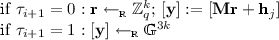
  • – $\mathsf {EncO}(\tau )$ computes $(K,C) \leftarrow _{\textsc {r}}{\mathsf {Enc_{KEM}}}(\mathsf {pk},\tau )$, sets $K_0 :=K$ and $K_1 \leftarrow _{\textsc {r}}\mathcal {K}$. If $\tau \notin \mathcal {T}_\mathsf {dec}\cup \mathcal {T}_\mathsf {enc}$, it returns $(C,K_b)$, and sets $\mathcal {T}_\mathsf {enc}:= \mathcal {T}_\mathsf {enc}\cup \{\tau \}$; otherwise it returns $\bot$.

  We say ${\mathsf {KEM}}$ is ${\mathrm {IND\text{- }PCA}}$ secure if for all $\mathsf {PPT}$ adversaries $\mathcal {A}$, the advantage $\mathbf {Adv}^{\mathsf {ind\text{- }pca}}_{{\mathsf {KEM}}}(\mathcal {A})$ is a negligible function of $\lambda$.

2.7 Authenticated Encryption

Definition 7

(AE [17]). An authenticated symmetric encryption (AE) with message-space $\mathcal {M}$ and key-space $\mathcal {K}$ consists of two polynomial-time deterministic algorithms $({\mathsf {Enc_{AE}}},{\mathsf {Dec_{AE}}})$:

• The encryption algorithm ${\mathsf {Enc_{AE}}}(K,M)$ generates C, encryption of the message M with the secret key K.

• The decryption algorithm ${\mathsf {Dec_{AE}}}(K,C)$, returns a message M or $\bot$.

We require that the algorithms satisfy the following properties:

• Perfect Correctness. For all $\lambda$, for all $K \in \mathcal {K}$ and $M\in \mathcal {M}$, we have

  $$\begin{aligned} {\mathsf {Dec_{AE}}}(K,{\mathsf {Enc_{AE}}}(K,M))=M. \end{aligned}$$

• One-Time Privacy and Authenticity. For any PPT adversary $\mathcal {A}$,

  $$\begin{aligned}&\mathbf {Adv}^{\mathsf {ae\text{- }ot}}_{\mathsf {AE}}(\mathcal {A}) \\&:=\left| \Pr \left[ b' = b \left| \begin{array}{l} K \leftarrow _{\textsc {r}}\mathcal {K}; b \leftarrow _{\textsc {r}}\{0,1\}\\ b' \leftarrow _{\textsc {r}}\mathcal {A}^{\mathsf {ot\text{- }EncO}(\cdot ,\cdot ),\mathsf {ot\text{- }DecO}(\cdot )}(1^\lambda ,\mathcal {K}) \end{array} \right. \right] - 1/2 \right| \end{aligned}$$

  is negligible, where $\mathsf {ot\text{- }EncO}(M_0,M_1)$, on input two messages $M_0$ and $M_1$ of the same length, ${\mathsf {Enc_{AE}}}(K,M_b)$, and $\mathsf {ot\text{- }DecO}(\phi )$ returns ${\mathsf {Dec_{AE}}}(K,\phi )$ if $b=0$, $\bot$ otherwise. $\mathcal {A}$ is allowed at most one call to each oracle $\mathsf {ot\text{- }EncO}$ and $\mathsf {ot\text{- }DecO}$, and the query to $\mathsf {ot\text{- }DecO}$ must be different from the output of $\mathsf {ot\text{- }EncO}$. $\mathcal {A}$ is also given the description of the key-space $\mathcal {K}$ as input.

3 Multi-ciphertext PCA-secure KEM

In this section we describe a tag-based Key Encapsulation Mechanism ${\mathsf {KEM}}_{\mathsf {PCA}}$ that is ${\mathrm {IND\text{- }PCA}}$-secure (see Definition 6).

For simplicity, we use the matrix distribution $\mathcal {U}_{3k,k}$ in our scheme in Fig. 4, and prove it secure under the $\mathcal {U}_k$-$\mathsf {MDDH}$ Assumption ($\Leftrightarrow$ $\mathcal {U}_{3k,k}$-$\mathsf {MDDH}$ Assumption, by Lemma 1), which in turn admits a tight reduction to the standard k-$\mathsf {Lin}$ Assumption. However, using a matrix distribution $\mathcal {D}_{3k,k}$ with more compact representation yields a more efficient scheme, secure under the $\mathcal {D}_{3k,k}$-$\mathsf {MDDH}$ Assumption (see Remark 1).

3.1 Our Construction

Remark 1

(On the use of the $\mathcal {U}_k$-$\mathsf {MDDH}$ Assumption). In our scheme, we use a matrix distribution $\mathcal {U}_{3k,k}$ for the matrix $\mathbf {M}$, therefore proving security under the $\mathcal {U}_{3k,k}$-$\mathsf {MDDH}$ Assumption $\Leftrightarrow$ $\mathcal {U}_k$-$\mathsf {MDDH}$ Assumption (see Lemma 2). This is for simplicity of presentation. However, for efficiency, one may want to use an assumption with a more compact representation, such as the $\mathcal {CI}_{3k,k}$-$\mathsf {MDDH}$ Assumption [26] with representation size 2k instead of $3k^2$ for $\mathcal {U}_{3k,k}$.

Fig. 4.

${\mathsf {KEM}}_{\mathsf {PCA}}$, an ${\mathrm {IND\text{- }PCA}}$-secure KEM under the $\mathcal {U}_k$-$\mathsf {MDDH}$ Assumption, with tag-space $\mathcal {T}= \{0,1\}^\lambda$. Here, ${\mathsf {GGen}}$ is a prime-order group generator (see Sect. 2.3).

3.2 Security Proof

Theorem 1

The tag-based Key Encapsulation Mechanism ${\mathsf {KEM}}_{\mathsf {PCA}}$ defined in Fig. 4 has perfect correctness. Moreover, if the $\mathcal {U}_k$-$\mathsf {MDDH}$ Assumption holds in $\mathbb {G}$, ${\mathsf {KEM}}_{\mathsf {PCA}}$ is ${\mathrm {IND\text{- }PCA}}$ secure. Namely, for any adversary $\mathcal {A}$, there exists an adversary $\mathcal {B}$ such that $\mathbf {T}(\mathcal {B}) \approx \mathbf {T}(\mathcal {A}) + (Q_\mathsf {dec}+Q_\mathsf {enc})\cdot \mathsf {poly}(\lambda )$ and

$$\begin{aligned} \mathbf {Adv}^{\mathsf {ind\text{- }pca}}_{{\mathsf {KEM}}_{\mathsf {PCA}}}(\mathcal {A}) \le (4\lambda +1) \cdot \mathbf {Adv}^\mathrm {mddh}_{\mathcal {U}_{k},\mathsf {GGen}}(\mathcal {B}) + (Q_\mathsf {dec}+Q_\mathsf {enc})\cdot 2^{- \varOmega (\lambda )}, \end{aligned}$$

where $Q_\mathsf {enc}$, $Q_\mathsf {dec}$ are the number of times $\mathcal {A}$ queries $\mathsf {EncO}$, $\mathsf {DecO}$, respectively, and $\mathsf {poly}(\lambda )$ is independent of $\mathbf {T}(\mathcal {A})$.

Proof of Theorem  1 . Perfect correctness follows readily from the fact that for all $\mathbf {r}\in \mathbb {Z}_q^k$ and $C = \mathbf {r}^{\!\scriptscriptstyle {\top }}\mathbf {M}^{\!\scriptscriptstyle {\top }}$, for all $\mathbf {k}\in \mathbb {Z}_q^{3k}$:

$$\begin{aligned} \mathbf {r}^{\!\scriptscriptstyle {\top }}(\mathbf {M}^{\!\scriptscriptstyle {\top }}\mathbf {k}) = C\cdot \mathbf {k}. \end{aligned}$$

We now prove the ${\mathrm {IND\text{- }PCA}}$ security of ${\mathsf {KEM}}_{\mathsf {PCA}}$. We proceed via a series of games described in Figs. 6 and 7 and we use $\mathbf {Adv}_i$ to denote the advantage of $\mathcal {A}$ in game ${\mathrm {G}}_i$. We also give a high-level picture of the proof in Fig. 5, summarizing the sequence of games.

Lemma 4

( ${\mathrm {G}}_0$ to ${\mathrm {G}}_1$ ). There exists an adversary $\mathcal {B}_0$ such that $\mathbf {T}(\mathcal {B}_0) \approx \mathbf {T}(\mathcal {A}) + (Q_\mathsf {enc}+ Q_\mathsf {dec})\cdot \mathsf {poly}(\lambda )$ and

$$\begin{aligned} |\mathbf {Adv}_0 - \mathbf {Adv}_1| \le \mathbf {Adv}^\mathrm {mddh}_{\mathcal {U}_{k},\mathsf {GGen}}(\mathcal {B}_0) + \frac{1}{q-1}, \end{aligned}$$

where $Q_\mathsf {enc}$, $Q_\mathsf {dec}$ are the number of times $\mathcal {A}$ queries $\mathsf {EncO}$, $\mathsf {DecO}$, respectively, and $\mathsf {poly}(\lambda )$ is independent of $\mathbf {T}(\mathcal {A})$.

Here, we use the $\mathsf {MDDH}$ assumption to “tightly” switch the distribution of all the challenge ciphertexts.

Fig. 5.

Sequence of games for the proof of Theorem 1. Throughout, we have (i) $\mathbf {k}_\tau := \sum _{j=1}^\lambda \mathbf {k}_{j,\tau _j}$; (ii) $\mathsf {EncO}(\tau ) = ([\mathbf {y}],K_b)$ where $K_0 = [\mathbf {y}^{\!\scriptscriptstyle {\top }}\mathbf {k}'_\tau ]$ and $K_1 \leftarrow _{\textsc {r}}\mathbb {G}$; (iii) $\mathsf {DecO}(\tau ,[\mathbf {y}],\widehat{K})$ computes the encapsulation key $K:=[\mathbf {y}^{\!\scriptscriptstyle {\top }}\cdot \mathbf {k}'_\tau ]$. Here, $(\mathbf {M}_0^*,\mathbf {M}_1^*)$ is a basis for $\mathsf {span}(\mathbf {M}^\perp )$, so that $\mathbf {M}_1^\perp \mathbf {M}_0^* = \mathbf {M}_0^\perp \mathbf {M}_1^* = \mathbf {0}$, and we write $\mathbf {M}^\perp \mathsf {RF}_i(\tau _{|i}) := \mathbf {M}_0^* \mathsf {RF}^{(0)}_i(\tau _{|i}) + \mathbf {M}_0^* \mathsf {RF}^{(1)}_i(\tau _{|i})$. The second column shows which set $\mathbf {y}$ is uniformly picked from by $\mathsf {EncO}$, the third column shows the value of $\mathbf {k}'_\tau$ used by both $\mathsf {EncO}$ and $\mathsf {DecO}$.

Fig. 6.

Games ${\mathrm {G}}_0,{\mathrm {G}}_1,{\mathrm {G}}_{2.i} \ (\text{ for } 1 \le i \le \lambda )$ for the proof of multi-ciphertext PCA security of ${\mathsf {KEM}}_{\mathsf {PCA}}$ in Fig. 4. For all $0 \le i \le \lambda$, $\mathsf {RF}_i: \{0,1\}^i \rightarrow \mathbb {Z}_q^{2k}$ is a random function, and for all $\tau \in \mathcal {T}$, $\tau _{|i}$ denotes the i-bit prefix of $\tau$. In each procedure, the components inside a solid (dotted) frame are only present in the games marked by a solid (dotted) frame.

Proof of Lemma  4 . To go from ${\mathrm {G}}_{0}$ to ${\mathrm {G}}_{1}$, we switch the distribution of the vectors $[\mathbf {y}]$ sampled by $\mathsf {EncO}$, using the $Q_\mathsf {enc}$-fold $\mathcal {U}_{3k,k}$-$\mathsf {MDDH}$ Assumption on $[\mathbf {M}]$ (see Definition 4 and Lemma 3).

We build an adversary $\mathcal {B}'_0$ against the $Q_\mathsf {enc}$-fold $\mathcal {U}_{3k,k}$-$\mathsf {MDDH}$ Assumption, such that $\mathbf {T}(\mathcal {B}'_0) \approx \mathbf {T}(\mathcal {A}) + (Q_\mathsf {enc}+ Q_\mathsf {dec})\cdot \mathsf {poly}(\lambda )$ with $\mathsf {poly}(\lambda )$ independent of $\mathbf {T}(\mathcal {A})$, and

$$\begin{aligned} |\mathbf {Adv}_{0} - \mathbf {Adv}_{1}| \le \mathbf {Adv}^\mathrm {Q_\mathsf {enc}\text{- }mddh}_{\mathcal {U}_{3k,k},\mathsf {GGen}}(\mathcal {B}'_0). \end{aligned}$$

This implies the lemma by Lemma 3 (self-reducibility of $\mathcal {U}_{3k,k}$-$\mathsf {MDDH}$), and Lemma 1 ($\mathcal {U}_{3k,k}$-$\mathsf {MDDH}\Leftrightarrow \mathcal {U}_k$-$\mathsf {MDDH}$).

Upon receiving a challenge $({\mathcal G},[\mathbf {M}]\in \mathbb {G}^{3k \times k},[\mathbf {H}] := [\mathbf {h}_1 | \ldots | \mathbf {h}_{Q_\mathsf {enc}}] \in \mathbb {G}^{3k \times Q_\mathsf {enc}})$ for the $Q_\mathsf {enc}$-fold $\mathcal {U}_{3k,k}$-$\mathsf {MDDH}$ Assumption, $\mathcal {B}'_0$ picks $b \leftarrow _{\textsc {r}}\{0,1\}$, $\mathbf {k}_{1,0}, \ldots , \mathbf {k}_{\lambda ,1} \leftarrow _{\textsc {r}}\mathbb {Z}_q^{3k}$, and simulates $\mathsf {Setup}$, $\mathsf {DecO}$ as described in Fig. 6. To simulate $\mathsf {EncO}$ on its j’th query, for $j=1,\ldots ,Q_\mathsf {enc}$, $\mathcal {B}'_0$ sets $[\mathbf {y}] := [\mathbf {h}_j]$, and computes $K_b$ as described in Fig. 6.    $\square$

Lemma 5

( ${\mathrm {G}}_1$ to ${\mathrm {G}}_{2.0}$ ).   $|\mathbf {Adv}_1 - \mathbf {Adv}_{2.0}|=0.$

Proof of Lemma  5 . We show that the two games are statistically equivalent. To go from ${\mathrm {G}}_1$ to ${\mathrm {G}}_{2.0}$, we change the distribution of $\mathbf {k}_{1,\beta } \leftarrow _{\textsc {r}}\mathbb {Z}_q^{3k}$ for $\beta =0,1$, to $\mathbf {k}_{1,\beta }+\mathbf {M}^\bot \mathsf {RF}_0(\varepsilon )$, where $\mathbf {k}_{1,\beta } \leftarrow _{\textsc {r}}\mathbb {Z}_q^{3k}$, $\mathsf {RF}_0(\varepsilon ) \leftarrow _{\textsc {r}}\mathbb {Z}^{2k}_q$, and $\mathbf {M}^\bot \leftarrow _{\textsc {r}}\mathcal {U}_{3k , 2k}$ such that $\mathbf {M}^{\!\scriptscriptstyle {\top }}\mathbf {M}^\bot = \mathbf {0}$. Note that the extra term $\mathbf {M}^\bot \mathsf {RF}_0(\varepsilon )$ does not appear in $\mathsf {pk}$, since $\mathbf {M}^{\!\scriptscriptstyle {\top }}(\mathbf {k}_{1,\beta } + \mathbf {M}^\bot \mathsf {RF}_0(\varepsilon )) = \mathbf {M}^{\!\scriptscriptstyle {\top }}\mathbf {k}_{1,\beta }$.    $\square$

Lemma 6

( ${\mathrm {G}}_{2.i}$ to ${\mathrm {G}}_{2.i+1}$ ). For all $0 \le i \le \lambda -1$, there exists an adversary $\mathcal {B}_{2.i}$ such that $\mathbf {T}(\mathcal {B}_{2.i}) \approx \mathbf {T}(\mathcal {A}) + (Q_\mathsf {enc}+ Q_\mathsf {dec})\cdot \mathsf {poly}(\lambda )$ and

$$\begin{aligned} | \mathbf {Adv}_{2.i} - \mathbf {Adv}_{2.i+1} | \le 4 \cdot \mathbf {Adv}^\mathrm {mddh}_{\mathcal {U}_{k},\mathsf {GGen}}(\mathcal {B}_{2.i})+ \frac{4Q_\mathsf {dec}+2k}{q} + \frac{4}{q-1}, \end{aligned}$$

where $Q_\mathsf {enc}$, $Q_\mathsf {dec}$ are the number of times $\mathcal {A}$ queries $\mathsf {EncO}$, $\mathsf {DecO}$, respectively, and $\mathsf {poly}(\lambda )$ is independent of $\mathbf {T}(\mathcal {A})$.

Proof of Lemma  6 . To go from ${\mathrm {G}}_{2.i}$ to ${\mathrm {G}}_{2.i+1}$, we introduce intermediate games ${\mathrm {G}}_{2.i.1}$, ${\mathrm {G}}_{2.i.2}$ and ${\mathrm {G}}_{2.i.3}$, defined in Fig. 7. We prove that these games are indistinguishable in Lemmas 7, 8, 9, and 10.

Fig. 7.

Games ${\mathrm {G}}_{2.i}$ (for $0 \le i \le \lambda$),${\mathrm {G}}_{2.i.1}$, ${\mathrm {G}}_{2.i.2}$ and ${\mathrm {G}}_{2.i.3}$ (for $0 \le i \le \lambda -1$) for the proof of Lemma 6. For all $0 \le i \le \lambda$, $\mathsf {RF}_i:\{0,1\}^i \rightarrow \mathbb {Z}^{2k}_q$, $\mathsf {RF}_i^{(0)}$, $\mathsf {RF}_i^{(1)} : \{0,1\}^{i} \rightarrow \mathbb {Z}_q^{k}$ are random functions, and for all $\tau \in \mathcal {T}$, we denote by $\tau _{|i}$ the i-bit prefix of $\tau$. In each procedure, the components inside a solid (dotted, gray) frame are only present in the games marked by a solid (dotted, gray) frame.

Lemma 7

( ${\mathrm {G}}_{2.i}$ to ${\mathrm {G}}_{2.i.1}$ ). For all $0 \le i \le \lambda -1$, there exists an adversary $\mathcal {B}_{2.i.0}$ such that $\mathbf {T}(\mathcal {B}_{2.i.0}) \approx \mathbf {T}(\mathcal {A})+(Q_\mathsf {enc}+ Q_\mathsf {dec})\cdot \mathsf {poly}(\lambda )$ and

$$\begin{aligned} | \mathbf {Adv}_{2.i} - \mathbf {Adv}_{2.i.1} | \le 2 \cdot \mathbf {Adv}^\mathrm {mddh}_{\mathcal {U}_{k},\mathsf {GGen}}(\mathcal {B}_{2.i.0})+ \frac{2}{q-1}, \end{aligned}$$

where $Q_\mathsf {enc}$, $Q_\mathsf {dec}$ are the number of times $\mathcal {A}$ queries $\mathsf {EncO}$, $\mathsf {DecO}$, respectively, and $\mathsf {poly}(\lambda )$ is independent of $\mathbf {T}(\mathcal {A})$.

Here, we use the $\mathsf {MDDH}$ Assumption to “tightly” switch the distribution of all the challenge ciphertexts. We proceed in two steps, first, by changing the distribution of all the ciphertexts with a tag $\tau$ such that $\tau _{i+1}=0$, and then, for those with a tag $\tau$ such that $\tau _{i+1}=1$. We use the $\mathsf {MDDH}$ Assumption with respect to an independent matrix for each step.

Proof of Lemma  7 . To go from ${\mathrm {G}}_{2.i}$ to ${\mathrm {G}}_{2.i.1}$, we switch the distribution of the vectors $[\mathbf {y}]$ sampled by $\mathsf {EncO}$, using the $Q_\mathsf {enc}$-fold $\mathcal {U}_{3k,k}$-$\mathsf {MDDH}$ Assumption.

We introduce an intermediate game ${\mathrm {G}}_{2.i.0}$ where $\mathsf {EncO}(\tau )$ is computed as in ${\mathrm {G}}_{2.i.1}$ if $\tau _{i+1}=0$, and as in ${\mathrm {G}}_{2.i}$ if $\tau _{i+1}=1$. $\mathsf {Setup}$, $\mathsf {DecO}$ are as in ${\mathrm {G}}_{2.i.1}$. We build adversaries $\mathcal {B}'_{2.i.0}$ and $\mathcal {B}''_{2.i.0}$ such that $\mathbf {T}(\mathcal {B}'_{2.i.0}) \approx \mathbf {T}(\mathcal {B}''_{2.i.0}) \approx \mathbf {T}(\mathcal {A})+(Q_\mathsf {enc}+ Q_\mathsf {dec})\cdot \mathsf {poly}(\lambda )$ with $\mathsf {poly}(\lambda )$ independent of $\mathbf {T}(\mathcal {A})$, and

• Claim 1: $|\mathbf {Adv}_{2.i} - \mathbf {Adv}_{2.i.0}| \le \mathbf {Adv}^\mathrm {Q_\mathsf {enc}\text{- }mddh}_{\mathcal {U}_{3,k},\mathsf {GGen}}(\mathcal {B}'_{2.i.0})$.

• Claim 2: $|\mathbf {Adv}_{2.i.0} - \mathbf {Adv}_{2.i.1}| \le \mathbf {Adv}^\mathrm {Q_\mathsf {enc}\text{- }mddh}_{\mathcal {U}_{3k,k},\mathsf {GGen}}(\mathcal {B}''_{2.i.0})$.

This implies the lemma by Lemma 3 (self-reducibility of $\mathcal {U}_{3k,k}$-$\mathsf {MDDH}$), and Lemma 1 ($\mathcal {U}_{3k,k}$-$\mathsf {MDDH}\Leftrightarrow \mathcal {U}_k$-$\mathsf {MDDH}$).

Let us prove Claim 1. Upon receiving a challenge $({\mathcal G},[\mathbf {M}_0]\in \mathbb {G}^{3k \times k},[\mathbf {H}] := [\mathbf {h}_1 | \ldots | \mathbf {h}_{Q_\mathsf {enc}}] \in \mathbb {G}^{3k \times Q_\mathsf {enc}})$ for the $Q_\mathsf {enc}$-fold $\mathcal {U}_{3k,k}$-$\mathsf {MDDH}$ Assumption with respect to $\mathbf {M}_0 \leftarrow _{\textsc {r}}\mathcal {U}_{3k,k}$, $\mathcal {B}'_{2.i.0}$ does as follows:

• $\mathsf {Setup}$: $\mathcal {B}'_{2.i.0}$ picks $\mathbf {M}\leftarrow _{\textsc {r}}\mathcal {U}_{3k,k}$, $\mathbf {k}_{1,0}, \ldots , \mathbf {k}_{\lambda ,1} \leftarrow _{\textsc {r}}\mathbb {Z}_q^{3k}$, and computes $\mathsf {pk}$ as described in Fig. 7. For each $\tau$ queried to $\mathsf {EncO}$ or $\mathsf {DecO}$, it computes on the fly $\mathsf {RF}_i(\tau _{|i})$ and $\mathbf {k}'_\tau := \mathbf {k}_\tau + \mathbf {M}^\bot \mathsf {RF}_i(\tau _{|i})$, where $\mathbf {k}_\tau := \sum _{j=1}^\lambda \mathbf {k}_{j,\tau _j}$, $\mathsf {RF}_i : \{0,1\}^i \rightarrow \mathbb {Z}_q^{2k}$ is a random function, and $\tau _{|i}$ denotes the i-bit prefix of $\tau$ (see Fig. 7). Note that $\mathcal {B}'_{2.i.0}$ can compute efficiently $\mathbf {M}^\bot$ from $\mathbf {M}$.

• $\mathsf {EncO}$: To simulate the oracle $\mathsf {EncO}(\tau )$ on its j’th query, for $j=1,\ldots ,Q_\mathsf {enc}$, $\mathcal {B}'_{2.i.0}$ computes $[\mathbf {y}]$ as follows:

  

  This way, $\mathcal {B}'_{2.i.0}$ simulates $\mathsf {EncO}$ as in ${\mathrm {G}}_{2.i.0}$ when $[\mathbf {h}_j] := [\mathbf {M}_0 \mathbf {r}_0]$ with $\mathbf {r}_0 \leftarrow _{\textsc {r}}\mathbb {Z}_q^{k}$, and as in ${\mathrm {G}}_{2.i}$ when $[\mathbf {h}_j] \leftarrow _{\textsc {r}}\mathbb {G}^{3k}$.

• $\mathsf {DecO}$: Finally, $\mathcal {B}'_{2.i.0}$ simulates $\mathsf {DecO}$ as described in Fig. 7.

Therefore, $|\mathbf {Adv}_{2.i} - \mathbf {Adv}_{2.i.0}| \le \mathbf {Adv}^\mathrm {Q_\mathsf {enc}\text{- }mddh}_{\mathcal {U}_{3k,k},\mathsf {GGen}}(\mathcal {B}'_{2.i.0})$.

To prove Claim 2, we build an adversary $\mathcal {B}''_{2.i.0}$ against the $Q_\mathsf {enc}$-fold $\mathcal {U}_{3k,k}$-$\mathsf {MDDH}$ Assumption with respect to a matrix $\mathbf {M}_1 \leftarrow _{\textsc {r}}\mathcal {U}_{3k,k}$, independent from $\mathbf {M}_0$, similarly than $\mathcal {B}'_{2.i.0}$.    $\square$

Lemma 8

( ${\mathrm {G}}_{2.i.1}$ to ${\mathrm {G}}_{2.i.2}$ ). For all $0 \le i \le \lambda -1$,

$$\begin{aligned} | \mathbf {Adv}_{2.i.1} - \mathbf {Adv}_{2.i.2} | \le \frac{2Q_\mathsf {dec}+2k}{q} , \end{aligned}$$

where $Q_\mathsf {dec}$ is the number of times $\mathcal {A}$ queries $\mathsf {DecO}$.

Here, we use a variant of the Cramer-Shoup information-theoretic argument to move from $\mathsf {RF}_i$ to $\mathsf {RF}_{i+1}$, thereby increasing the entropy of $\mathbf {k}'_\tau$ computed by $\mathsf {Setup}$. For the sake of readability, we proceed in two steps: in Lemma 8, we move from $\mathsf {RF}_i$ to an hybrid between $\mathsf {RF}_i$ and $\mathsf {RF}_{i+1}$, and in Lemma 9, we move to $\mathsf {RF}_{i+1}$.

Proof of Lemma  8 . In ${\mathrm {G}}_{2.i.2}$, we decompose $\mathsf {span}(\mathbf {M}^\bot )$ into two subspaces $\mathsf {span}(\mathbf {M}_0^*)$ and $\mathsf {span}(\mathbf {M}_1^*)$, and we increase the entropy of the components of $\mathbf {k}'_\tau$ which lie in $\mathsf {span}(\mathbf {M}_0^*)$. To argue that ${\mathrm {G}}_{2.i.1}$ and ${\mathrm {G}}_{2.i.2}$ are statistically close, we use a Cramer-Shoup argument [11].

Let us first explain how the matrices $\mathbf {M}_0^*$ and $\mathbf {M}_1^*$ are sampled. Note that with probability at least $1-\frac{2k}{q}$ over the random coins of $\mathsf {Setup}$, $(\mathbf {M}\Vert \mathbf {M}_0 \Vert \mathbf {M}_1)$ forms a basis of $\mathbb {Z}_q^{3k}$. Therefore, we have

$$\begin{aligned} \mathsf {span}(\mathbf {M}^\bot ) = \mathsf {Ker}(\mathbf {M}^{\!\scriptscriptstyle {\top }}) = \mathsf {Ker}\big ((\mathbf {M}\Vert \mathbf {M}_1)^{\!\scriptscriptstyle {\top }}\big ) \oplus \mathsf {Ker}\big ((\mathbf {M}\Vert \mathbf {M}_0)^{\!\scriptscriptstyle {\top }}\big ). \end{aligned}$$

We pick uniformly $\mathbf {M}_0^*$ and $\mathbf {M}_1^*$ in $\mathbb {Z}_q^{3k \times k}$ that generate $\mathsf {Ker}\big ((\mathbf {M}\Vert \mathbf {M}_1)^{\!\scriptscriptstyle {\top }}\big )$ and $\mathsf {Ker}\big ((\mathbf {M}\Vert \mathbf {M}_0)^{\!\scriptscriptstyle {\top }}\big )$, respectively (see Fig. 1). This way, for all $\tau \in \{0,1\}^\lambda$, we can write

$$\begin{aligned} \mathbf {M}^\bot \mathsf {RF}_{i}(\tau _{|i}) := \mathbf {M}_0^* \mathsf {RF}^{(0)}_{i}(\tau _{|i}) + \mathbf {M}_1^* \mathsf {RF}^{(1)}_{i}(\tau _{|i}), \end{aligned}$$

where $\mathsf {RF}^{(0)}_i$, $\mathsf {RF}^{(1)}_i: \{0,1\}^i \rightarrow \mathbb {Z}_q^k$ are independent random functions.

We define $\mathsf {RF}^{(0)}_{i+1}: \{0,1\}^{i+1} \rightarrow \mathbb {Z}_q^{k}$ as follows:

$$\begin{aligned} \mathsf {RF}^{(0)}_{i+1}(\tau _{|i+1}) := {\left\{ \begin{array}{ll} \mathsf {RF}^{(0)}_i(\tau _{|i}) &{} \text{ if } \tau _{i+1} = 0 \\ \mathsf {RF}^{(0)}_{i}(\tau _{|i}) + {\mathsf {RF}'}^{(0)}_{i}(\tau _{|i}) &{} \text{ if } \tau _{i+1} = 1 \end{array}\right. } \end{aligned}$$

where ${\mathsf {RF}'}^{(0)}_{i}: \{0,1\}^{i} \rightarrow \mathbb {Z}_q^{k}$ is a random function independent from $\mathsf {RF}^{(0)}_i$. This way, $\mathsf {RF}^{(0)}_{i+1}$ is a random function.

We show that the outputs of $\mathsf {EncO}$ and $\mathsf {DecO}$ are statistically close in ${\mathrm {G}}_{2.i.1}$ and ${\mathrm {G}}_{2.i.2}$. We decompose the proof in two cases (delimited with $\blacksquare$): the queries with a tag $\tau \in \{0,1\}^\lambda$ such that $\tau _{i+1}=0$, and the queries with a tag $\tau$ such that $\tau _{i+1}=1$.

Queries with $\tau _{i+1}=0$ :

The only difference between ${\mathrm {G}}_{2.i.1}$ and ${\mathrm {G}}_{2.i.2}$ is that $\mathsf {Setup}$ computes $\mathbf {k}'_\tau$ using the random function $\mathsf {RF}^{(0)}_{i}$ in ${\mathrm {G}}_{2.i.1}$, whereas it uses the random function $\mathsf {RF}^{(0)}_{i+1}$ in ${\mathrm {G}}_{2.i.2}$ (see Fig. 7). Therefore, by definition of $\mathsf {RF}_{i+1}^{(0)}$, for all $\tau \in \{0,1\}^\lambda$ such that $\tau _{i+1}=0$, $\mathbf {k}'_\tau$ is the same in ${\mathrm {G}}_{2.i.1}$ and ${\mathrm {G}}_{2.i.2}$, and the outputs of $\mathsf {EncO}$ and $\mathsf {DecO}$ are identically distributed. $\blacksquare$

Queries with $\tau _{i+1}=1$ :

Observe that for all $\mathbf {y}\in \mathsf {span}(\mathbf {M},\mathbf {M}_1)$ and all $\tau \in \{0,1\}^\lambda$ such that $\tau _{i+1}=1$,

$$\begin{aligned}&\overbrace{\mathbf {y}^{\!\scriptscriptstyle {\top }}\Big (\mathbf {k}_\tau + \mathbf {M}_0^* \mathsf {RF}^{(0)}_i(\tau _{|i}) + \mathbf {M}_1^* \mathsf {RF}^{(1)}_i(\tau _{|i}) + \boxed {\mathbf {M}_0^*{\mathsf {RF}'}^{(0)}_{i}(\tau _{|i})}\Big )}^{{\mathrm {G}}_{2.i.2}} \\&= \mathbf {y}^{\!\scriptscriptstyle {\top }}\Big (\mathbf {k}_\tau + \mathbf {M}_0^* \mathsf {RF}^{(0)}_i(\tau _{|i}) + \mathbf {M}_1^* \mathsf {RF}^{(1)}_i(\tau _{|i})\Big ) + \underbrace{\boxed {\mathbf {y}^{\!\scriptscriptstyle {\top }}\mathbf {M}_0^*{\mathsf {RF}'}^{(0)}_{i}(\tau _{|i})}}_{=0} \\&= \overbrace{\mathbf {y}^{\!\scriptscriptstyle {\top }}\cdot \Big (\mathbf {k}_\tau + \mathbf {M}_0^* \mathsf {RF}^{(0)}_i(\tau _{|i}) + \mathbf {M}_1^* \mathsf {RF}^{(1)}_i(\tau _{|i})\Big )}^{{\mathrm {G}}_{2.i.1}} \end{aligned}$$

where the second equality uses the fact that $\mathbf {M}^{\!\scriptscriptstyle {\top }}\mathbf {M}_0^* = \mathbf {M}_1^{\!\scriptscriptstyle {\top }}\mathbf {M}_0^* = \mathbf {0}$ and thus $\mathbf {y}^{\!\scriptscriptstyle {\top }}\mathbf {M}_0^* = \mathbf {0}$.

This means that:

• the output of $\mathsf {EncO}$ on any input $\tau$ such that $\tau _{i+1}=1$ is identically distributed in ${\mathrm {G}}_{2.i.1}$ and ${\mathrm {G}}_{2.i.2}$;

• the output of $\mathsf {DecO}$ on any input $(\tau , [\mathbf {y}], \widehat{K})$ where $\tau _{i+1}=1$, and $\mathbf {y}\in \mathsf {span}(\mathbf {M},\mathbf {M}_1)$ is the same in ${\mathrm {G}}_{2.i.1}$ and ${\mathrm {G}}_{2.i.2}$.

Henceforth, we focus on the ill-formed queries to $\mathsf {DecO}$, namely those corresponding to $\tau _{i+1}=1$, and $\mathbf {y}\notin \mathsf {span}(\mathbf {M},\mathbf {M}_1)$. We introduce intermediate games ${\mathrm {G}}_{2.i.1.j}$, and ${\mathrm {G}}'_{2.i.1.j}$ for $j=0,\ldots ,Q_\mathsf {dec}$, defined as follows:

• ${\mathrm {G}}_{2.i.1.j}$: $\mathsf {DecO}$ is as in ${\mathrm {G}}_{2.i.1}$ except that for the first j times it is queried, it outputs 0 to any ill-formed query. $\mathsf {EncO}$ is as in ${\mathrm {G}}_{2.i.2}$.

• ${\mathrm {G}}'_{2.i.1.j}$: $\mathsf {DecO}$ as in ${\mathrm {G}}_{2.i.2}$ except that for the first j times it is queried, it outputs 0 to any ill-formed query. $\mathsf {EncO}$ is as in ${\mathrm {G}}_{2.i.2}$.

We show that:

$$\begin{aligned}&{\mathrm {G}}_{2.i.1} \equiv {\mathrm {G}}_{2.i.1.0} \approx _s {\mathrm {G}}_{2.i.1.1} \approx _s \ldots \approx _s {\mathrm {G}}_{2.i.1.Q_\mathsf {dec}} \equiv {\mathrm {G}}'_{2.i.1.Q_\mathsf {dec}}\\&{\mathrm {G}}'_{2.i.1.Q_\mathsf {dec}} \approx _s {\mathrm {G}}'_{2.i.1.Q_\mathsf {dec}-1} \approx _s \ldots \approx _s {\mathrm {G}}'_{2.i.1.0} \equiv {\mathrm {G}}_{2.i.2} \end{aligned}$$

where we denote statistical closeness with $\approx _s$ and statistical equality with $\equiv$.

It suffices to show that for all $j=0,\ldots ,Q_\mathsf {dec}-1$:

• Claim 1: in ${\mathrm {G}}_{2.i.1.j}$, if the $j+1$-st query is ill-formed, then $\mathsf {DecO}$ outputs 0 with overwhelming probability $1-1/q$ (this implies ${\mathrm {G}}_{2.i.1.j} \approx _s {\mathrm {G}}_{2.i.1.j+1}$, with statistical difference 1 / q);

• Claim 2: in ${\mathrm {G}}'_{2.i.1.j}$, if the $j+1$-st query is ill-formed, then $\mathsf {DecO}$ outputs 0 with overwhelming probability $1-1/q$ (this implies ${\mathrm {G}}'_{2.i.1.j} \approx _s {\mathrm {G}}'_{2.i.1.j+1}$, with statistical difference 1 / q)

where the probabilities are taken over the random coins of $\mathsf {Setup}$.

Let us prove Claim 1. Recall that in ${\mathrm {G}}_{2.i.1.j}$, on its $j+1$-st query, $\mathsf {DecO}(\tau ,[\mathbf {y}],\widehat{K})$ computes $K := \left[ \mathbf {y}^{\!\scriptscriptstyle {\top }}\mathbf {k}'_\tau \right]$, where $\mathbf {k}'_\tau := \big (\mathbf {k}_\tau + \mathbf {M}_0^* \mathsf {RF}^{(0)}_i(\tau _{|i}) + \mathbf {M}_1^* \mathsf {RF}^{(1)}_i(\tau _{|i})\big )$ (see Fig. 7). We prove that if $(\tau ,[\mathbf {y}],\widehat{K})$ is ill-formed, then K is completely hidden from $\mathcal {A}$, up to its $j+1$-st query to $\mathsf {DecO}$. The reason is that the vector $\mathbf {k}_{i+1,1}$ in $\mathsf {sk}$ contains some entropy that is hidden from $\mathcal {A}$. This entropy is “released” on the $j+1$-st query to $\mathsf {DecO}$ if it is ill-formed. More formally, we use the fact that the vector $\mathbf {k}_{i+1,1} \leftarrow _{\textsc {r}}\mathbb {Z}_q^{3k}$ is identically distributed as $\mathbf {k}_{i+1,1} + \mathbf {M}_0^* \mathbf {w}$, where $\mathbf {k}_{i+1,1} \leftarrow _{\textsc {r}}\mathbb {Z}_q^{3k}$, and $\mathbf {w}\leftarrow _{\textsc {r}}\mathbb {Z}_q^{k}$. We show that $\mathbf {w}$ is completely hidden from $\mathcal {A}$, up to its $j+1$-st query to $\mathsf {DecO}$.

• The public key $\mathsf {pk}$ does not leak any information about $\mathbf {w}$, since

  $$\begin{aligned} \mathbf {M}^{\!\scriptscriptstyle {\top }}(\mathbf {k}_{i+1,1} + \boxed {\mathbf {M}_0^* \mathbf {w}}) = \mathbf {M}^{\!\scriptscriptstyle {\top }}\mathbf {k}_{i+1,1}. \end{aligned}$$

  This is because $\mathbf {M}^{\!\scriptscriptstyle {\top }}\mathbf {M}_0^* = \mathbf {0}$.

• The outputs of $\mathsf {EncO}$ also hide $\mathbf {w}$.

  • For $\tau$ such that $\tau _{i+1}=0$, $\mathbf {k}'_\tau$ is independent of $\mathbf {k}_{i+1,1}$, and therefore, so does $\mathsf {EncO}(\tau )$.

  • For $\tau$ such that $\tau _{i+1}=1$, and for any $\mathbf {y}\in \mathsf {span}(\mathbf {M},\mathbf {M}_1)$, we have:

    $$\begin{aligned} \mathbf {y}^{\!\scriptscriptstyle {\top }}(\mathbf {k}'_\tau + \boxed {\mathbf {M}_0^*\mathbf {w}}) = \mathbf {y}^{\!\scriptscriptstyle {\top }}\mathbf {k}'_\tau \end{aligned}$$

    (2)

    since $\mathbf {M}^{\!\scriptscriptstyle {\top }}\mathbf {M}_0^* = \mathbf {M}_1^{\!\scriptscriptstyle {\top }}\mathbf {M}_0^* = \mathbf {0}$, which implies $\mathbf {y}^{\!\scriptscriptstyle {\top }}\mathbf {M}_0^* = \mathbf {0}$.

• The first j outputs of $\mathsf {DecO}$ also hide $\mathbf {w}$.

  • For $\tau$ such that $\tau _{i+1}=0$, $\mathbf {k}'_\tau$ is independent of $\mathbf {k}_{i+1,1}$, and therefore, so does $\mathsf {DecO}([\mathbf {y}],\tau ,\widehat{K})$.

  • For $\tau$ such that $\tau _{i+1}=1$ and $\mathbf {y}\in \mathsf {span}(\mathbf {M},\mathbf {M}_1)$, the fact that $\mathsf {DecO}(\tau ,[\mathbf {y}],\widehat{K})$ is independent of $\mathbf {w}$ follows readily from Equation (2).

  • For $\tau$ such that $\tau _{i+1}=1$ and $\mathbf {y}\notin \mathsf {span}(\mathbf {M},\mathbf {M}_1)$, that is, for an ill-formed query, $\mathsf {DecO}$ outputs 0, independently of $\mathbf {w}$, by definition of ${\mathrm {G}}_{2.i.1.j}$.

This proves that $\mathbf {w}$ is uniformly random from $\mathcal {A}$’s viewpoint.

Finally, because the $j+1$-st query $(\tau ,[\mathbf {y}],\widehat{K})$ is ill-formed, we have $\tau _{i+1}=1$, and $\mathbf {y}\notin \mathsf {span}(\mathbf {M},\mathbf {M}_1)$, which implies that $\mathbf {y}^{\!\scriptscriptstyle {\top }}\mathbf {M}_0^* \ne \mathbf {0}$. Therefore, the value

$$\begin{aligned} K = [\mathbf {y}^{\!\scriptscriptstyle {\top }}(\mathbf {k}'_\tau + \mathbf {M}_0^* \mathbf {w})] = [\mathbf {y}^{\!\scriptscriptstyle {\top }}\mathbf {k}_\tau ' + \underbrace{\mathbf {y}^{\!\scriptscriptstyle {\top }}\mathbf {M}_0^*}_{\ne \mathbf {0}} \mathbf {w}] \end{aligned}$$

computed by $\mathsf {DecO}$ is uniformly random over $\mathbb {G}$ from $\mathcal {A}$’s viewpoint. Thus, with probability $1-1/q$ over $K \leftarrow _{\textsc {r}}\mathbb {G}$, we have $\widehat{K} \ne K$, and $\mathsf {DecO}(\tau ,[\mathbf {y}],\widehat{K})=0$.

We prove Claim 2 similarly, arguing than in ${\mathrm {G}}'_{2.i.1.j}$, the value $K := \left[ \mathbf {y}^{\!\scriptscriptstyle {\top }}\mathbf {k}'_\tau \right]$, where $\mathbf {k}'_\tau := \big (\mathbf {k}_\tau + \mathbf {M}_0^* \mathsf {RF}^{(0)}_{i+1}(\tau _{|i+1}) + \mathbf {M}_1^* \mathsf {RF}^{(1)}_i(\tau _{|i})\big )$, computed by $\mathsf {DecO}(\tau ,[\mathbf {y}],\widehat{K})$ on its $j+1$-st query, is completely hidden from $\mathcal {A}$, up to its $j+1$-st query to $\mathsf {DecO}$, if $(\tau ,[\mathbf {y}],\widehat{K})$ is ill-formed. The argument goes exactly as for Claim 1. $\blacksquare$

Lemma 9

( ${\mathrm {G}}_{2.i.2}$ to ${\mathrm {G}}_{2.i.3}$ ). For all $0 \le i \le \lambda -1$,

$$\begin{aligned} | \mathbf {Adv}_{2.i.2} - \mathbf {Adv}_{2.i.3} | \le \frac{2Q_\mathsf {dec}}{q} , \end{aligned}$$

where $Q_\mathsf {dec}$ is the number of times $\mathcal {A}$ queries $\mathsf {DecO}$.

Proof of Lemma  9 . In ${\mathrm {G}}_{2.i.3}$, we use the same decomposition $\mathsf {span}(\mathbf {M}^\bot ) = \mathsf {span}(\mathbf {M}_0^*,\mathbf {M}_1^*)$ as that in ${\mathrm {G}}_{2.i.2}$. The entropy of the components of $\mathbf {k}'_\tau$ that lie in $\mathsf {span}(\mathbf {M}_1^*)$ increases from ${\mathrm {G}}_{2.i.2}$ to ${\mathrm {G}}_{2.i.3}$. To argue that these two games are statistically close, we use a Cramer-Shoup argument [11], exactly as for Lemma 8.

We define $\mathsf {RF}^{(1)}_{i+1} \{0,1\}^{i+1} \rightarrow \mathbb {Z}_q^{k}$ as follows:

$$\begin{aligned} \mathsf {RF}^{(1)}_{i+1}(\tau _{|i+1}) := {\left\{ \begin{array}{ll} \mathsf {RF}^{(1)}_i(\tau _{|i}) + {\mathsf {RF}'}^{(1)}_{i}(\tau _{|i}) &{} \text{ if } \tau _{i+1} = 0 \\ \mathsf {RF}^{(1)}_{i}(\tau _{|i}) &{} \text{ if } \tau _{i+1} = 1 \end{array}\right. } \end{aligned}$$

where ${\mathsf {RF}'}^{(1)}_{i}: \{0,1\}^{i} \rightarrow \mathbb {Z}_q^{k}$ is a random function independent from $\mathsf {RF}^{(1)}_i$. This way, $\mathsf {RF}^{(1)}_{i+1}$ is a random function.

We show that the outputs of $\mathsf {EncO}$ and $\mathsf {DecO}$ are statistically close in ${\mathrm {G}}_{2.i.1}$ and ${\mathrm {G}}_{2.i.2}$. We decompose the proof in two cases (delimited with $\blacksquare$): the queries with a tag $\tau \in \{0,1\}^\lambda$ such that $\tau _{i+1}=0$, and the queries with tag $\tau$ such that $\tau _{i+1}=1$.

Queries with $\tau _{i+1}=1$ :

The only difference between ${\mathrm {G}}_{2.i.2}$ and ${\mathrm {G}}_{2.i.3}$ is that $\mathsf {Setup}$ computes $\mathbf {k}'_\tau$ using the random function $\mathsf {RF}^{(1)}_{i}$ in ${\mathrm {G}}_{2.i.2}$, whereas it uses the random function $\mathsf {RF}^{(1)}_{i+1}$ in ${\mathrm {G}}_{2.i.3}$ (see Fig. 7). Therefore, by definition of $\mathsf {RF}_{i+1}^{(1)}$, for all $\tau \in \{0,1\}^\lambda$ such that $\tau _{i+1}=1$, $\mathbf {k}'_\tau$ is the same in ${\mathrm {G}}_{2.i.2}$ and ${\mathrm {G}}_{2.i.3}$, and the outputs of $\mathsf {EncO}$ and $\mathsf {DecO}$ are identically distributed. $\blacksquare$

Queries with $\tau _{i+1}=0$ :

Observe that for all $\mathbf {y}\in \mathsf {span}(\mathbf {M},\mathbf {M}_0)$ and all $\tau \in \{0,1\}^\lambda$ such that $\tau _{i+1}=0$,

$$\begin{aligned}&\overbrace{\mathbf {y}^{\!\scriptscriptstyle {\top }}\Big (\mathbf {k}_\tau + \mathbf {M}_0^* \mathsf {RF}^{(0)}_{i+1}(\tau _{|i+1}) + \mathbf {M}_1^* \mathsf {RF}^{(1)}_i(\tau _{|i}) + \boxed {\mathbf {M}_1^*{\mathsf {RF}'}^{(1)}_{i}(\tau _{|i})}\Big )}^{{\mathrm {G}}_{2.i.3}} \\&= \mathbf {y}^{\!\scriptscriptstyle {\top }}\Big (\mathbf {k}_\tau + \mathbf {M}_0^* \mathsf {RF}^{(0)}_{i+1}(\tau _{|i+1}) + \mathbf {M}_1^* \mathsf {RF}^{(1)}_i(\tau _{|i})\Big ) + \underbrace{\boxed {\mathbf {y}^{\!\scriptscriptstyle {\top }}\mathbf {M}_1^*{\mathsf {RF}'}^{(1)}_{i}(\tau _{|i})}}_{=0} \\&= \overbrace{\mathbf {y}^{\!\scriptscriptstyle {\top }}\cdot \Big (\mathbf {k}_\tau + \mathbf {M}_0^* \mathsf {RF}^{(0)}_{i+1}(\tau _{|i+1}) + \mathbf {M}_1^* \mathsf {RF}^{(1)}_i(\tau _{|i})\Big )}^{{\mathrm {G}}_{2.i.2}} \end{aligned}$$

where the second equality uses the fact $\mathbf {M}^{\!\scriptscriptstyle {\top }}\mathbf {M}_1^* = \mathbf {M}_0^{\!\scriptscriptstyle {\top }}\mathbf {M}_1^* = \mathbf {0}$, which implies $\mathbf {y}^{\!\scriptscriptstyle {\top }}\mathbf {M}_1^* = \mathbf {0}$.

This means that:

• the output of $\mathsf {EncO}$ on any input $\tau$ such that $\tau _{i+1}=0$ is identically distributed in ${\mathrm {G}}_{2.i.2}$ and ${\mathrm {G}}_{2.i.3}$;

• the output of $\mathsf {DecO}$ on any input $(\tau , [\mathbf {y}], \widehat{K})$ where $\tau _{i+1}=0$, and $\mathbf {y}\in \mathsf {span}(\mathbf {M},\mathbf {M}_0)$ is the same in ${\mathrm {G}}_{2.i.2}$ and ${\mathrm {G}}_{2.i.3}$.

Henceforth, we focus on the ill-formed queries to $\mathsf {DecO}$, namely those corresponding to $\tau _{i+1}=0$, and $\mathbf {y}\notin \mathsf {span}(\mathbf {M},\mathbf {M}_0)$. The rest of the proof goes similarly than the proof of Lemma 8. See the latter for further details.    $\square$

Lemma 10

( ${\mathrm {G}}_{2.i.3}$ to ${\mathrm {G}}_{2.i+1}$ ). For all $0 \le i \le \lambda -1$, there exists an adversary $\mathcal {B}_{2.i.3}$ such that $\mathbf {T}(\mathcal {B}_{2.i.3}) \approx \mathbf {T}(\mathcal {A}) + (Q_\mathsf {enc}+ Q_\mathsf {dec})\cdot \mathsf {poly}(\lambda )$ and

$$\begin{aligned} | \mathbf {Adv}_{2.i.3} - \mathbf {Adv}_{2.i+1} | \le 2\cdot \mathbf {Adv}^\mathrm {mddh}_{\mathcal {U}_{k},\mathsf {GGen}}(\mathcal {B}_{2.i.3}) + \frac{2}{q-1} \end{aligned}$$

where $Q_\mathsf {enc}$, $Q_\mathsf {dec}$ are the number of times $\mathcal {A}$ queries $\mathsf {EncO}$, $\mathsf {DecO}$, respectively, and $\mathsf {poly}(\lambda )$ is independent of $\mathbf {T}(\mathcal {A})$.

Here, we use the $\mathsf {MDDH}$ Assumption to “tightly” switch the distribution of all the challenge ciphertexts, as for Lemma 7. We proceed in two steps, first, by changing the distribution of all the ciphertexts with a tag $\tau$ such that $\tau _{i+1}=0$, and then, the distribution of those with a tag $\tau$ such that $\tau _{i+1}=1$, using the MDDH Assumption with respect to an independent matrix for each step.

Proof of Lemma  10 . To go from ${\mathrm {G}}_{2.i.3}$ to ${\mathrm {G}}_{2.i+1}$, we switch the distribution of the vectors $[\mathbf {y}]$ sampled by $\mathsf {EncO}$, using the $Q_\mathsf {enc}$-fold $\mathcal {U}_{3k,k}$-$\mathsf {MDDH}$ Assumption. This transition is symmetric to the transition between ${\mathrm {G}}_{2.i}$ and ${\mathrm {G}}_{2.i.1}$ (see the proof of Lemma 7 for further details). Finally, we use the fact that for all $\tau \in \{0,1\}^\lambda$, $\mathbf {M}_0^* \mathsf {RF}^{(0)}_{i+1}(\tau _{|i}) + \mathbf {M}_1^* \mathsf {RF}^{(1)}_{i+1}(\tau _{|i+1})$ is identically distributed to $\mathbf {M}^\bot \mathsf {RF}_{i+1}(\tau _{|i+1})$, where $\mathsf {RF}_{i+1} : \{0,1\}^{i+1} \rightarrow \mathbb {Z}_q^{2k}$ is a random function. This is because $(\mathbf {M}_0^*,\mathbf {M}_1^*)$ is a basis of $\mathsf {span}(\mathbf {M}^\bot )$.    $\square$

The proof of Lemma 6 follows readily from Lemmas 7, 8, 9, and 10.    $\square$

Lemma 11

( ${\mathrm {G}}_{2.\lambda }$ ). $\mathbf {Adv}_{2.\lambda } \le \frac{Q_\mathsf {enc}}{q}.$

Proof of Lemma  11 . We show that the joint distribution of all the values $K_0$ computed by $\mathsf {EncO}$ is statistically close to uniform over $\mathbb {G}^{Q_\mathsf {enc}}$. Recall that on input $\tau$, $\mathsf {EncO}(\tau )$ computes

$$\begin{aligned} K_0 := [\mathbf {y}^{\!\scriptscriptstyle {\top }}(\mathbf {k}_\tau + \mathbf {M}^\bot \mathsf {RF}_\lambda (\tau ))], \end{aligned}$$

where $\mathsf {RF}_\lambda : \{0,1\}^\lambda \rightarrow \mathbb {Z}_q^{2k}$ is a random function, and $\mathbf {y}\leftarrow _{\textsc {r}}\mathbb {Z}_q^{3k}$ (see Fig. 6).

We make use of the following properties:

• Property 1: all the tags $\tau$ queried to $\mathsf {EncO}$, such that $\mathsf {EncO}(\tau )\ne \bot$, are distinct.

• Property 2: the outputs of $\mathsf {DecO}$ are independent of $\{\mathsf {RF}(\tau ) : \tau \in \mathcal {T}_\mathsf {enc}\}$. This is because for all queries $(\tau ,[\mathbf {y}],\widehat{K})$ to $\mathsf {DecO}$ such that $\tau \in \mathcal {T}_\mathsf {enc}$, $\mathsf {DecO}(\tau ,[\mathbf {y}],\widehat{K})=0$, independently of $\mathsf {RF}_\lambda (\tau )$, by definition of ${\mathrm {G}}_{2.\lambda }$.

• Property 3: with probability at least $1-\frac{Q_\mathsf {enc}}{q}$ over the random coins of $\mathsf {EncO}$, all the vectors $\mathbf {y}$ sampled by $\mathsf {EncO}$ are such that $\mathbf {y}^{\!\scriptscriptstyle {\top }}\mathbf {M}^\bot \ne \mathbf {0}$.

We deduce that the joint distribution of all the values $\mathsf {RF}_\lambda (\tau )$ computed by $\mathsf {EncO}$ is uniformly random over $\big (\mathbb {Z}_q^{2k}\big )^{Q_\mathsf {enc}}$ (from Property 1), independent of the outputs of $\mathsf {DecO}$ (from Property 2). Finally, from Property 3, we get that the joint distribution of all the values $K_0$ computed by $\mathsf {EncO}$ is statistically close to uniform over $\mathbb {G}^{Q_\mathsf {enc}}$, since:

$$\begin{aligned} K_0 := [\mathbf {y}^{\!\scriptscriptstyle {\top }}(\mathbf {k}_\tau + \mathbf {M}^\bot \mathsf {RF}_\lambda (\tau )) = [\mathbf {y}^{\!\scriptscriptstyle {\top }}\mathbf {k}_\tau + \underbrace{\mathbf {y}^{\!\scriptscriptstyle {\top }}\mathbf {M}^\bot }_{\ne \mathbf {0} \text{ w.h.p. }} \mathsf {RF}_\lambda (\tau )]. \end{aligned}$$

This means that the values $K_0$ and $K_1$ are statistically close, and therefore, $\mathbf {Adv}_3 \le \frac{Q_\mathsf {enc}}{q}$.    $\square$

Finally, Theorem 1 follows readily from Lemmas 4, 5, 6, and 11.    $\square$

4 Multi-ciphertext CCA-secure Public Key Encryption Scheme

4.1 Our Construction

We now describe the optimized IND-CCA-secure PKE scheme. Compared to the PCA-secure KEM from Sect. 3, we add an authenticated (symmetric) encryption scheme $({\mathsf {Enc_{AE}}},{\mathsf {Dec_{AE}}})$, and set the KEM tag $\tau$ as the hash value of a suitable part of the KEM ciphertext (as explained in the introduction). A formal definition with highlighted differences to our PCA-secure KEM appears in Fig. 8.

We prove the security under the $\mathcal {U}_k$-$\mathsf {MDDH}$ Assumption, which admits a tight reduction to the standard k-$\mathsf {Lin}$ Assumption.

Fig. 8.

${\mathsf {PKE}}_\mathsf {CCA}$, an ${\mathrm {IND\text{- }CCA}}$-secure PKE. We color in the differences with ${\mathsf {KEM}}_{\mathsf {PCA}}$, the ${\mathrm {IND\text{- }PCA}}$-secure KEM in Fig. 4. Here, ${\mathsf {GGen}}$ is a prime-order group generator (see Sect. 2.3) , and $\mathsf {AE}:=({\mathsf {Enc_{AE}}},{\mathsf {Dec_{AE}}})$ is an Authenticated Encryption scheme with key-space $\mathcal {K}:={\mathcal G}$ (see Definition 7).

Theorem 2

The Public Key Encryption scheme ${\mathsf {PKE}}_\mathsf {CCA}$ defined in Fig. 8 has perfect correctness, if the underlying Authenticated Encryption scheme $\mathsf {AE}$ has perfect correctness. Moreover, if the $\mathcal {U}_k$-$\mathsf {MDDH}$ Assumption holds in $\mathbb {G}$, $\mathsf {AE}$ has one-time privacy and authenticity, and $\mathcal {H}$ generates collision resistant hash functions, then ${\mathsf {PKE}}_\mathsf {CCA}$ is ${\mathrm {IND\text{- }CCA}}$ secure. Namely, for any adversary $\mathcal {A}$, there exist adversaries $\mathcal {B}$, $\mathcal {B}'$, $\mathcal {B}''$ such that $\mathbf {T}(\mathcal {B}) \approx \mathbf {T}(\mathcal {B}') \approx \mathbf {T}(\mathcal {B}'') \approx \mathbf {T}(\mathcal {A}) + (Q_\mathsf {dec}+Q_\mathsf {enc})\cdot \mathsf {poly}(\lambda )$ and

$$\begin{aligned} \begin{aligned} \mathbf {Adv}^{\mathsf {ind\text{- }cca}}_{{\mathsf {PKE}}_\mathsf {CCA}}(\mathcal {A})&\le (4\lambda +1) \cdot \mathbf {Adv}^\mathrm {mddh}_{\mathcal {U}_{k},\mathsf {GGen}}(\mathcal {B}) \\&+ ((4\lambda +2)Q_\mathsf {dec}+ Q_\mathsf {enc}+Q_\mathsf {enc}Q_\mathsf {dec})\cdot \mathbf {Adv}^{\mathsf {ae\text{- }ot}}_{\mathsf {AE}}(\mathcal {B}') \\&+\mathbf {Adv}^\mathrm {cr}_{\mathcal {H}}(\mathcal {B}'') + Q_\mathsf {enc}(Q_\mathsf {enc}+ Q_\mathsf {dec})\cdot 2^{-\varOmega (\lambda )}, \end{aligned} \end{aligned}$$

(3)

where $Q_\mathsf {enc}$, $Q_\mathsf {dec}$ are the number of times $\mathcal {A}$ queries $\mathsf {EncO}$, $\mathsf {DecO}$, respectively, and $\mathsf {poly}(\lambda )$ is independent of $\mathbf {T}(\mathcal {A})$.

We note that the $Q_\mathsf {enc}$ and $Q_\mathsf {dec}$ factors in (3) are only related to $\mathsf {AE}$. Hence, when using a statistically secure (one-time) authenticated encryption scheme, the corresponding terms in (3) become exponentially small.

Remark 2

(Extension to the Multi-user CCA Security). We only provide an analysis in the multi-ciphertext (but single-user) setting. However, we remark (without proof) that our analysis generalizes to the multi-user, multi-ciphertext scenario, similar to [6, 16, 18]. Indeed, all computational steps (not counting the steps related to the AE scheme) modify all ciphertexts simultaneously, relying for this on the re-randomizability of the $\mathcal {U}_k$-$\mathsf {MDDH}$ Assumption relative to a fixed matrix $\mathbf {M}$. The same modifications can be made to many ${\mathsf {PKE}}_\mathsf {CCA}$ simultaneously by using that the $\mathcal {U}_k$-$\mathsf {MDDH}$ Assumption is also re-randomizable across many matrices $\mathbf {M}_i$. (A similar property for the DDH, DLIN, and bilinear DDH assumptions is used in [6, 16], and [18], respectively.)

We defer the proof of Theorem 2 to the full version of this paper.

References

Abdalla, M., Benhamouda, F., Pointcheval, D.: Public-key encryption indistinguishable under plaintext-checkable attacks. In: Katz, J. (ed.) PKC 2015. LNCS, vol. 9020, pp. 332–352. Springer, Heidelberg (2015)
Abe, M., Chase, M., David, B., Kohlweiss, M., Nishimaki, R., Ohkubo, M.: Constant-size structure-preserving signatures: generic constructions and simple assumptions. In: Wang, X., Sako, K. (eds.) ASIACRYPT 2012. LNCS, vol. 7658, pp. 4–24. Springer, Heidelberg (2012)
Abe, M., David, B., Kohlweiss, M., Nishimaki, R., Ohkubo, M.: Tagged one-time signatures: tight security and optimal tag size. In: Kurosawa, K., Hanaoka, G. (eds.) PKC 2013. LNCS, vol. 7778, pp. 312–331. Springer, Heidelberg (2013)
Abe, M., Gennaro, R., Kurosawa, K.: Tag-KEM/DEM: a new framework for hybrid encryption. J. Cryptology 21(1), 97–130 (2008)
Attrapadung, N., Hanaoka, G., Yamada, S.: A framework for identity-based encryption with almost tight security. Cryptology ePrint Archive, Report 2015/566 (2015). http://eprint.iacr.org/2015/566
Bellare, M., Boldyreva, A., Micali, S.: Public-key encryption in a multi-user setting: security proofs and improvements. In: Preneel, B. (ed.) EUROCRYPT 2000. LNCS, vol. 1807, pp. 259–274. Springer, Heidelberg (2000)
Blazy, O., Kiltz, E., Pan, J.: (Hierarchical) Identity-based encryption from affine message authentication. In: Garay, J.A., Gennaro, R. (eds.) CRYPTO 2014, Part I. LNCS, vol. 8616, pp. 408–425. Springer, Heidelberg (2014)
Boneh, D., Canetti, R., Halevi, S., Katz, J.: Chosen-ciphertext security from identity-based encryption. SIAM J. Comput. 36(5), 1301–1328 (2007)
Camenisch, J., Chandran, N., Shoup, V.: A public key encryption scheme secure against key dependent chosen plaintext and adaptive chosen ciphertext attacks. In: Joux, A. (ed.) EUROCRYPT 2009. LNCS, vol. 5479, pp. 351–368. Springer, Heidelberg (2009)
Chen, J., Wee, H.: Fully, (almost) tightly secure IBE and dual system groups. In: Canetti, R., Garay, J.A. (eds.) CRYPTO 2013, Part II. LNCS, vol. 8043, pp. 435–460. Springer, Heidelberg (2013)
Cramer, R., Shoup, V.: Design and analysis of practical public-key encryption schemes secure against adaptive chosen ciphertext attack. SIAM J. Comput. 33(1), 167–226 (2003)
Dolev, D., Dwork, C., Naor, M.: Nonmalleable cryptography. SIAM J. Comput. 30(2), 391–437 (2000)
Escala, A., Herold, G., Kiltz, E., Ràfols, C., Villar, J.: An algebraic framework for Diffie-Hellman assumptions. In: Canetti, R., Garay, J.A. (eds.) CRYPTO 2013, Part II. LNCS, vol. 8043, pp. 129–147. Springer, Heidelberg (2013)
Goldwasser, S., Micali, S.: Probabilistic encryption. J. Comput. Syst. Sci. 28(2), 270–299 (1984)
Gong, J., Chen, J., Dong, X., Cao, Z., Tang, S.: Extended nested dual system groups, revisited. Cryptology ePrint Archive, Report 2015/820 (2015). http://eprint.iacr.org/
Hofheinz, D., Jager, T.: Tightly secure signatures and public-key encryption. In: Safavi-Naini, R., Canetti, R. (eds.) CRYPTO 2012. LNCS, vol. 7417, pp. 590–607. Springer, Heidelberg (2012)
Hofheinz, D., Kiltz, E.: Secure hybrid encryption from weakened key encapsulation. In: Menezes, A. (ed.) CRYPTO 2007. LNCS, vol. 4622, pp. 553–571. Springer, Heidelberg (2007)
Hofheinz, D., Koch, J., Striecks, C.: Identity-based encryption with (almost) tight security in the multi-instance, multi-ciphertext setting. In: Katz, J. (ed.) PKC 2015. LNCS, vol. 9020, pp. 799–822. Springer, Heidelberg (2015)
Kiltz, E.: Chosen-ciphertext security from tag-based encryption. In: Halevi, S., Rabin, T. (eds.) TCC 2006. LNCS, vol. 3876, pp. 581–600. Springer, Heidelberg (2006)
Kiltz, E., Wee, H.: Quasi-adaptive NIZK for linear subspaces revisited. In: Oswald, E., Fischlin, M. (eds.) EUROCRYPT 2015. LNCS, vol. 9057, pp. 101–128. Springer, Heidelberg (2015)
Kurosawa, K., Desmedt, Y.G.: A new paradigm of hybrid encryption scheme. In: Franklin, M. (ed.) CRYPTO 2004. LNCS, vol. 3152, pp. 426–442. Springer, Heidelberg (2004)
Libert, B., Joye, M., Yung, M., Peters, T.: Concise multi-challenge CCA-secure encryption and signatures with almost tight security. In: Sarkar, P., Iwata, T. (eds.) ASIACRYPT 2014, Part II. LNCS, vol. 8874, pp. 1–21. Springer, Heidelberg (2014)
Libert, B., Peters, T., Joye, M., Yung, M.: Non-malleability from malleability: simulation-sound quasi-adaptive NIZK proofs and CCA2-secure encryption from homomorphic signatures. In: Nguyen, P.Q., Oswald, E. (eds.) EUROCRYPT 2014. LNCS, vol. 8441, pp. 514–532. Springer, Heidelberg (2014)
Libert, B., Peters, T., Joye, M., Yung, M., Compactly hiding linear spans: Tightly secure constant-size simulation-sound QA-NIZK proofs and applications. Cryptology ePrint Archive, Report 2015/242 (2015). http://eprint.iacr.org/2015/242
Libert, B., Peters, T., Joye, M., Yung, M.: Compactly hiding linear spans: tightly secure constant-size simulation-sound QA-NIZK proofs and applications. Cryptology ePrint Archive, Report 2015/242 (2015). http://eprint.iacr.org/
Morillo, P., Ràfols, C., Villar, J.L.: Matrix computational assumptions in multilinear groups. IACR Cryptology ePrint Archive, 2015:353 (2015)
Naor, M., Reingold, O.: Number-theoretic constructions of efficient pseudo-random functions. J. ACM 51(2), 231–262 (2004)
Naor, M., Yung, M.: Public-key cryptosystems provably secure against chosen ciphertext attacks. In: 22nd ACM STOC, pp. 427–437. ACM Press, May 1990
Okamoto, T., Pointcheval, D.: REACT: rapid enhanced-security asymmetric cryptosystem transform. In: Naccache, D. (ed.) CT-RSA 2001. LNCS, vol. 2020, pp. 159–175. Springer, Heidelberg (2001)
Rackoff, C., Simon, D.R.: Non-interactive zero-knowledge proof of knowledge and chosen ciphertext attack. In: Feigenbaum, J. (ed.) CRYPTO 1991. LNCS, vol. 576, pp. 433–444. Springer, Heidelberg (1992)
Acknowledgments
We would like to thank Jie Chen for insightful and inspiring discussions, and the reviewers for helpful comments. This work was done in part while the first and last authors were visiting the Simons Institute for the Theory of Computing, supported by the Simons Foundation and NSF grant CNS-1523467.
Author information
Authors and Affiliations
Corresponding author
Editor information
Editors and Affiliations
Rights and permissions
Copyright information
© 2016 International Association for Cryptologic Research
About this paper
Cite this paper
Gay, R., Hofheinz, D., Kiltz, E., Wee, H. (2016). Tightly CCA-Secure Encryption Without Pairings. In: Fischlin, M., Coron, JS. (eds) Advances in Cryptology – EUROCRYPT 2016. EUROCRYPT 2016. Lecture Notes in Computer Science(), vol 9665. Springer, Berlin, Heidelberg. https://doi.org/10.1007/978-3-662-49890-3_1
Download citation
DOI: https://doi.org/10.1007/978-3-662-49890-3_1
Published:
Publisher Name: Springer, Berlin, Heidelberg
Print ISBN: 978-3-662-49889-7
Online ISBN: 978-3-662-49890-3
eBook Packages: Computer ScienceComputer Science (R0)