Reasoning About Call-by-need by Means of Types

Abstract

We first develop a (semantical) characterization of call-by-need normalization by means of typability, i.e. we show that a term is normalizing in call-by-need if and only if it is typable in a suitable system with non-idempotent intersection types. This first result is used to derive a new completeness proof of call-by-need w.r.t. call-by-name. Concretely, we show that call-by-need and call-by-name are observationally equivalent, so that in particular, the former turns out to be a correct implementation of the latter.

1 Introduction

There is a real gap between the well-known operational semantics of the call-by-name $\lambda$-calculus and the actual implementations of lazy functional languages such as Miranda or Haskell. Indeed, call-by-name re-evaluates an argument each time it is used – an operation which is quite expensive – while lazy languages store the value of an argument the first time it is evaluated, thus avoiding the need for any subsequent re-evaluations. For example, consider the term $t_0 = \varDelta (II)$, where $\varDelta = \lambda x. xx$ and $I = \lambda z. z$. Call-by-name duplicates the argument II, while lazy languages first reduces II to the value I so that further uses of this argument do not need any more to evaluate it again.

However, lazy languages should not be confused with call-by-value: values are only consumed in the former when they are needed/required, thus completely ignoring the other arguments. E.g. if $t_1 = (\lambda z. I) (II)$, the argument II is evaluated in call-by-value to produce the final answer I, whereas this evaluation does not take place in any lazy language (see e.g. [2, 3, 9, 13]). Said differently, lazy languages do not compute unneeded terms, and terms should not be duplicated unless and until they have been reduced to values.

According to the previous paragraphs, lazy languages cannot be modeled by call-by-name, nor by call-by-value; they are indeed specified by call-by-need, due to Wadsworth [30], and extensively studied e.g. in [1–3, 9, 13, 25].

Despite the fact that the equational theories of call-by-name and call-by-need are not the same [2], call-by-need is observationally equivalent (i.e. sound and complete w.r.t.) to call-by-name. The completeness result, operationally developed e.g. in [2, 25], is quite involved and makes use of different syntactical tools such as commutation diagrams, sharing, residual theory and standardization.

In this paper we make use of typing systems to provide a semantical argument showing that call-by-need and call-by-name are observationally equivalent. More precisely, we develop a new completeness proof of call-by-need w.r.t. call-by-name which follows from two different implications: every term having a normal form in call-by-name is typable and every typable term has a normal form in call-by-need. The second implication is obtained from a stronger characterization property stating that the set of typable terms and the set of call-by-need normalizing terms are the same. This result is completely new, and quite surprising, and constitutes one of the main contributions of this work.

In order to achieve our goal we use intersection types, originally introduced in [11], being able to provide models of the $\lambda$-calculus [4], and characterizations of head [10] as well as weakly [8, 10] and strongly normalizing $\lambda$-terms [22]. Typically, intersection types are idempotent [4]. However, in the last years, growing interest has been devoted to non-idempotent intersection types [6, 19], since they allow for reasoning about quantitative properties of terms, both from a syntactical and a semantical point of view. Different assignment systems with non-idempotent intersection types have been studied in the literature for different purposes [5, 7, 14, 15, 18, 20, 21, 23, 26, 27].

Reasoning about call-by-name and call-by-need is achieved in this paper by introducing two (non-idempotent) typing systems, called $\mathcal{V}$ and $\mathcal{A}$ respectively. System $\mathcal{V}$ (resp. $\mathcal{A}$) characterizes the set of $\mathtt{name}$ (resp. $\mathtt{need}$) normalizing terms, i.e. a term t is typable in system $\mathcal{V}$ (resp. $\mathcal{A}$) if and only if t is normalizing in call-by-name (resp. call-by-need). While our characterization of call-by-name normalization can be seen as a simple adaptation of the existing one for head-normalization [15], this is, to the best of our knowledge, the first time that call-by-need normalization is characterized by means of semantical/logical tools.

Non-idempotent intersection types provide a full characterizations of call-by-name/need normalizing terms by using very simple combinatorial arguments, no reducibility technique are used. More precisely, there is a measure, defined on type derivations, which strictly decreases during name/needed reduction. This gives quantitative information about call-by-name/need reduction sequences.

The following list summarizes the more important points of our work:

• 1. We provide a characterization of $\mathtt{name}$-normalization by adapting an existing one for head-normalization.

• 2. We develop a completely new characterization of $\mathtt{need}$-normalization by means of typability. This characterization, as well as the one for $\mathtt{name}$-normalization, is arithmetical, i.e. no reducibility arguments are needed.

• 3. Based on the previous points, we show that call-by-need and call-by-name are observationally equivalent, so that in particular, we obtain a new (semantical) completeness proof of call-by-need w.r.t. call-by-name.

Related Works: Besides all the aforementioned works that use intersection types to characterize operational properties of $\lambda$-calculi, two other works make use of typing systems to reason about lazy languages. In [24], the resource conscious character of linear logic is used to explain call-by-need in the spirit of the Curry-Howard isomorphism. In [16] non-idempotent intersection types are related to needed redexes: a redex r in a term t is needed iff r, or some residual of r, is reduced in every reduction of t to normal form. Despite the use of similar typing techniques to identify needed redexes in well-typed terms, no full characterization of needed normalization is obtained in [16].

Structure of the Paper: Section 2 introduces syntax and operational semantics of call-by-name and call-by-need. Section 3 defines non-idempotent type assignment disciplines for both calculi. Section 4 (resp. Sect. 5) gives a characterization of $\mathtt{name}$ (resp. $\mathtt{need}$)-normalizing terms by means of the intersection type systems introduced in Sect. 3. Section 6 presents the completeness proof by using the semantical/logical arguments developed in the previous sections. Section 7 concludes and suggests some further directions of research.

2 Call-by-name and Call-by-need

This section describes the syntax and the operational semantics of our languages. We start by introducing call-by-name in the setting of the lambda-calculus, as done in the seminal work of Plotkin [28]. Given a countable infinite set of symbols $x, y, z, \ldots$, we define terms, values and name contexts as follows:

$$ \begin{array}{l@{}lll} \mathbf{Terms} &{} t,u &{} {:}{:}\!\!= &{} x \mid tu\mid \lambda x. t \\ \mathbf{Values} &{} v &{} {:}{:}\!\!= &{} \lambda x. t \\ \mathbf{Name\ contexts} &{} \mathtt{E}&{} {:}{:}\!\!= &{} \Box \mid \mathtt{E}\, t \\ \end{array} $$

The set of terms is denoted by $\mathcal{T}_{\mathtt{a}}$. We write $\mathtt{I}$ for the identity function $\lambda x. x$. The sets of free and bound variables of a term t, written respectively $\mathtt{fv}(t)$ and $\mathtt{bv}(t)$, are defined as usual. We work with the standard notion of $\alpha$-conversion i.e. renaming of bound variables for abstractions. Substitutions are (finite) functions from variables to terms denoted by $\{ x_1/u_1, \ldots , x_n/u_n \}\ (n \ge 0)$. Application of the substitution $\sigma$ to the term t, written $t \sigma$, is defined on $\alpha$-equivalence classes, as usual, so that capture of free variables cannot hold.

The call-by-name calculus is given by the set of terms $\mathcal{T}_{\mathtt{a}}$ and the reduction relation $\rightarrow _{\mathtt{name}}$, which is the closure by name contexts $\mathtt{E}$ of the rewriting rule $(\lambda x. t)u \mapsto _{\beta } t\{ x/u \}$. An example of $\mathtt{name}$-reduction sequence is

$$ \begin{array}{llllll} (\lambda f. f \mathtt{I}(f \mathtt{I})) (\lambda w. (\mathtt{I}\mathtt{I}) w) &{} \rightarrow _{\mathtt{name}} &{} (\lambda w. (\mathtt{I}\mathtt{I}) w) \mathtt{I}((\lambda w. (\mathtt{I}\mathtt{I}) w) \mathtt{I}) \rightarrow _{\mathtt{name}} \\ (\mathtt{I}\mathtt{I}) \mathtt{I}((\lambda w. (\mathtt{I}\mathtt{I}) w) \mathtt{I}) &{} \twoheadrightarrow ^{3}_{\mathtt{name}} &{} (\lambda w. (\mathtt{I}\mathtt{I}) w) \mathtt{I}\rightarrow _{\mathtt{name}} (\mathtt{I}\mathtt{I}) \mathtt{I}\rightarrow _{\mathtt{name}} \mathtt{I}\mathtt{I}\rightarrow _{\mathtt{name}} \mathtt{I}\end{array} $$

Remark that $t \rightarrow _{\mathtt{name}} t'$ implies $\mathtt{fv}(t) \supseteq \mathtt{fv}(t')$, and notice that reduction is weak, so that we never reduce under $\lambda$-abstractions, which are considered to be values.

The call-by-need calculus we use in this paper was introduced in [1]. It is more concise than previous specifications of call-by-need [2, 3, 9, 25], but it is operationally equivalent to them, so that the results of this paper could also be presented by using other alternative specifications.

Given a countable infinite set of symbols $x, y, z, \ldots$ we define different syntactic categories for terms, values, list contexts, answers and need contexts:

$$ \begin{array}{l@{}lll} \mathbf{Terms} &{} t,u &{} {:}{:}\!\!= &{} x \mid tu\mid \lambda x. t \mid t[x/u] \\ \mathbf{Values} &{} v &{} {:}{:}\!\!= &{} \lambda x. t \\ \mathbf{List\ contexts} &{} \mathtt{L}&{} {:}{:}\!\!= &{} \Box \mid \mathtt{L}[x/t] \\ \mathbf{Answers} &{} \mathtt{A}&{} {:}{:}\!\!= &{} \mathtt{L}[\lambda y. t] \\ \mathbf{Need\ contexts} &{} \mathtt{M}, \mathtt{N}&{} {:}{:}\!\!= &{} \Box \mid \mathtt{N}t \mid \mathtt{N}[x/t] \mid \mathtt{N}{[} \! {[} x {]} \! {]} [x/ \mathtt{M}] \\ \end{array} $$

Terms of the form t[x / u] are closures, and [x / u] is said to be an explicit substitution (ES). The set of all the terms is denoted by $\mathcal{T}_{\mathtt{e}}$; remark that $\mathcal{T}_{\mathtt{a}}\subset \mathcal{T}_{\mathtt{e}}$. The notions of free and bound variables are defined as expected, in particular, $\mathtt{fv}(t[x/u]) := \mathtt{fv}(t) \setminus \{ x \} \cup \mathtt{fv}(u)$, $\mathtt{fv}(\lambda x. t) := \mathtt{fv}(t) \setminus \{ x \}$, $\mathtt{bv}(t[x/u]):= \mathtt{bv}(t) \cup \{ x \} \cup \mathtt{bv}(u)$ and $\mathtt{bv}(\lambda x. t):= \mathtt{bv}(t) \cup \{ x \}$.

We use $\mathtt{N}[t]$ (resp. $\mathtt{L}[t]$) for the term obtained by replacing the hole of $\mathtt{N}$ (resp. $\mathtt{L}$) by the term t. We use the special notation $\mathtt{N}{[} \! {[} u {]} \! {]}$ or $\mathtt{L}{[} \! {[} u {]} \! {]}$ when the free variables of u are not captured by the context, i.e. there are no abstractions or explicit substitutions in the context that binds the free variables of u. Thus for example, given $\mathtt{N}= (\Box x)[x/z]$, we have $(yx)[x/z] = \mathtt{N}[y]=\mathtt{N}{[} \! {[} y {]} \! {]}$, but $(xx)[x/z]=\mathtt{N}[x]$ cannot be written as $\mathtt{N}{[} \! {[} x {]} \! {]}$. Notice the use of this special notation in the last case of needed contexts, an example of such case being $(xy)[y/t][x/\Box ]$.

The call-by-need calculus, introduced in [1], is given by the set of terms $\mathcal{T}_{\mathtt{e}}$ and the reduction relation $\rightarrow _{\mathtt{need}}$, the union of $\rightarrow _{\mathtt{dB}}$ and $\rightarrow _{\mathtt{lsv}}$, which are, respectively, the closure by need contexts $\mathtt{N}$ of the following rewriting rules:

$$\begin{aligned} \begin{array}{llll} \mathtt{L}[\lambda x. t] u &{} \mapsto _{\mathtt{dB}} &{} \mathtt{L}[t[x/u]] &{} \\ \mathtt{N}{[} \! {[} x {]} \! {]}[x/ \mathtt{L}[v]] &{} \mapsto _{\mathtt{lsv}} &{} \mathtt{L}[\mathtt{N}{[} \! {[} v {]} \! {]}[x/v]] &{} \\ \end{array} \end{aligned}$$

An example of $\mathtt{need}$-reduction sequence is

$$ \begin{array}{llll} (\lambda x_1. \mathtt{I}(x_1 \mathtt{I})) (\lambda y. \mathtt{I}y) &{} \rightarrow _{\mathtt{dB}} &{} (\mathtt{I}(x_1 \mathtt{I})) [x_1/\lambda y. \mathtt{I}y ] &{} \rightarrow _{\mathtt{dB}} \\ x_2[x_2/x_1 \mathtt{I}] [x_1/\lambda y. \mathtt{I}y ] &{} \rightarrow _{\mathtt{lsv}} &{} x_2[x_2/(\lambda x_3. \mathtt{I}x_3 ) \mathtt{I}] [x_1/\lambda y. \mathtt{I}y ] &{} \rightarrow _{\mathtt{dB}} \\ x_2[x_2/(\mathtt{I}x_3)[x_3/\mathtt{I}]] [x_1/\lambda y. \mathtt{I}y ] &{} \rightarrow _{\mathtt{dB}} &{} x_2[x_2/x_4[x_4/x_3][x_3/\mathtt{I}]] [x_1/\lambda y. \mathtt{I}y ] &{} \rightarrow _{\mathtt{lsv}} \\ x_2[x_2/x_4[x_4/\mathtt{I}][x_3/\mathtt{I}]] [x_1/\lambda y. \mathtt{I}y ] &{} \rightarrow _{\mathtt{lsv}} &{} x_2[x_2/\mathtt{I}[x_4/\mathtt{I}][x_3/\mathtt{I}]] [x_1/\lambda y. \mathtt{I}y ] &{} \rightarrow _{\mathtt{lsv}} \\ \mathtt{I}[x_2/\mathtt{I}][x_4/\mathtt{I}][x_3/\mathtt{I}] [x_1/\lambda y. \mathtt{I}y ] &{} \\ \end{array} $$

As for call-by-name, reduction preserves free variables, i.e. $t \rightarrow _{\mathtt{need}} t'$ implies $\mathtt{fv}(t) \supseteq \mathtt{fv}(t')$. Notice that call-by-need reduction is also weak, so that answers are not $\mathtt{need}$-reducible. Among the free variables of terms we distinguish the set of needed free variables, defined as follows:

$$ \begin{array}{lll@{}lllll} \mathtt{nv}(x) &{} := &{} \{ x \} &{} \mathtt{nv}(tu)&{} := &{} \mathtt{nv}(t) \\ \mathtt{nv}(\lambda x. t) &{} := &{} \emptyset &{} \mathtt{nv}(t[y/u])&{} := &{} \left\{ \begin{array}{ll} (\mathtt{nv}(t) \setminus \{ y \} ) \cup \mathtt{nv}(u) &{} \text{ if } y \in \mathtt{nv}(t) \\ \mathtt{nv}(t) \setminus \{ y \} &{} \text{ if } y \notin \mathtt{nv}(t) \\ \end{array} \right. \\ \end{array} $$

A useful property about needed free variables can be stated as follows:

Lemma 1

Let $t \in \mathcal{T}_{\mathtt{e}}$. Then $x \in \mathtt{nv}(t)$ if and only if there exists $\mathtt{N}$ s.t. $t = \mathtt{N}{[} \! {[} x {]} \! {]}$.

Thus for example, for $t = x_1[x_1/x_2 y][x_2/x_3 y']$, we have $x_3 \in \mathtt{nv}(t)$ and $t = \mathtt{N}{[} \! {[} x_3 {]} \! {]}$, for $\mathtt{N}= x_1[x_1/x_2 y][x_2/\Box y']$.

We now need some general notions applicable to any reduction system $\mathcal {R}$. We denote by $\twoheadrightarrow _{\mathcal {R}}$ (resp. $\rightarrow ^{+}_{\mathcal {R}}$) the reflexive-transitive (resp. transitive) closure of any given reduction relation $\rightarrow _{\mathcal {R}}$. A term t is in $\mathcal {R}$ -normal form, written $t\in \mathcal {R}\text{-nf }$, if there is no $t'$ s.t. $t \rightarrow _{\mathcal {R}} t'$; and t has an $\mathcal {R}$ -normal form iff there is $t' \in \mathcal {R}\text{-nf }$ such that $t \twoheadrightarrow _{\mathcal {R}} t'$. A term t is said to be weakly $\mathcal {R}$ -normalizing, or $\mathcal {R}$ -normalizing, written $t \in \mathcal{WN}(\mathcal {R})$, iff t has an $\mathcal {R}$-nf.

It is well-known that the set of $\mathcal{T}_{\mathtt{a}}$-terms that are in $\mathtt{name}$-nf can be characterized by the following grammar:

Similarly, $\mathcal{T}_{\mathtt{e}}$-terms in $\mathtt{need}$-nf can be specified by the following grammar:

Lemma 2

Let $t \in \mathcal{T}_{\mathtt{e}}$. Then $t \in \mathtt{Ne}$ iff t is in $\mathtt{need}$-nf.

Proof

The proof proceeds by first showing that $t \in \mathtt{Nae}$ iff t is in $\mathtt{need}$-nf and t is not an answer. Then the statement of the lemma follows. $\Diamond$

In order to relate $\mathtt{need}$-nfs with $\mathtt{name}$-nfs we use the following function ${ \_}^{\downarrow }$ defined on $\mathcal{T}_{\mathtt{e}}$-terms.

Notice that $x \in \mathtt{nv}(t)$ implies $x \in \mathtt{nv}({ t}^{\downarrow })$.

Lemma 3

Let $t \in \mathcal{T}_{\mathtt{e}}$. Then t in $\mathtt{need}$-nf implies ${ t}^{\downarrow }$ in $\mathtt{name}$-nf.

Proof

We first remark that $t \{ x/u \} \in \mathtt{Nva}$ iff $t \in \mathtt{Nva}$ and $x \notin \mathtt{nv}(t)$, or t and u are in $\mathtt{Nva}$ and $x \in \mathtt{nv}(t)$. The proof then proceeds by showing the following two statements by induction on the grammars.

• (1) (a). If $t = x\in \mathtt{Nae}$, then the statement is straightforward. (b). If $t = t_1 t_2\in \mathtt{Nae}$, where $t_1 \in \mathtt{Nae}$, then the i.h. gives ${ t_1}^{\downarrow } \in \mathtt{Nva}$ so that ${ t}^{\downarrow } = { t_1}^{\downarrow } { t_2}^{\downarrow } \in \mathtt{Nva}$. (c). If $t = t_1[x/ t_2]\in \mathtt{Nae}$, where $t_1 \in \mathtt{Nae}$, then the i.h. gives ${ t_1}^{\downarrow } \in \mathtt{Nva}$. We distinguish two cases. If $x \notin \mathtt{nv}(t_1)$, then ${ t}^{\downarrow } = { t_1}^{\downarrow }\{ x/ { t_2}^{\downarrow } \} \in \mathtt{Nva}$. If $x \in \mathtt{nv}(t_1)$, then necessarily $t_2 \in \mathtt{Nva}$, so that the i.h. gives ${ t_2}^{\downarrow } \in \mathtt{Nva}$. Then, ${ t}^{\downarrow } = { t_1}^{\downarrow }\{ x/ { t_2}^{\downarrow } \} \in \mathtt{Nva}$.

• (2) (a). If $t = \mathtt{L}[\lambda x. u]\in \mathtt{Ne}$, then ${ t}^{\downarrow }$ is necessarily an abstraction so that ${ t}^{\downarrow } \in \mathtt{Na}$. (b). If $t \in \mathtt{Ne}$ comes from $t \in \mathtt{Nae}$, then we apply the previous point. $\Diamond$

3 Non-idempotent Intersection Types

Our results rely on typability of terms in suitable systems with non-idempotent intersection types. This section introduces such type systems. The first one, called $\mathcal{V}$ (for values), characterizes the set of $\mathtt{name}$-normalizing terms; it extends the one in [15] which characterizes the set of head normalizing terms in $\lambda$-calculus. The second one, called $\mathcal{A}$ (for answers), characterizes the set of $\mathtt{need}$-normalizing terms; it extends the one in [18] which characterizes the set of head-linear normalizing terms in $\lambda$-calculus with explicit substitutions.

In order to introduce the type systems, let us first introduce the notion of type. We denote finite multisets by double curly brackets, so that $\{ \! \! \{ \, \} \! \! \}$ denotes the empty multiset; $\{ \! \! \{ a,a,b \} \! \! \}$ denotes a multiset having two occurrences of the element a and one occurrence of b. We use $\sqcup$ for multiset union. Given a constant type $\mathtt{a}$ which denotes answers, and a countable infinite set of base types $\alpha , \beta , \gamma , \ldots$, we consider types and multiset types defined by the following grammars:

The type $\{ \! \! \{ \, \} \! \! \}$ plays the rôle of the universal $\omega$ type in [8, 10]. Remark that types are strict [12, 29], i.e. the right-hand sides of functional types are never multisets. Moreover, they make use of standard notations for multisets, as in [15], so that $\{ \! \! \{ \sigma , \sigma , \tau \} \! \! \}$ needs to be understood as the intersection type $\sigma \wedge \sigma \wedge \tau$, where the symbol $\wedge$ is commutative and associative but non-idempotent, i.e. $\sigma \wedge \sigma$ and $\sigma$ are not equivalent.

Type assignments, written $\varGamma , \varDelta$, are functions from variables to multiset types, assigning the empty multiset to all but a finite set of the variables. The domain of $\varGamma$ is $\mathtt{dom}(\varGamma ):= \{ x \mid \varGamma (x) \ne \{ \! \! \{ \, \} \! \! \} \}$. The union of type assignments, written ${\varGamma } + {\varDelta }$, is a type assignment defined by $({\varGamma } + {\varDelta })(x) := \varGamma (x) \sqcup \varDelta (x)$, where $\sqcup$ denotes multiset union; thus, $\mathtt{dom}({\varGamma } + {\varDelta }) = \mathtt{dom}(\varGamma ) \cup \mathtt{dom}(\varDelta )$. An example is $\{ x{:} \{ \! \! \{ \sigma \} \! \! \} , y{:} \{ \! \! \{ \tau \} \! \! \} \} + \{ x{:} \{ \! \! \{ \sigma ' \} \! \! \} , z{:} \{ \! \! \{ \tau ' \} \! \! \} \} = \{ x{:} \{ \! \! \{ \sigma , \sigma ' \} \! \! \} , y{:} \{ \! \! \{ \tau \} \! \! \} , z{:} \{ \! \! \{ \tau ' \} \! \! \} \}$. For convenience, we write $+_{i \in I} \varGamma _i$ for a finite union of type assignments (where $I= \emptyset$ gives an empty function), instead of the more traditional notation $\varSigma _{i \in I} \varGamma _i$. When $\mathtt{dom}(\varGamma )$ and $\mathtt{dom}(\varDelta )$ are disjoint we use $\varGamma ; \varDelta$ instead of $\varGamma + \varDelta$, and we write $x{:} \{ \! \! \{ \sigma _i \} \! \! \} _{i \in I}; \varGamma$, even when $I = \emptyset$, for the assignment $(x{:} \{ \! \! \{ \sigma _i \} \! \! \} _{i \in I}; \varGamma )(x) = \{ \! \! \{ \sigma _i \} \! \! \} _{i \in I}$ and $(x{:} \{ \! \! \{ \sigma _i \} \! \! \} _{i \in I}; \varGamma )(y) = \varGamma (y)$ if $y \ne x$. We denote by $\varGamma \setminus \!\!\!\setminus \, x$ the assignment $(\varGamma \setminus \!\!\!\setminus \, x)(x) = \{ \! \! \{ \, \} \! \! \}$ and $(\varGamma \setminus \!\!\!\setminus \, x)(y) = \varGamma (y)$ if $y \ne x$. We write $x \# \varGamma$ iff $x \notin \mathtt{dom}(\varGamma )$.

Type judgments have the form ${\varGamma } \vdash t{:}\tau$, where $\varGamma$ is a type assignment, t is a term and $\tau$ is a type. The $\mathcal{V}$ -type system ($\mathcal{V}$ for value) for $\mathcal{T}_{\mathtt{a}}$-terms is given by the typing rules in Fig. 1 and the $\mathcal{A}$ -type system ($\mathcal{A}$ for answer) for $\mathcal{T}_{\mathtt{e}}$-terms is given by the typing rules in Fig. 2. System $\mathcal{V}$ can be seen as the restriction of system $\mathcal{A}$ to $\mathcal{T}_{\mathtt{a}}$-terms. Given $\mathcal{S}\in \{ \mathcal{V}, \mathcal{A} \}$, a (type) derivation in $\mathcal{S}$ is a tree obtained by applying the (inductive) rules of the system $\mathcal{S}$. We write $\varPhi \triangleright _{\mathcal{S}} {\varGamma } \vdash t{:}\tau {}$ if there is a derivation $\varPhi$ in system $\mathcal{S}$ typing t, i.e. ending in the type judgment ${\varGamma } \vdash t{:}\tau$. A term t is typable in $\mathcal{S}$ iff there is a derivation in $\mathcal{S}$ typing t. The size of a type derivation $\varPhi$ is a natural number $\mathtt {sz}(\varPhi )$ denoting the number of nodes of the tree $\varPhi$.

Fig. 1.

The non-idempotent intersection type system $\mathcal{V}$ for terms in $\mathcal{T}_{\mathtt{a}}$

Fig. 2.

The non-idempotent intersection type system $\mathcal{A}$ for terms in $\mathcal{T}_{\mathtt{e}}$

The constant type $\mathtt{a}$ in rules $({\text{ val }})$ and $(\mathtt{ans})$ is used to type values and answers respectively, and rule $(\mathtt{cut})$ of system $\mathcal{A}$ may also type answers (when $\tau = \mathtt{a}$ and $t = \mathtt{L}[\lambda x .t']$). The axiom $(\mathtt{ax})$ is relevant (there is no weakening) and the rules $(\rightarrow {\text{ e }})$ and $(\mathtt{cut})$ are multiplicative; both characteristics being related to the resource aware semantics of the underlying calculus. A particular case of rule $(\rightarrow {\text{ e }})$ (resp. $(\mathtt{cut})$) is when $I= \emptyset$: the subterm u occurring in the typed term tu (resp t[x / u]) turns out to be untyped. Thus for example, if $\varOmega$ is the (untypable) non-terminating term $(\lambda z. zz)(\lambda z.zz)$, then from the type derivation of ${x{:} \{ \! \! \{ \sigma \} \! \! \} } \vdash \lambda y. x{:}{ \{ \! \! \{ \, \} \! \! \} }\!\rightarrow \!{\sigma }$ we can construct one for ${x{:} \{ \! \! \{ \sigma \} \! \! \} } \vdash (\lambda y. x) \varOmega {:}\sigma$, and from the type derivation of ${x{:} \{ \! \! \{ \sigma \} \! \! \} } \vdash x{:}\sigma$ we can construct one for ${x{:} \{ \! \! \{ \sigma \} \! \! \} } \vdash x[y/\varOmega ]{:}\sigma$. A major difference between system $\mathcal{V}$ and the one in [15] is the rule $({\text{ val }})$ which types any kind of abstraction. Indeed, given $\varDelta = \lambda x. xx$, the abstraction $\lambda x. \varDelta \varDelta$ –not being head-normalizing in $\lambda$-calculus– is typable in our type system (which characterizes $\mathtt{name}$-normalizing terms) but is not typable in [15] (which characterizes head-normalizing terms). The same remark applies to the rule $(\mathtt{ans})$ in system $\mathcal{A}$ with respect to the one in [18]. Here is an example of typing derivation in system $\mathcal{A}$.

It is worth noticing that system $\mathcal{A}$ is a conservative extension of system $\mathcal{V}$:

Lemma 4

Let $t \in \mathcal{T}_{\mathtt{a}}$. Then ${\varPhi } \triangleright _{\mathcal{V}} {{\varGamma } \vdash t{:}\sigma }$ iff ${\varPhi } \triangleright _{\mathcal{A}} {{\varGamma } \vdash t{:}\sigma }$.

A last remark of this section concerns relevance. Indeed, given ${\varPhi } \triangleright _{\mathcal{S}} {{\varGamma } \vdash t{:}\sigma }$, not every free variable in t necessarily appears in the domain of $\varGamma$. More precisely, both systems enjoy the following property, that can be easily shown by induction on derivations.

Lemma 5

Let $\mathcal{S}\in \{ \mathcal{V}, \mathcal{A} \}$. If ${\varPhi } \triangleright _{\mathcal{S}} {{\varGamma } \vdash t{:}\sigma }$ then $\mathtt{dom}(\varGamma ) \subseteq \mathtt{fv}(t)$.

4 Characterization of $\mathtt{name}$-normalizing Terms

In this section we adapt the (standard) characterization of head-normalizing terms of the $\lambda$-calculus to our call-by-name calculus, i.e. we show that a term t is $\mathtt{name}$-normalizing iff t is typable in system $\mathcal{V}$.

The characterization is split in two parts. The first one shows that typable terms in system $\mathcal{V}$ are $\mathtt{name}$-normalizing, a result which is based on a weighted subject reduction property. In contrast to similar results for idempotent intersection type systems, which are typically based on reducibility arguments, quantitative information of type derivations, obtained by means of non-idempotent types, provides a completely combinatorial proof. This is exactly the place where the quantitative approach by means of non-idempotent types makes the difference. The second part of the characterization shows that $\mathtt{name}$-normalizing terms are typable in $\mathcal{V}$, and is based on a subject expansion property.

We start with the subject reduction property which uses the following lemma.

Lemma 6

(Substitution). If ${\varPhi _{t}} \triangleright _{\mathcal{V}} {{x{:} \{ \! \! \{ \sigma _i \} \! \! \} _{i \in I};\varGamma } \vdash t{:}\tau }$ and $({\varPhi _u^i} \triangleright _{\mathcal{V}} {{\varDelta _i} \vdash u{:}\sigma _i})_{ i \in I}$ then there exists a derivation $\varPhi _{t\{ x/u \}}$ s.t. ${\varPhi _{t\{ x/u \}}} \triangleright _{\mathcal{V}} {{\varGamma +_{i \in I} \varDelta _i} \vdash t\{ x/u \}{:}\tau }$. Moreover, $\mathtt {sz}(\varPhi _{t\{ x/u \}}) = \mathtt {sz}(\varPhi _{t}) +_{i \in I} \mathtt {sz}(\varPhi _u^i) - |I|$.

Proof

By induction on $\varPhi _t$. Let ${\varPhi _{t}} \triangleright _{\mathcal{V}} {{x{:} \{ \! \! \{ \sigma _i \} \! \! \} _{i \in I};\varGamma } \vdash \lambda y.u{:}\mathtt{a}}$ so that $\varGamma = \emptyset$ and $I = \emptyset$. Since ${\varPhi _{t\{ x/u \}}} \triangleright _{\mathcal{V}} {{ \emptyset } \vdash \lambda y.u\{ x/u \}{:}\mathtt{a}}$, we conclude because $\emptyset = \varGamma +_{i \in \emptyset } \varDelta _i$. The other cases are similar to those of the $\lambda$-calculus (see for example [7]). $\Diamond$

Subject reduction can now be stated in the following form.

Theorem 1

(Weighted Subject Reduction for $\mathtt{name}$ ). Let ${\varPhi } \triangleright _{\mathcal{V}} {{\varGamma } \vdash t{:}\tau }$. If $t \rightarrow _{\mathtt{name}} t'$, then there exists $\varPhi '$ s.t. ${\varPhi '} \triangleright _{\mathcal{V}} {{\varGamma } \vdash t'{:}\tau }$. Moreover, $\mathtt {sz}(\varPhi ) > \mathtt {sz}(\varPhi ')$.

Proof

By induction on $\varPhi$. The proof proceeds as that of the $\lambda$-calculus [7]. It is worth noticing that when $t = (\lambda x. u)u'$, the subterm $\lambda x. u$ is necessarily typed in $\varPhi$ using rule $(\rightarrow {\text{ i }})$, so that Lemma 6 can be applied to conclude. $\Diamond$

In order to show that $\mathtt{name}$-normalizing terms are $\mathcal{V}$-typable we use a subject expansion property, which needs the following lemma.

Lemma 7

(Reverse Substitution). If ${\varPhi _{t\{ x/u \}}} \triangleright _{\mathcal{V}} {{\varGamma } \vdash t\{ x/u \}{:}\tau }$, then $\exists \varGamma _0$, $\exists \varPhi _t$, $\exists I$, $\exists (\varDelta _i)_{i \in I}$, $\exists (\sigma _i)_{i \in I}$, $\exists (\varPhi ^i_u)_{i \in I}$ such that $\varGamma = \varGamma _0 +_{i \in I} \varDelta _i$, and ${\varPhi _{t}} \triangleright _{\mathcal{V}} {{x: \{ \! \! \{ \sigma _i \} \! \! \} _{i \in I};\varGamma _0} \vdash t{:}\tau }$ and $({\varPhi ^i_u} \triangleright _{\mathcal{V}} {{\varDelta _i} \vdash u{:}\sigma _i})_{i \in I}$.

Proof

By induction on $\varPhi _{t\{ x/u \}}$. Suppose ${\varPhi _{t\{ x/u \}}} \triangleright _{\mathcal{V}} {{ \emptyset } \vdash \lambda y.u{:}\mathtt{a}}$ so that $\varGamma = \emptyset$. There are two cases to consider: (1) $t = \lambda y. v$ and $u = v \{ x/u \}$. Then ${\varPhi _{t}} \triangleright _{\mathcal{V}} {{ \emptyset } \vdash \lambda y.v{:}\mathtt{a}}$, where $\varGamma _0 = \emptyset$ and $I= \emptyset$ so that the property trivially holds. (2) $t = x$ and $u = \lambda y. v$. Then ${\varPhi _{t}} \triangleright _{\mathcal{V}} {{x: \{ \! \! \{ \mathtt{a} \} \! \! \} } \vdash x{:}\mathtt{a}}$, ${\varPhi _{u}} \triangleright _{\mathcal{V}} {{} \vdash \lambda y. v{:}\mathtt{a}}$, so that we let $\varGamma _0 = \emptyset$, $I = \{ 1 \}$, $\sigma _1 = \mathtt{a}$ and $\varDelta _1 = \emptyset$ and $\varGamma = \emptyset = \varGamma _0 + \varDelta _1$.

All the other cases proceed as the one of the $\lambda$-calculus [7]. $\Diamond$

Theorem 2

(Subject Expansion for $\mathtt{name}$ ). Let ${\varPhi '} \triangleright _{\mathcal{V}} {{\varGamma } \vdash t'{:}\tau }$. If $t \rightarrow _{\mathtt{name}} t'$, then there exists $\varPhi$ s.t. ${\varPhi } \triangleright _{\mathcal{V}} {{\varGamma } \vdash t{:}\tau }$.

Proof

By induction on $\varPhi '$ using Lemma 7. $\Diamond$

We can now state the following full characterization result of this section:

Theorem 3

Let $t \in \mathcal{T}_{\mathtt{a}}$. Then, $\varPhi \triangleright _{\mathcal{V}} {\varGamma } \vdash t{:}\tau$ iff $t\in \mathcal{WN}(\mathtt{name})$.

Proof

Let ${\varPhi } \triangleright _{\mathcal{V}} {{\varGamma } \vdash t{:}\tau }$. Then $\mathtt{name}$-reduction necessarily terminates by Theorem 1 and thus $t\in \mathcal{WN}(\mathtt{name})$.

Let $t \in \mathcal{WN}(\mathtt{name})$ so that $t \twoheadrightarrow _{\mathtt{name}}^k t'$, where $t' \in \mathtt{name}$-nf. We proceed by induction on k. If $k=0$ (i.e. $t=t'$), then t is a $\mathtt{name}$-nf. We have two cases.

• If $t = \lambda y. v$, then the property trivially holds with $\varGamma = \emptyset$ and $\tau = \mathtt{a}$.

• If $t = x t_1 \ldots t_n\ (n \ge 0)$, let $\varGamma = \{ x{:} \{ \! \! \{ \tau \} \! \! \} \}$, where $\tau = { \{ \! \! \{ \, \} \! \! \} }\!\rightarrow \!{\cdots \rightarrow { \{ \! \! \{ \, \} \! \! \} }\!\rightarrow \!{\alpha }}$ ($\alpha$ is any base type and $\tau$ contains n occurrences of $\{ \! \! \{ \, \} \! \! \}$). By the rule $(\mathtt{ax})$ and n applications of $(\rightarrow {\text{ e }})$ we obtain a derivation in $\mathcal{V}$ ending in ${ \varGamma } \vdash x t_1 \dots t_n{:}\alpha$.

Otherwise, let $t \rightarrow _{\mathtt{name}} u \twoheadrightarrow _{\mathtt{name}}^k t'$. By the i.h. we have a derivation in $\mathcal{V}$ ending in ${\varGamma } \vdash u{:}\tau$. Thus by Theorem 2 the same holds form t. $\Diamond$

5 Characterization of $\mathtt{need}$-normalizing Terms

This section gives a characterization of $\mathtt{need}$-normalizing terms by means of $\mathcal{A}$-typability, i.e. we show that a term t is $\mathtt{need}$-normalizing iff t is typable in system $\mathcal{A}$. At first sight, this result follows the same lines of Sect. 4, however, it is much trickier and requires the development of special tools dealing with need contexts. To the best of our knowledge, this is the first time that call-by-need normalization is characterized by means of typing technology.

Similarly to the call-by-name case, we split the characterization proof in two parts and we use subject reduction and expansion properties to show them. More precisely, the first part of the characterization states that typable terms in system $\mathcal{A}$ are normalizing in call-by-need, a result based on a weighted subject reduction property, obtained by using quantitative information of the (non-idempotent) type derivations of system $\mathcal{A}$. The second part of the characterization states that $\mathtt{need}$-normalizing terms are typable in system $\mathcal{A}$, a property based on the subject expansion property.

In contrast to the call-by-name case, handling $\mathtt{need}$-reduction is quite involved, particularly due to the use of contexts in the rewriting rules defining the relation. To deal with this difficulty, we introduce a technical tool which consists in extending system $\mathcal{A}$ (cf. Sect. 3) with typing rules for list contexts (Fig. 3). The type judgments have the form $\varGamma \Vdash \mathtt{L}\triangleright \varDelta$, where $\varGamma , \varDelta$ are type assignments and $\mathtt{L}$ is a list context. The left-hand side $\varGamma$ of a judgment $\varGamma \Vdash \mathtt{L}\triangleright \varDelta$ is a type assignment for the (typed) free variables of $\mathtt{L}$, while the right-hand side $\varDelta$ is a type assignment for the term which is supposed to fill in the hole of $\mathtt{L}$. These rules should then be considered modulo $\alpha$-conversion. Notice the use of two different kinds of assignments in the second type rule: the assignments $(\varDelta _i)_{i \in I}$ are used to type the copies of u affecting the free occurrences of x in the list $\mathtt{L}$, while $(\varDelta _j)_{j \in J}$ are used to type the copies of u affecting the free occurrences of x in the term which will fill the hole of $\mathtt{L}$.

Fig. 3.

Extending the intersection type system $\mathcal{A}$ to list contexts

The following lemma decomposes a type derivation of a term $\mathtt{L}[t]$ into one derivation for the context $\mathtt{L}$ and another one for the term t. Reciprocally, context and term derivations can be combined if their types coincide. The proof can be done by induction on $\mathtt{L}$.

Lemma 8

${\varPhi _{\mathtt{L}[t]}} \triangleright _{\mathcal{A}} {\Lambda \vdash \mathtt{L}[t]:\sigma }$ iff $\exists \varGamma$, $\exists \varPi$, $\exists \varDelta$, $\exists \varPhi _{\mathtt{L}}$, $\exists \varPhi _t$, such that $\varLambda = \varGamma + \varPi$ and ${\varPhi _{\mathtt{L}}} \triangleright _{\mathcal{A}} {\varGamma \Vdash \mathtt{L}\triangleright \varDelta }$ and ${\varPhi _{t}} \triangleright _{\mathcal{A}} {\varDelta ; \varPi \vdash t: \sigma }$. Moreover, $\mathtt {sz}(\varPhi _{\mathtt{L}[t]}) = \mathtt {sz}(\varPhi _{\mathtt{L}}) + \mathtt {sz}(\varPhi _{t}) -1$.

Combining different derivable typing judgments of the same list context by means of multiset union yields a derivable typing judgment. Moreover, their sizes can be related using the notion of height, defined on list contexts as follows:

$\mathtt{height}(\Box ) := 1$ and $\mathtt{height}(\mathtt{L}'[y/v]) := \mathtt{height}(\mathtt{L}') +1$.

Lemma 9

If $({\varPhi ^j_{\mathtt{L}}} \triangleright _{\mathcal{A}} { \varGamma _j \Vdash \mathtt{L}\triangleright \varDelta _j})_{j \in J}$, then there exists a derivation $\varPhi _{\mathtt{L}}$ s.t. ${\varPhi _{\mathtt{L}}} \triangleright _{\mathcal{A}} {+_{j \in J} \varGamma _j \Vdash \mathtt{L}\triangleright +_{j \in J} \varDelta _j}$. Moreover, $\mathtt {sz}(\varPhi _{\mathtt{L}}) = +_{j \in J} \mathtt {sz}(\varPhi ^j_{\mathtt{L}}) - (\mathtt{height}(\mathtt{L}) \cdot (|J| - 1))$.

Proof

Notice that the statement also holds in the case $J = \emptyset$. The proof is by induction on $\mathtt{L}$ (see the Appendix for details). $\Diamond$

To achieve the proof of the Weighted Subject Reduction property for the $\mathtt{need}$-calculus, we first need to guarantee soundness of the (partial) substitution operation used in our framework, i.e. if $\mathtt{N}{[} \! {[} x {]} \! {]}$ and u are typable, then $\mathtt{N}{[} \! {[} u {]} \! {]}$ is typable too. Moreover, |K| elements of the multiset type $\{ \! \! \{ \sigma _i \} \! \! \} _{ i \in I}$ associated to x in the type derivation of $\mathtt{N}{[} \! {[} x {]} \! {]}$ are consumed, for some $K\subseteq I$.

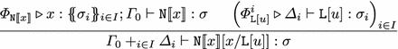
Lemma 10

(Partial Substitution). If ${\varPhi _{\mathtt{N}{[} \! {[} x {]} \! {]}}} \triangleright _{\mathcal{A}} {{x{:} \{ \! \! \{ \sigma _i \} \! \! \} _{i \in I};\varGamma } \vdash \mathtt{N}{[} \! {[} x {]} \! {]}{:}\tau }$ and $({\varPhi _u^i} \triangleright _{\mathcal{A}} {{\varDelta _i} \vdash u{:}\sigma _i})_{ i \in I}$ then $\exists \varPhi _{\mathtt{N}{[} \! {[} u {]} \! {]}}$ s.t. ${\varPhi _{\mathtt{N}{[} \! {[} u {]} \! {]}}} \triangleright _{\mathcal{A}} {{x{:} \{ \! \! \{ \sigma _i \} \! \! \} _{ i \in I\backslash K}; \varGamma +_{k \in K} \varDelta _k} \vdash \mathtt{N}{[} \! {[} u {]} \! {]}{:}\tau }$, for some $K \subseteq I$ where $\mathtt {sz}(\varPhi _{\mathtt{N}{[} \! {[} u {]} \! {]}}) = \mathtt {sz}(\varPhi _{\mathtt{N}{[} \! {[} x {]} \! {]}}) +_{k \in K} \mathtt {sz}(\varPhi _u^k) - |K|$.

Proof

By induction on typing derivations (a similar proof appears in [17]). $\Diamond$

To complete the subject reduction argument we still need to guarantee that every needed variable of a typed term is necessarily typed, a property which is specified by means of the following lemma.

Lemma 11

If $\varPhi \triangleright _{\mathcal{A}} {\varGamma } \vdash \mathtt{N}{[} \! {[} x {]} \! {]}{:}\tau$, then $\exists \varGamma '$, $\exists I \ne \emptyset$, and $\exists (\sigma _i)_{i \in I}$ such that $\varGamma = x: \{ \! \! \{ \sigma _i \} \! \! \} _{i \in I}; \varGamma '$.

Proof

By induction on $\mathtt{N}$. The base case $\mathtt{N}=\Box$ is straightforward. We only show here the interesting inductive case $\mathtt{N}{[} \! {[} x {]} \! {]} = \mathtt{N}_1 {[} \! {[} y {]} \! {]}[y/\mathtt{N}_2{[} \! {[} x {]} \! {]}]$, for which $\varPhi$ has necessarily the following form, where $\varGamma = \varPi +_{j \in J} \varDelta _j$.

By the i.h. on the left derivation we have $J \ne \emptyset$. By the i.h. on the right derivations $\varDelta _j = x: \{ \! \! \{ \tau ^i_j \} \! \! \} _{i \in I_j}; \varDelta '_j$ and $I_j \ne \emptyset$ for all $j \in J$. Moreover, $\varPi = x: \{ \! \! \{ \tau _k \} \! \! \} _{k \in K}; \varPi '$, where K could be empty. Then

The property then holds for $\{ \! \! \{ \sigma _i \} \! \! \} _{i \in I} = \{ \! \! \{ \tau _k \} \! \! \} _{k \in K} +_{j \in J} \{ \! \! \{ \tau ^i_j \} \! \! \} _{i \in I_j}$ and $\varGamma ' = \varPi ' +_{j \in J} \varDelta '_j$. We have $I \ne \emptyset$ since $J \ne \emptyset$ and $I_j \ne \emptyset$ for all $j \in J$. $\Diamond$

Subject reduction can now be stated in a combinatorial way, by using the $\mathtt {sz}(\_)$ measure on derivations defined in Sect. 3.

Theorem 4

(Weighted Subject Reduction for $\mathtt{need}$ ). Let ${\varPhi } \triangleright _{\mathcal{A}} {{\varGamma } \vdash t{:}\tau }$. If $t \rightarrow _{\mathtt{need}} t'$, then there exists $\varPhi '$ s.t. ${\varPhi '} \triangleright _{\mathcal{A}} {{\varGamma } \vdash t'{:}\tau }$. Moreover, $\mathtt {sz}(\varPhi ) > \mathtt {sz}(\varPhi ')$.

Proof

By induction on $t \rightarrow _{\mathtt{need}} t'$, using Lemmas 8, 9, 10 and 11. We refer the interested reader to the Appendix for full details of the proof. $\Diamond$

To show that $\mathtt{need}$-normalizing terms are $\mathcal{A}$-typable we use a subject expansion property, which needs the following lemma.

Lemma 12

(Reverse Partial Substitution). Let $\mathtt{N}{[} \! {[} x {]} \! {]}, s$ be terms s.t. $x \notin \mathtt{fv}(s)$ and ${\varPhi _{\mathtt{N}{[} \! {[} s {]} \! {]}}} \triangleright _{\mathcal{A}} {{\varGamma } \vdash \mathtt{N}{[} \! {[} s {]} \! {]}{:}\tau }$. Then $\exists \varGamma _0$, $\exists \varPhi _{\mathtt{N}{[} \! {[} x {]} \! {]}}$, $\exists I$, $\exists (\varDelta _i)_{i \in I}$, $\exists (\sigma _i)_{i \in I}$, $\exists (\varPhi ^i_s)_{i \in I}$ s.t. $\varGamma = \varGamma _0 +_{i \in I} \varDelta _i$ and ${\varPhi _{\mathtt{N}{[} \! {[} x {]} \! {]}}} \triangleright _{\mathcal{A}} {{x: \{ \! \! \{ \sigma _i \} \! \! \} _{i \in I} + \varGamma _0} \vdash \mathtt{N}{[} \! {[} x {]} \! {]}{:}\tau }$ and $({\varPhi ^i_s} \triangleright _{\mathcal{A}} {{\varDelta _i} \vdash s{:}\sigma _i})_{i \in I}$.

Proof

By induction on the structure of $\mathtt{N}{[} \! {[} s {]} \! {]}$.

• If $\mathtt{N}= \Box$, then $\mathtt{N}{[} \! {[} s {]} \! {]} = s$ and the result holds, for $\varGamma _0 = \emptyset$, $|I| = 1$ and $\sigma _1 = \tau$.

• If $\mathtt{N}= \lambda y. \mathtt{M}$ then the property is straightforward by the i.h. (since $y \notin \mathtt{fv}(s)$ by $\alpha$-conversion).

• If $\mathtt{N}= \mathtt{M}r$ then $\mathtt{N}{[} \! {[} s {]} \! {]} = \mathtt{M}{[} \! {[} s {]} \! {]} r$ and by construction $\varGamma = \varPi +_{j \in J} \varGamma _j$ and ${\varPhi _{\mathtt{M}{[} \! {[} s {]} \! {]}}} \triangleright {{\varPi } \vdash \mathtt{M}{[} \! {[} s {]} \! {]}{:}{ \{ \! \! \{ \rho _j \} \! \! \} _{j \in J}}\!\rightarrow \!{\tau }}$ and $({\varPhi ^j_r} \triangleright {{\varGamma _j} \vdash r{:}\rho _j})_{j \in J}$. By the i.h. $\varPi = \varPi _0 +_{i \in I} \varDelta _i$ where ${x: \{ \! \! \{ \sigma _i \} \! \! \} _{i \in I} + \varPi _0} \vdash \mathtt{M}{[} \! {[} x {]} \! {]}{:}{ \{ \! \! \{ \rho _j \} \! \! \} _{j \in J}}\!\rightarrow \!{\tau }$ and $({\varDelta _i} \vdash s{:}\sigma _i)_{i \in I}$. Then, by the rule $(\rightarrow {\text{ e }})$, ${x: \{ \! \! \{ \sigma _i \} \! \! \} _{i \in I} + \varPi _0 +_{j \in J} \varGamma _j} \vdash \mathtt{M}{[} \! {[} x {]} \! {]} r{:}\tau$. The result then holds for $\varGamma _0 := \varPi _0 +_{j \in J} \varGamma _j$.

• If $\mathtt{N}= r \mathtt{M}$ then $\mathtt{N}{[} \! {[} s {]} \! {]} = r \mathtt{M}{[} \! {[} s {]} \! {]}$ and by construction $\varGamma = \varPi +_{j \in J} \varGamma _j$ and ${\varPhi _r} \triangleright {{\varPi } \vdash r{:}{ \{ \! \! \{ \rho _j \} \! \! \} _{j \in J}}\!\rightarrow \!{\tau }}$ and $({\varPhi ^j_{\mathtt{M}{[} \! {[} s {]} \! {]}}} \triangleright {{\varGamma _j} \vdash \mathtt{M}{[} \! {[} s {]} \! {]}{:}\rho _j})_{j \in J}$. By the i.h. for each $j \in J$, $\varGamma _j = \varGamma ^j_0 +_{i \in I_j} \varGamma ^j_i$ where ${x: \{ \! \! \{ \sigma _i \} \! \! \} _{i \in I_j} + \varGamma ^j_0} \vdash \mathtt{M}{[} \! {[} x {]} \! {]}{:}\rho _j$ and $({\varGamma ^j_i} \vdash s{:}\sigma _i)_{i \in I_j}$. Let $I := \cup _{j \in J} I_j$. Then, by the rule $(\rightarrow {\text{ e }})$, ${\varPi +_{j \in J} (x: \{ \! \! \{ \sigma _i \} \! \! \} _{i \in I_j} + \varGamma ^j_0)} \vdash r \mathtt{M}{[} \! {[} x {]} \! {]}{:}\tau$. Note that $\varPi +_{j \in J} (x: \{ \! \! \{ \sigma _i \} \! \! \} _{i \in I_j} + \varGamma ^j_0) = x: \{ \! \! \{ \sigma _i \} \! \! \} _{i \in I} + \varPi +_{j \in J} \varGamma ^j_0$. The result then holds for $\varGamma _0 := \varPi +_{j \in J} \varGamma ^j_0$.

• All the remaining cases are similar to the previous ones. $\Diamond$

Theorem 5

(Subject Expansion for $\mathtt{need}$ ). Let ${\varPhi '} \triangleright _{\mathcal{A}} {{\varGamma } \vdash t'{:}\tau }$. If $t \rightarrow _{\mathtt{need}} t'$, then there exists $\varPhi$ s.t. ${\varPhi } \triangleright _{\mathcal{A}} {{\varGamma } \vdash t{:}\tau }$.

Proof

By induction on $\varPhi '$ using Lemmas 8, 9 and 12. $\Diamond$

To state the full characterization result of this section, we still need to relate typing of $\mathcal{T}_{\mathtt{e}}$-terms in system $\mathcal{A}$ with typing of $\mathcal{T}_{\mathtt{a}}$-terms in system $\mathcal{V}$.

Lemma 13

Let $t \in \mathcal{T}_{\mathtt{e}}$. Then ${\varPhi } \triangleright _{\mathcal{V}} {{\varGamma } \vdash { t}^{\downarrow }{:}\sigma }$ implies ${\varPhi '} \triangleright _{\mathcal{A}} {{\varGamma } \vdash t{:}\sigma }$.

Proof

By induction on t.

• If $t=x$, then ${ t}^{\downarrow } = x$. The derivation $\varPhi$ has the form ${x: \{ \! \! \{ \sigma \} \! \! \} } \vdash x{:}\sigma$ so that $\varPhi '$ has also the form ${x: \{ \! \! \{ \sigma \} \! \! \} } \vdash x{:}\sigma$.

• If $t=\lambda x. u$, then ${ t}^{\downarrow } = \lambda x. { u}^{\downarrow }$. We have $\varGamma = \varDelta \setminus \!\!\!\setminus \, x$ and $\sigma = {\varDelta (x)}\!\rightarrow \!{\tau }$, where ${\varDelta \setminus \!\!\!\setminus \, x} \vdash \lambda x. { u}^{\downarrow }{:}{\varDelta (x)}\!\rightarrow \!{\tau }$ is necessarily derivable from a derivation ${\varPhi _u} \triangleright _{\mathcal{V}} {{\varDelta } \vdash { u}^{\downarrow }{:}\tau }$. The i.h. gives ${\varPhi '_u} \triangleright _{\mathcal{A}} {{\varDelta } \vdash u{:}\tau }$ so that we construct ${\varPhi '} \triangleright _{\mathcal{A}} {{\varDelta \setminus \!\!\!\setminus \, x} \vdash \lambda x. u{:}{\varDelta (x)}\!\rightarrow \!{\tau }}$ which concludes the proof.

• If $t=t_1 t_2$, then the proof proceeds by induction as in the previous case.

• If $t=t_1[x/ t_2]$, then ${ t}^{\downarrow } = { t_1}^{\downarrow }\{ x/ { t_2}^{\downarrow } \}$. By Lemma 7 we know that $\varGamma = \varGamma _0 +_{i \in I} \varDelta _i$ and ${\varPhi _{{ t_1}^{\downarrow }}} \triangleright _{\mathcal{V}} {{x: \{ \! \! \{ \sigma _i \} \! \! \} _{i \in I};\varGamma _0} \vdash { t_1}^{\downarrow }{:}\tau }$ and $({\varPhi ^i_{{ t_2}^{\downarrow }}} \triangleright _{\mathcal{V}} {{\varDelta _i} \vdash { t_2}^{\downarrow }{:}\sigma _i})_{i \in I}$. The i.h. then gives ${\varPhi '_{t_1}} \triangleright _{\mathcal{A}} {{x: \{ \! \! \{ \sigma _i \} \! \! \} _{i \in I};\varGamma _0} \vdash t_1{:}\tau }$ and $({\varPhi '^i_{t_2}} \triangleright _{\mathcal{A}} {{\varDelta _i} \vdash t_2{:}\sigma _i})_{i \in I}$. We then conclude ${\varPhi '_{t}} \triangleright _{\mathcal{A}} {{\varGamma } \vdash t_1[x/t_2]{:}\tau }$ by using rule $(\mathtt{cut})$. $\Diamond$

We can now state the full characterization result, which is one of the main results of this paper. The implication “typable terms in system $\mathcal{A}$ are $\mathtt{need}$-normalizing” is obtained through the weighted subject reduction, which provides a completely combinatorial argument of this property, as in the call-by-name case. This is exactly the advantage provided by the quantitative approach based on non-idempotent types, which makes the difference with a qualitative system based on idempotent intersection types.

Theorem 6

Let $t \in \mathcal{T}_{\mathtt{e}}$. Then, ${\varPhi } \triangleright _{\mathcal{A}} {{\varGamma } \vdash t{:}\tau }$ iff $t\in \mathcal{WN}(\mathtt{need})$.

Proof

Let $\varPhi \triangleright {\varGamma } \vdash t{:}\tau$. Then $\mathtt{need}$-reduction necessarily terminates by Theorem 4 so that $t\in \mathcal{WN}(\mathtt{need})$.

Let $t \in \mathcal{WN}(\mathtt{need})$, so that $t \twoheadrightarrow _{\mathtt{need}}^k t'$, where $t' \in \mathtt{need}$-nf. We proceed by induction on k. If $k=0$ (i.e. $t=t'$), then t is in $\mathtt{need}$-nf. By Lemma 3 ${ t}^{\downarrow }$ is in $\mathtt{name}$-nf. Then ${\varPhi } \triangleright _{\mathcal{V}} {{\varGamma } \vdash { t}^{\downarrow }{:}\sigma }$ by Theorem 3 and ${\varPhi } \triangleright _{\mathcal{A}} {{\varGamma } \vdash t{:}\sigma }$ by Lemma 13.

Otherwise, let $t \rightarrow _{\mathtt{need}} u \rightarrow _{\mathtt{need}}^k t'$. By the i.h. we have ${\varPhi '} \triangleright _{\mathcal{A}} {{\varGamma } \vdash u{:}\tau }$, thus by Theorem 5 we obtain ${\varPhi } \triangleright _{\mathcal{A}} {{\varGamma } \vdash t{:}\tau }$. $\Diamond$

6 Soundness and Completeness

This section uses the two characterization results developed in Sects. 4 and 5 to prove soundness and completeness of call-by-need w.r.t call-by-name. More precisely, a call-by-name interpreter stops in a value if and only if the call-by-need interpreter stops in an answer. This implies that call-by-need and call-by-name are observationally equivalent, so that in particular call-by-need turns out to be a correct implementation of call-by-name.

Lemma 14

Let $t \in \mathcal{T}_{\mathtt{a}}$. Then $t \in \mathcal{WN}(\mathtt{need}) \Leftrightarrow t \in \mathcal{WN}(\mathtt{name})$.

Proof

Let $t \in \mathcal{WN}(\mathtt{need})$. Then $\varPhi \triangleright _{\mathcal{A}} {\varGamma } \vdash t{:}\tau$ holds by Theorem 6, and $\varPhi \triangleright _{\mathcal{V}} {\varGamma } \vdash t{:}\tau$ holds by Lemma 4, thus we get $t \in \mathcal{WN}(\mathtt{name})$ by Theorem 3. Conversely, let $t \in \mathcal{WN}(\mathtt{name})$. Then $\varPhi \triangleright _{\mathcal{V}} {\varGamma } \vdash t{:}\tau$ holds by Theorem 3, so that $\varPhi \triangleright _{\mathcal{A}} {\varGamma } \vdash t{:}\tau$ holds by Lemma 4, and thus we get $t \in \mathcal{WN}(\mathtt{need})$ by Theorem 6. $\Diamond$

Given a reduction relation $\mathcal {R}$ on a term language $\mathcal{T}$, and an associated notion of context for the term language $\mathcal{T}$, we define t to be observationally equivalent to u, written $t \cong _{\mathcal {R}} u$, if and only if $\mathtt{C}[t] \in \mathcal{WN}(\mathcal {R}) \Leftrightarrow \mathtt{C}[s] \in \mathcal{WN}(\mathcal {R})$ for every context $\mathtt{C}$. Since we work with two different term languages $\mathcal{T}_{\mathtt{a}}$ and $\mathcal{T}_{\mathtt{e}}$, we first need to introduce their associated notions of contexts $\mathtt{C}$ and $\mathtt{C}'$, which represent, respectively, contexts without and with explicit substitutions.

We can thus conclude with the last main result of the paper.

Corollary 1

For all terms t and u in $\mathcal{T}_{\mathtt{a}}$, $t \cong _{\mathtt{name}} u$ iff $t \cong _{\mathtt{need}} u$.

Proof

First of all let us consider the relation $=_{\mathtt{B}}$, which is the least equivalence relation generated by the axiom $(\lambda x. t_1) t_2 = t_1[x/t_2]$. We remark that when t is typable in $\mathcal{A}$, and $t =_{\mathtt{B}} t'$, then $t'$ is typable in $\mathcal{A}$. This means that we can indistinctly quantify over the two sort of contexts $\mathtt{C}$ and $\mathtt{C}'$ previously defined: indeed, from the set of all the contexts $\mathtt{C}$ we can construct the set of all the contexts $\mathtt{C}'$, and vice-versa. The proof of the corollary then proceeds as follows. Take $t, u \in \mathcal{T}_{\mathtt{a}}$. Then $t \cong _{\mathtt{name}} u$ iff (definition)

$\mathtt{C}[t] \in \mathcal{WN}(\mathtt{name}) \Leftrightarrow \mathtt{C}[u] \in \mathcal{WN}(\mathtt{name})$ for every context $\mathtt{C}$ iff (Theorem 3)

$\mathtt{C}[t]$ is typable in $\mathcal{V}\Leftrightarrow \mathtt{C}[u]$ is typable in $\mathcal{V}$ for every context $\mathtt{C}$ iff (Lemma 4)

$\mathtt{C}[t]$ is typable in $\mathcal{A}\Leftrightarrow \mathtt{C}[u]$ is typable in $\mathcal{A}$ for every context $\mathtt{C}$ iff (Remark)

$\mathtt{C}'[t]$ is typable in $\mathcal{A}\Leftrightarrow \mathtt{C}'[u]$ is typable in $\mathcal{A}$ for every context $\mathtt{C}'$ iff (Theorem 6)

$\mathtt{C}'[t] \in \mathcal{WN}(\mathtt{need}) \Leftrightarrow \mathtt{C}'[u] \in \mathcal{WN}(\mathtt{need})$ for every context $\mathtt{C}'$ iff (definition) $t \cong _{\mathtt{need}} u$. $\Diamond$

7 Conclusion

This paper gives the first full characterization of call-by-need normalization by means of intersection types. This result, together with the full characterization of call-by-name normalization, provides a new completeness proof for call-by-need, which is only based on logical arguments and does not make use of any complicated notion of rewriting. The use of non-idempotent types allows us to obtain the result in a combinatorial way, by providing quantitative information about reduction sequences, and without resorting to any reducibility argument.

The paper only considers a core language for call-by-need, but it would be interesting to consider other constructors of lazy languages, e.g. data constructors, case-expressions and Haskell’s seq operators. Moreover, the results in the paper could be extended to the cyclic call-by-need letrec calculus as well as to full (strong) need normal forms (ongoing work).

Last but not least, we would also like to use the ideas in [16] in order to relate call-by-need and needed reduction by means of intersection types.

A Appendix

Lemma 9

If $({\varPhi ^j_{\mathtt{L}}} \triangleright _{\mathcal{A}} { \varGamma _j \Vdash \mathtt{L}\triangleright \varDelta _j})_{j \in J}$, then ${\varPhi _{\mathtt{L}}} \triangleright _{\mathcal{A}} {+_{j \in J} \varGamma _j \Vdash \mathtt{L}\triangleright +_{j \in J} \varDelta _j}$. Moreover, $\mathtt {sz}(\varPhi _{\mathtt{L}}) = +_{j \in J} \mathtt {sz}(\varPhi ^j_{\mathtt{L}}) - (\mathtt{height}(\mathtt{L}) \cdot (|J| - 1))$.

Proof

The proof is by induction on $\mathtt{L}$. The case $\mathtt{L}= \Box$ is straightforward since $\varGamma _j = \varDelta _j = \emptyset$ so that $+_{j \in J} \varGamma _j = +_{j \in J} \varDelta _j = \emptyset$. We have $\mathtt {sz}(\varPhi _{\Box }) = 1 = |J| - |J| +1 = |J| - [1 \cdot (|J| - 1) ] = +_{j \in J} \mathtt {sz}(\varPhi ^j_{\Box }) - (\mathtt{height}(\Box ) \cdot (|J| - 1))$.

Let $\mathtt{L}= \mathtt{L}' [y/u]$. Then for each $j \in J$, the derivation $\varPhi ^j_{\mathtt{L}}$ has the following form, where $\varGamma _j = \varPi _j +_{i \in K_j \uplus H_j} \Lambda ^j_k$ and $\varDelta _j = \varDelta '_j; y: \{ \! \! \{ \sigma _h \} \! \! \} _{h \in H_j}$.

By the i.h. we have ${\varPhi _{\mathtt{L}'}} \triangleright {+_{j \in J} (y: \{ \! \! \{ \sigma _k \} \! \! \} _{k \in K_j} ; \varPi _j) \Vdash \mathtt{L}' \triangleright +_{j \in J} \varDelta '_j}$, but $+_{j \in J} (y: \{ \! \! \{ \sigma _k \} \! \! \} _{k \in K_j} ; \varPi _j) = y: \{ \! \! \{ \sigma _k \} \! \! \} _{j \in J, k \in K_j} ; +_{j \in J} \varPi _j$. We thus construct the derivation $\varPhi _{\mathtt{L}}$:

We conclude with the first statement since $+_{j \in J} \varGamma _j = +_{j \in J} \varPi _j +_{j \in J, i \in K_j \uplus H_j} \varLambda ^j_k$ and $+_{j \in J} \varDelta _j = +_{j \in J} \varDelta '_j,y: \{ \! \! \{ \sigma _h \} \! \! \} _{j \in J, h \in H_j}$. Moreover:

$\begin{array}{ll} \mathtt {sz}(\varPhi _{\mathtt{L}}) = \mathtt {sz}(\varPhi _{\mathtt{L}'}) +_{j \in J, i \in K_j \uplus H_j} \mathtt {sz}(\varPhi _{\Psi ^{j,i}_u}) +1 &{} =_{{ i.h.}} \\ +_{j \in J} \mathtt {sz}(\varPhi _{\mathtt{L}'}) - (\mathtt{height}(\mathtt{L}') \cdot (|J| -1 ) ) +_{j \in J, i \in K_j \uplus H_j} \mathtt {sz}(\varPhi _{\Psi ^{j,i}_u}) +1 &{} =_{{ i.h.}} \\ +_{j \in J} \mathtt {sz}(\varPhi _{\mathtt{L}'})+_{j \in J, i \in K_j \uplus H_j} \mathtt {sz}(\varPhi _{\Psi ^{j,i}_u}) + |J| - [(\mathtt{height}(\mathtt{L}') +1)\cdot (|J| -1 )] &{} = \\ +_{j \in J} \mathtt {sz}(\varPhi _{\mathtt{L}}) - (\mathtt{height}(\mathtt{L}) \cdot (|J| -1 )) &{} \Diamond \\ \end{array}$

Theorem 4

(Weighted Subject Reduction for $\mathtt{need}$ ). Let ${\varPhi } \triangleright _{\mathcal{A}} {{\varGamma } \vdash t{:}\tau }$. If $t \rightarrow _{\mathtt{need}} t'$, then there exists $\varPhi '$ s.t. ${\varPhi '} \triangleright _{\mathcal{A}} {{\varGamma } \vdash t'{:}\tau }$. Moreover, $\mathtt {sz}(\varPhi ) > \mathtt {sz}(\varPhi ')$.

Proof

By induction on $t \rightarrow _{\mathtt{need}} t'$.

• If $t = \mathtt{L}[\lambda x. u] s \rightarrow _{\mathtt{dB}} \mathtt{L}[u[x/s]] = t'$, then one shows ${\varPhi '} \triangleright {{\varGamma } \vdash t'{:}\tau }$ and $\mathtt {sz}(\varPhi ) > \mathtt {sz}(\varPhi ')$ by induction on $\mathtt{L}$. See the first case of Lemma 2 in [17] (pp. 19).

• If $t = \mathtt{N}{[} \! {[} x {]} \! {]}[x/ \mathtt{L}[u]] \rightarrow _{\mathtt{lsv}} \mathtt{L}[\mathtt{N}{[} \! {[} u {]} \! {]}[x/u]] = t'$, then the derivation $\varPhi$ has the following form, where $\varGamma = \varGamma _0 +_{i \in I} \varDelta _i$.

  

  By Lemma 8, for all $i \in I$, there exist $\varPi ^i_1, \varPi ^i_2, \varPi ^i_3$ such that ${\varPhi ^i_{\mathtt{L}}} \triangleright {\varPi ^i_1 \Vdash \mathtt{L}\triangleright \varPi ^i_2}$, ${\varPhi ^i_u} \triangleright {\varPi ^i_2; \varPi ^i_3 \vdash u: \sigma _i}$ and $\varDelta _i = \varPi ^i_1 + \varPi ^i_3$.

  Then, from the derivations $\varPhi _{\mathtt{N}{[} \! {[} x {]} \! {]}}$ and $(\varPhi ^i_u)_{i \in I}$ we get, by Lemma 10, a derivation ${\varPhi _{\mathtt{N}{[} \! {[} u {]} \! {]}}} \triangleright {x: \{ \! \! \{ \sigma _i \} \! \! \} _{i \in I\setminus K}; \varGamma _0 +_{k \in K} (\varPi ^k_2; \varPi ^k_3) \vdash \mathtt{N}{[} \! {[} u {]} \! {]} : \sigma }$ for some $K \subseteq I$. Therefore, we can construct the following derivation $\varPhi _{\mathtt{N}{[} \! {[} u {]} \! {]}[x/u]}$.

  

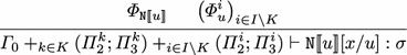
  The last sequent can be written $\varGamma _0 + ( +_{i \in I} \varPi ^i_2; +_{i \in I} \varPi ^i_3) \vdash \mathtt{N}{[} \! {[} u {]} \! {]}[x/u]:\sigma$.

  Now, from $\varPhi _{\mathtt{N}{[} \! {[} x {]} \! {]}}$ and Lemma 11 we know that $I \ne \emptyset$. We can thus apply Lemma 9 to $(\varPhi ^i_{\mathtt{L}})_{i \in I}$ and we get ${\varPhi _{\mathtt{L}}} \triangleright {+_{i \in I}\varPi ^i_1 \Vdash \mathtt{L}\triangleright +_{i \in I} \varPi ^i_2}$. We can thus apply Lemma 8 to $\varPhi _{\mathtt{L}}$ and $\varPhi _{\mathtt{N}{[} \! {[} u {]} \! {]}[x/u]}$, obtaining ${\varPhi '} \triangleright {\varGamma _0 +_{i \in I} \varPi ^1_1 +_{i \in I} \varPi ^i_3 \vdash L[\mathtt{N}{[} \! {[} u {]} \! {]}[x/u]]:\sigma }$.

  We can then conclude with the first statement since $\varGamma _0 +_{i \in I} \varPi ^1_1 +_{i \in I} \varPi ^i_3 = \varGamma _0 +_{i \in I} \varDelta _i = \varGamma$ as required. Moreover, for the second one, we have two equalities:

  $$ \begin{array}{ll} \mathtt {sz}(\varPhi ) = \mathtt {sz}(\varPhi _{\mathtt{N}{[} \! {[} x {]} \! {]} }) +_{i \in I} \mathtt {sz}(\varPhi ^i_{\mathtt{L}[u]}) +1 &{} =_{L. 8} \\ \mathtt {sz}(\varPhi _{\mathtt{N}{[} \! {[} x {]} \! {]} }) +_{i \in I} (\mathtt {sz}(\varPhi ^i_{\mathtt{L}}) + \mathtt {sz}(\varPhi ^i_u) -1) +1 &{} = \\ \mathtt {sz}(\varPhi _{\mathtt{N}{[} \! {[} x {]} \! {]} }) +_{i \in I} \mathtt {sz}(\varPhi ^i_{\mathtt{L}}) +_{i \in I} \mathtt {sz}(\varPhi ^i_u) - (|I| -1 ) &{} = Z - (|I| -1 ) \\ \end{array} $$

  and

  $$ \begin{array}{ll} \mathtt {sz}(\varPhi ') =_{L. 8} \mathtt {sz}(\varPhi _{\mathtt{L}}) + \mathtt {sz}(\varPhi _{\mathtt{N}{[} \! {[} u {]} \! {]}[x/u]}) -1 &{} = \\ \mathtt {sz}(\varPhi _{\mathtt{L}}) + \mathtt {sz}(\varPhi _{\mathtt{N}{[} \! {[} u {]} \! {]}}) +_{i \in I\setminus K} \mathtt {sz}(\varPhi ^i_{u}) +1 -1 &{} = \\ \mathtt {sz}(\varPhi _{\mathtt{L}}) + \mathtt {sz}(\varPhi _{\mathtt{N}{[} \! {[} u {]} \! {]}}) +_{i \in I\setminus K} \mathtt {sz}(\varPhi ^i_{u}) &{} =_{L. 10} \\ \mathtt {sz}(\varPhi _{\mathtt{L}}) + \mathtt {sz}(\varPhi _{\mathtt{N}{[} \! {[} x {]} \! {]}}) +_{k \in K} \mathtt {sz}(\varPhi ^k_{u}) - |K| +_{i \in I\setminus K} \mathtt {sz}(\varPhi ^i_{u}) &{} =_{L. 9} \\ +_{i \in I} \mathtt {sz}(\varPhi ^i_{\mathtt{L}}) - [\mathtt{height}(\mathtt{L}) \cdot (|I| - 1)] + \mathtt {sz}(\varPhi _{\mathtt{N}{[} \! {[} x {]} \! {]}}) +_{i \in I} \mathtt {sz}(\varPhi ^i_{u}) - |K| &{} = \\ \mathtt {sz}(\varPhi _{\mathtt{N}{[} \! {[} x {]} \! {]} }) +_{i \in I} \mathtt {sz}(\varPhi ^i_{\mathtt{L}}) +_{i \in I} \mathtt {sz}(\varPhi ^i_u) - [\mathtt{height}(\mathtt{L}) \cdot (|I| - 1)] - |K| &{} = \\ Z- [\mathtt{height}(\mathtt{L}) \cdot (|I| - 1)] - |K| &{} \\ \end{array} $$

  To conclude, we know by Lemma 10 that $K \ne \emptyset$. Therefore, $|I| -1 \le \mathtt{height}(\mathtt{L}) \cdot (|I| - 1)$ so that $Z - (|I| -1 ) \ge Z - [\mathtt{height}(\mathtt{L}) \cdot (|I| - 1)] > Z - [\mathtt{height}(\mathtt{L}) \cdot (|I| - 1)] - |K|$. We thus conclude $\mathtt {sz}(\varPhi )> \mathtt {sz}(\varPhi ')$ as required.

• If $t = \mathtt{N}_1 {[} \! {[} x {]} \! {]}[x/ \mathtt{N}_2[u]] \rightarrow _{\mathtt{need}} \mathtt{N}_1 {[} \! {[} x {]} \! {]}[x/ \mathtt{N}_2[u']] =t'$ comes from $\mathtt{N}[u] \rightarrow _{\mathtt{need}} \mathtt{N}[u']$, then $\varPhi$ has the following form, where $\varGamma = \varGamma _0 +_{i \in I} \varDelta _i$.

  

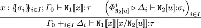
  By the i.h. both ${\varPi ^i_{\mathtt{N}_2[u]}} \triangleright {{\varDelta _i} \vdash \mathtt{N}_2[u']{:}\sigma _i}$ and $\mathtt {sz}(\varPhi ^i_{\mathtt{N}_2[u]}) > \mathtt {sz}(\varPi ^i_{\mathtt{N}_2[u]})$ hold for all $i \in I$. The first statement gives ${\varPhi '} \triangleright {{\varGamma _0 +_{i \in I} \varDelta _i} \vdash \mathtt{N}_1 {[} \! {[} x {]} \! {]}[x/ \mathtt{N}_2[u']]{:}\tau }$. The second one gives $\mathtt {sz}(\varPhi ) > \mathtt {sz}(\varPhi ')$ since $I \ne \emptyset$ holds by Lemma 11.

• The cases $t = \mathtt{N}[u]v \rightarrow _{\mathtt{need}} \mathtt{N}[u']v =t'$ and $t = \mathtt{N}[u][x/v] \rightarrow _{\mathtt{need}} \mathtt{N}[u'][x/v] =t'$ coming from $\mathtt{N}[u] \rightarrow _{\mathtt{need}} \mathtt{N}[u']$ are straightforward inductive cases. $\Diamond$

References

Accattoli, B., Barenbaum, P., Mazza, D.: Distilling abstract machines. In: ICFP. ACM Press (2014)
Ariola, Z.M., Felleisen, M.: The call-by-need lambda calculus. J. Funct. Program. 7(3), 265–301 (1997)
Ariola, Z.M., Felleisen, M., Maraist, J., Odersky, M., Wadler, P.: The call-by-need lambda calculus. In: POPL, pp. 233–246. ACM Press (1995)
Barendregt, H., Coppo, M., Dezani-Ciancaglini, M.: A filter lambda model and the completeness of type assignment. Bull. Symbolic Logic 48, 931–940 (1983)
Bernadet, A., Lengrand, S.: Non-idempotent intersection types and strong normalisation. Logical Methods Comput. Sci. 9(4:3), 1–46 (2013)
Boudol, G., Curien, P.-L., Lavatelli, C.: A semantics for lambda calculi with resources. Math. Struct. Comput. Sci. 9(4), 437–482 (1999)
Bucciarelli, A., Kesner, D., Ronchi Della Rocca, S.: The inhabitation problem for non-idempotent intersection types. In: Diaz, J., Lanese, I., Sangiorgi, D. (eds.) TCS 2014. LNCS, vol. 8705, pp. 341–354. Springer, Heidelberg (2014)
Cardone, F., Coppo, M.: Two extension of Curry’s type inference system. In: Odifreddi, P. (ed.) Logic and Computer Science. APIC Series, vol. 31, pp. 19–75. Academic Press, New York (1990)
Chang, S., Felleisen, M.: The call-by-need lambda calculus, revisited. In: Seidl, H. (ed.) ESOP 2012. LNCS, vol. 7211, pp. 128–147. Springer, Heidelberg (2012)
Coppo, M., Dezani-Ciancaglini, M., Venneri, B.: Functional characters of solvable terms. Math. Logic Q. 27(2–6), 45–58 (1981)
Coppo, M., Dezani-Ciancaglini, M.: A new type-assignment for lambda terms. Archiv für Math. Logik Grundlagenforschung 19, 139–156 (1978)
Coppo, M., Dezani-Ciancaglini, M.: An extension of the basic functionality theory for the \(\lambda \)-calculus. Notre Dame J. Formal Logic 21, 685–693 (1980)
Danvy, O., Zerny, I.: A synthetic operational account of call-by-need evaluation. In: PPDP, pp. 97–108. ACM Press (2013)
De Benedetti, E., Ronchi Della Rocca, S.: Bounding normalization time through intersection types. In: ITRS 2012, EPTCS, pp. 48–57 (2013)
de Carvalho, D.: Sémantiques de la logique linéaire et temps de calcul. Thèse de doctorat, Université Aix-Marseille II (2007)
Gardner, P.: Discovering needed reductions using type theory. In: Hagiya, M., Mitchell, J.C. (eds.) TACS 1994. LNCS, vol. 789, pp. 555–574. Springer, Heidelberg (1994)
Kesner, D., Ventura, D.: Quantitative types for intuitionistic calculi. Technical report (2014). https://hal.archives-ouvertes.fr/hal-00980868
Kesner, D., Ventura, D.: Quantitative types for the linear substitution calculus. In: Diaz, J., Lanese, I., Sangiorgi, D. (eds.) TCS 2014. LNCS, vol. 8705, pp. 296–310. Springer, Heidelberg (2014)
Kfoury, A.J.: A linearization of the lambda-calculus and consequences. Technical report, Boston Universsity (1996)
Kfoury, A.J.: A linearization of the lambda-calculus and consequences. J. Logic Comput. 10(3), 411–436 (2000)
Kfoury, A.J., Wells, J.B.: Principality and type inference for intersection types using expansion variables. Theor. Comput. Sci. 311(1–3), 1–70 (2004)
Krivine, J.-L.: Lambda-Calculus, Types and Models. Ellis Horwood, Hemel Hempstead (1993)
Mairson, H., Neergaard, P.M.: Types, potency, idempotency: why nonlinearity and amnesia make a type system work. In: ICFP, pp. 138–149. ACM (2004)
Maraist, J., Odersky, M., Turner, D.N., Wadler, P.: Call-by-name, call-by-value, call-by-need and the linear lambda calculus. Theoret. Comput. Sci. 228(1–2), 175–210 (1999)
Maraist, J., Odersky, M., Wadler, P.: The call-by-need lambda calculus. J. Funct. Program. 8(3), 275–317 (1998)
Pagani, M., Ronchi Della Rocca, S.: Linearity, non-determinism and solvability. Fundam. Informaticae 103, 358–373 (2010)
Pagani, M., della Rocca, S.R.: Solvability in resource lambda-calculus. In: Ong, L. (ed.) FOSSACS 2010. LNCS, vol. 6014, pp. 358–373. Springer, Heidelberg (2010)
Plotkin, G.D.: Call-by-Name, call-by-value and the lambda-calculus. Theor. Comput. Sci. 1(2), 125–159 (1975)
van Bakel, S.: Complete restrictions of the intersection type discipline. Theor. Comput. Sci. 102(1), 135–163 (1992)
Wadsworth, C.: Semantics and Pragmatics of the Lambda Calculus. PH.D. thesis, Oxford University (1971)
Author information
Authors and Affiliations
Corresponding author
Editor information
Editors and Affiliations