Nearly Optimal Verifiable Data Streaming

Abstract

The problem of verifiable data streaming (VDS) considers the setting in which a client outsources a large dataset to an untrusted server and the integrity of this dataset is publicly verifiable. A special property of VDS is that the client can append additional elements to the dataset without changing the public verification key. Furthermore, the client may also update elements in the dataset. All previous VDS constructions follow a hash-tree-based approach, but either have an upper bound on the size of the database or are only provably secure in the random oracle model. In this work, we give the first unbounded VDS constructions in the standard model. We give two constructions with different trade-offs. The first scheme follows the line of hash-tree-constructions and is based on a new cryptographic primitive called Chameleon Vector Commitment (CVC), that may be of independent interest. A CVC is a trapdoor commitment scheme to a vector of messages where both commitments and openings have constant size. Due to the tree-based approach, integrity proofs are logarithmic in the size of the dataset. The second scheme achieves constant size proofs by combining a signature scheme with cryptographic accumulators, but requires computational costs on the server-side linear in the number of update-operations.

1 Introduction

In this work we study the problem of verifiable data streaming (VDS) [21], where a (computationally weak) client outsources a dataset to an untrusted server, such that the following properties are maintained.

• 1. Naturally, the space requirement on the client-side should be sublinear in the size of the dataset.

• 2. Anyone should be able to retrieve arbitrary subsets of the outsourced data along with a corresponding proof and verify their integrity using the client’s public key $pk$.

• 3. Notably, such a verification must guarantee that elements have not been altered and are maintained in the correct position in the dataset.

• 4. Appending new elements to the outsourced dataset requires only a single message from the client to the server including the data element and an authentication information.

• 5. The client must be able to update any element in the remote storage efficiently. Any update operation results in a new public key $pk '$, which invalidates the old data element so as to prevent rollback (aka replay) attacks.

Various applications for VDS protocols have been discussed in [21, 22]. In this work we propose two novel solutions to the problem described above that are asymptotically and practically faster than all known previous constructions.

Table 1. Comparison to previous VDS constructions. Unbounded indicates whether the construction can authenticate an unbounded amount of elements. M is an upper bound on the size of the dataset, N denotes the number of elements in the dataset, and U is the number of update operations. The base of all logarithms is stated explicitly to highlight the hidden factors.

1.1 Our Contribution

We propose two novel and fundamentally different approaches to VDS that result in the first practical verifiable data streaming protocols in the standard model in which the size of the outsourced dataset is not bounded a priori (see Table 1 for a comparison). Somewhat surprisingly, our schemes are asymptotically more efficient even compared with solutions in the random oracle model ([22]). Specifically, our contribution consists of the following:

• 1. We introduce Chameleon Vector Commitments (CVCs), a new cryptographic primitive that combines properties of chameleon hashes and vector commitments [6]. We believe that CVCs may also be of independent interest in other contexts and provide a comprehensive formal treatment of this primitive in the full version [9].

• 2. We combine CVCs with a novel hash-tree-like structure to build a VDS protocol, that is faster than all previously known constructions, unbounded and provably secure in the standard model. This scheme is presented in Sect. 4.

• 3. We give a second VDS protocol based on signature schemes and cryptographic accumulators from [15], which achieves constant-size proofs, but has computational costs on the server-side linear in the number of update-operations and requires a stronger assumption. This scheme is presented in Sect. 5.

• 4. We provide a comprehensive evaluation of our schemes based on a full implementation in Java on Amazon EC2 instances, showing that our two constructions achieve practical performances. The results of our performance evaluation can be found in the full version [9].

1.2 Related Work

Verifiable data streaming is a generalization of verifiable databases (VDB) [2] and was first introduced by Schröder and Schröder [21], who also presented a construction for an a priori fixed number of elements M. In their construction, all operations have computational cost logarithmic in this upper bound M, and proofs also have size logarithmic in M. Recently, Schröder and Simkin suggested the first VDS protocol that gets rid of such an upper bound [22], but is only provably secure in the random oracle model. Table 1 compares their previous constructions with ours.

VDBs were first introduced by Benabbas, Gennaro, and Vahlis [2] with the main difference, compared to VDS, being that the size of the database is already defined during the setup phase, while in the VDS setting it may be unbounded. Furthermore, in a VDS protocol, elements can be appended to the dataset non-interactively by sending a single message to the server. Notably this message does not affect the verification key of the database. VDBs have been extensively investigated in the context of accumulators [4, 5, 15] and authenticated data structures [12, 14, 17, 24]. More recent works, such as [2] or [6], also have an upper bound on the size of the dataset, and the scheme of [2] is not publicly verifiable.

Other works like streaming authenticated data structures by Papamanthou et al. [16] or the Iris cloud file system [23] consider untrusted cloud storage providers, but require a key update for every appended element.

“Pure” streaming protocols between a sender and possibly multiple clients, such as TESLA and their variants, e.g. [18, 19], require the sender and receiver to be loosely synchronized. Furthermore, these protocols do not offer public verifiability. The signature based solution of [19] does not support efficient updates.

Very recently, the underlying technique of chameleon authentication trees has been applied to the problem of equivocation in distributed systems. In particular, Ruffing et al. showed that making conflicting statements to others in a distributed protocol, can be monetarily disincentivized by the use of crypto-currencies such as Bitcoin [20].

1.3 Straw Man Approaches

In a VDS protocol, the server must be able to prove the authenticity of each element under the public verification key. Here we discuss two simple approaches and their drawbacks.

One trivial idea might be to simply sign all elements and their position in the dataset: The client simply stores a key-pair for a signature scheme and the number of elements in the dataset. To append a new element to the dataset the client signs the new element and its position and gives both the new element and the signature to the server. However, it is not clear how to update an element in the dataset efficiently. Simply signing the new element is not sufficient, since the old element is not invalidated, i.e., upon a query for the updated index, the server could simply return the old element instead of the new one.

Another idea to construct a VDS protocol might be to use a Merkle tree over all elements and a signature on the root of this tree: To append a new element, the client recomputes the new Merkle root, signs it, and gives the new element and the signed root to the server. To update an existing entry in the dataset, the client computes the new Merkle root, picks a fresh key-pair for the signature, signs the root and publishes the new verification key of the signature scheme as the public verification key. While this approach does indeed work, it requires computations logarithmic in the size of the dataset on the client-side, whereas our constructions achieve constant-time.

1.4 Our Approach

Similar to previous approaches [21, 22] our first scheme uses a Merkle-Tree-like structure to authenticate elements. Every node in the tree authenticates one element in the dataset, and the position in the dataset determines the position of the node in the tree. The root of the tree serves as the public key, and a proof that an element is stored at a certain position in the dataset consists of all nodes along the path from that element’s node to the root. However, in contrast to a Merkle-Tree, our tree-structure does not distinguish between inner-nodes, which authenticate their children, and leaf-nodes, which authenticate elements. Instead, every node in our tree-structure authenticates both, a data element and its children in the tree. By using CVCs instead of a hash in each node, our tree-structure also allows us to add new layers to the tree without changing the root node. Furthermore, CVCs also allow us to increase the arity of the tree without increasing the size of proofs. Finally, by exploiting the arithmetic structure of CVCs, our first scheme allows to append new elements by sending a constant size message from the client to the server.

Our second scheme follows a completely different approach. As in the first straw man approach, the client holds a key-pair for a signature scheme and signs elements and their position in the dataset. We solve the problem of updates, by using a cryptographic accumulator as a black-list for invalidted signatures. To prevent the rollback attacks, in our scheme, the server has to give a proof-of-non-membership, to prove that a signature had not been revoked by some previous update.

2 Preliminaries

In this section we define our notation and describe some cryptographic primitives and assumptions used in this work.

The security parameter is denoted by ${\lambda }$. a||b refers to an encoding that allows to uniquely recover the strings a and b. If A is an efficient (possibly randomized) algorithm, then $y \leftarrow A(x;r)$ refers to running A on input x using randomness r and assigning the output to y.

2.1 Bilinear Maps

Let $\mathbb {G}_1, \mathbb {G}_2,$ and ${\mathbb {G}_T}$ be cyclic multiplicative groups of prime order p, generated by $g_1$ and $g_2$, respectively. Let $e:\mathbb {G}_1\times \mathbb {G}_2\mapsto {\mathbb {G}_T}$ be a bilinear pairing with the following properties:

• 1. Bilinearity $e(P^a,Q^b)=e(P,Q)^{ab}$ for all $P\in \mathbb {G}_1$ and all $Q\in \mathbb {G}_2$ and $a,b\in \mathbb {Z}_p$;

• 2. Non-degeneracy $e(g_1,g_2)\ne 1$;

• 3. Computability: There exists an efficient algorithm to compute e(P, Q) for all $P\in \mathbb {G}_1$ and all $Q\in \mathbb {G}_2$.

If $\mathbb {G}_1=\mathbb {G}_2$ then the bilinear map is called symmetric. A bilinear instance generator is an efficient algorithm that takes as input the security parameter $1^{\lambda }$ and outputs a random tuple $(p,\mathbb {G}_1,\mathbb {G}_2,{\mathbb {G}_T},g_1,g_2,e)$.

2.2 Computational Assumptions

Now we briefly recall the definitions of the Computational Diffie-Hellman (CDH) assumption, the Square-Computational Diffie-Hellman (Square-CDH) assumption, and the q-strong Diffie-Hellman assumption.

Assumption 1

(CDH). Let $\mathbb {G}$ be a group of prime order p, let $g \in \mathbb {G}$ be a generator, and let a, b be two random elements from $\mathbb {Z}_p$. The Computational Diffie-Hellman assumption holds in $\mathbb {G}$ if for every PPT adversary $\mathcal {A}$ the probability ${\text {Prob }} \!\!\left[ \mathcal {A}(g, g^a, g^b) = g^{ab}\right]$ is negligible in ${\lambda }$.

Assumption 2

(Square-CDH assumption). Let $\mathbb {G}$ be a group of prime order p, let $g \in \mathbb {G}$ be a generator, and let a be a random element from $\mathbb {Z}_p$. The Square Computational Diffie-Hellman assumption holds in $\mathbb {G}$ if for every PPT adversary $\mathcal {A}$ the probability ${\text {Prob }} \!\!\left[ \mathcal {A}(g, g^a) = g^{a^2}\right]$ is negligible in ${\lambda }$.

It is worth noting that the Square-CDH assumption has been shown equivalent to the standard CDH assumption [1, 13].

Assumption 3

( q-strong DH assumption). Let $(p,\mathbb {G},{\mathbb {G}_T},e,g)$ be a tuple generated by a bilinear instance generator, and let s be randomly chosen in $\mathbb {Z}_p^*$. We say that the q-Strong DH (q-SDH) assumption holds if every PPT algorithm $\mathcal {A}(p,\mathbb {G},{\mathbb {G}_T},e,g,g^s,g^{s^2},\dots ,g^{s^q})$ has negligible probability (in ${\lambda }$) of returning a pair $(c,g^{1/(s+c)}) \in \mathbb {Z}_p^* \times \mathbb {G}$.

2.3 Chameleon Hash Functions

A chameleon hash function is a randomized collision-resistant hash function that provides a trapdoor to find collisions. This means that given the trapdoor $csk$, a message m, some randomness r and another message $m'$, it is possible to find a randomness $r'$ s.t. $\mathsf {Ch}(m;r) = \mathsf {Ch}(m';r')$.

Definition 1

(Chameleon Hash Function). A chameleon hash function is a tuple of PPT algorithms $\mathcal {CH}= (\mathsf {CHGen}, \mathsf {Ch}, \mathsf {Col})$:

• $\mathsf {CHGen}(1^{\lambda }){\varvec{:}}$ The key generation algorithm returns a key-pair $( csk , cpk )$ and sets $\mathsf {Ch}(\cdot ) := \mathsf {Ch}( cpk , \cdot )$.

• $\mathsf {Ch}(m; r){\varvec{:}}$ The input of the hashing algorithm is a message m and some randomness $r \in \{0,1\}^{\lambda }$ and it outputs a hash value.

• $\mathsf {Col}( csk , m, r, m'){\varvec{:}}$ Upon input of the trapdoor $csk$, a message m, some randomness r and another message $m'$, the collision finding algorithm returns some randomness $r'$ s.t. $\mathsf {Ch}(m;r) = \mathsf {Ch}(m';r')$.

• Uniform Distribution: The output of $\mathsf {Ch}$ is uniformly distributed, thus the output of $\mathsf {Ch}(m;r)$ is independent of m. Furthermore, the distribution of $\mathsf {Col}( csk , m, r, m')$ is identical to the distribution of r.

A chameleon hash is required to be collision-resistant, i.e., no PPT adversary should be able to find (m, r) and $(m', r')$ s.t. $(m, r) \not = (m', r')$ and $\mathsf {Ch}(m;r) = \mathsf {Ch}(m';r')$.

Definition 2

(Collision Resistance). A chameleon hash $\mathcal {CH}$ is collision-resistant if the success probability for any PPT adversary $\mathcal {A}$ in the following game is negligible in ${\lambda }$:

2.4 Vector Commitments

A vector commitment [6] is a commitment to an ordered sequence of messages, which can be opened at each position individually. Furthermore, a vector commitment provides an interface to update single messages and their openings.

Definition 3

(Vector Commitment). A vector commitment is a tuple of PPT algorithms $\mathcal {VC}= (\mathsf {VGen}, \mathsf {VCom}, \mathsf {VOpen}, \mathsf {VVer}, \mathsf {VUpdate}, \mathsf {VProofUpdate})$:

• $\mathsf {VGen}(1^{\lambda }, q){\varvec{:}}$ The key generation algorithm gets as input the security parameter ${\lambda }$ and the size of the vector q and outputs some public parameters $\mathtt {pp}$.

• $\mathsf {VCom}_\mathtt {pp}(m_1, \dots , m_q){\varvec{:}}$ Given q messages, the commitment algorithm returns a commitment C and some auxiliary information $\mathtt {aux}$, which will be used for proofs and updates.

• $\mathsf {VOpen}_\mathtt {pp}(m, i, \mathtt {aux}){\varvec{:}}$ The opening algorithm takes as input a message m, a position i and some auxiliary information $\mathtt {aux}$ and returns a proof $\varLambda _i$ that m is the message at position i.

• $\mathsf {VVer}_\mathtt {pp}(C, m, i, \varLambda _i){\varvec{:}}$ The verification algorithm outputs 1 only if $\varLambda _i$ is a valid proof that C was created to a sequence with m at position i.

• $\mathsf {VUpdate}_\mathtt {pp}(C, m, m', i){\varvec{:}}$ The update algorithm allows to change the i-th message in C from m to $m'$. It outputs an updated commitment $C'$ and some update-information U.

• $\mathsf {VProofUpdate}_\mathtt {pp}(C, \varLambda _j, m', i, U){\varvec{:}}$ The proof-update algorithm may be run by anyone holding a proof $\varLambda _j$ that is valid w.r.t. C to obtain the updated commitment $C'$ and an updated proof $\varLambda '_j$ that is valid w.r.t. $C'$.

The security definition of vector commitments requires a vector commitment to be position-binding, i.e., no PPT adversary $\mathcal {A}$ given $\mathtt {pp}$ can open a commitment to two different messages at the same position. Formally:

Definition 4

(Position-Binding). A vector commitment is position-binding if the success probability for any PPT adversary $\mathcal {A}$ in the following game is negligible in ${\lambda }$:

2.5 The Bilinear-Map Accumulator

We briefly recall the accumulator based on bilinear maps first introduced by Nguyen [15]. For simplicity, we describe the accumulator using symmetric bilinear maps. A version of the accumulator using asymmetric pairings can be obtained in a straightforward way, and our implementation does indeed work on asymmetric MNT curves.

For some prime p, the scheme accumulates a set $\mathcal {E}=\{e_1,\dots ,e_n\}$ of elements from $\mathbb {Z}_p^*$ into an element $f'(\mathcal {E})$ in $\mathbb {G}$. Damgård and Triandopoulos [7] extended the construction with an algorithm for issuing constant size proofs of non-membership, i.e., proofs that an element $e \notin \mathcal {E}$. The public key of the accumulator is a tuple of elements $\{g^{s^i} | 0 \le i \le q\}$, where q is an upper bound on $|\mathcal {E}|=n$ that grows polynomially with the security parameter ${\lambda }=\mathcal {O}(\log p)$. The corresponding secret key is s. More precisely, the accumulated value $f'(\mathcal {E})$ is defined as

$$ f'(\mathcal {E}) = g^{(e_1+s)(e_2+s)\dots (e_n+s)}. $$

The proof of membership is a witness $A_{e_i}$ which shows that an element $e_i$ belongs to the set $\mathcal {E}$ and it is computed as

$$ A_{e_i} = g^{\prod _{e_j \, \in \, \mathcal {E}: e_j \,\ne \, e_i} (e_j+s)}. $$

Given the witness $A_{e_i}$, the element $e_i$, and the accumulated values $f'(\mathcal {E})$, the verifier can check that

$$ e(A_{e_i}, g^{e_i} \cdot g^s) = e(f'(\mathcal {E}),g). $$

The proof of non-membership, which shows that $e_i \not \in \mathcal {E}$, consists of a pair of witnesses $\hat{w}=(w,u)\in \mathbb {G}\times \mathbb {Z}_p^*$ with the requirements that:

$$\begin{aligned} u&\ne 0\\ (e_i + s)&\vert [ \prod _{e \in \mathcal {E}} (e+s) + u]\\ w^{(e_i +s)}&= f'(\mathcal {E}) \cdot g^u \end{aligned}$$

The verification algorithm in this case checks that

$$ e(w,g^{e_i}\cdot g^s) = e( f'(\mathcal {E}) \cdot g^u,g). $$

The authors also show that the proof of non-membership can be computed efficiently without knowing the trapdoor s.

The security of this construction relies on the q-strong Diffie-Hellman assumption. In particular, Nguyen showed that the accumulator is collision-resistant under the q-SDH assumption:

Lemma 1

([15]). Let ${\lambda }$ be the security parameter and $t=(p,\mathbb {G},{\mathbb {G}_T},e,g)$ be a tuple of bilinear pairing parameters. Under the q-SDH assumption, given a set of elements $\mathcal {E}$, the probability that, for some s chosen at random in $\mathbb {Z}_p^*$, any efficient adversary $\mathcal {A}$, knowing only $t, g,g^s,g^{s^2},\dots ,g^{s^q}$ ($q \ge |\mathcal {E}|$), can find a set $\mathcal {E}' \ne \mathcal {E}$ ($q \ge |\mathcal {E}'|$) such that $f'(\mathcal {E}') = f'(\mathcal {E})$ is negligible.

Damgård and Triandopoulos showed that:

Lemma 2

([7]). Under the q-SDH assumption, for any set $\mathcal {E}$ there exists a unique non-membership witness with respect to the accumulated value $f'(\mathcal {E})$ and a corresponding efficient and secure proof of non-membership verification test.

2.6 Verifiable Data Streaming

A VDS protocol [21] allows a client, who possesses a private key, to store a large amount of ordered data $d_1, d_2, \dots$ on a server in a verifiable manner, i.e., the server can neither modify the stored data nor append additional data. Furthermore, the client may ask the server about data at a position i, who then has to return the requested data $d_i$ along with a publicly verifiable proof $\mathsf {\tilde{\pi }}_i$, which proves that $d_i$ was actually stored at position i. Formally, a VDS protocol is defined as follows:

Definition 5

(Verifiable Data Streaming). A verifiable data streaming protocol $\mathcal {VDS}= (\mathsf {Setup}, \mathsf{Append}, {\mathsf{Query}}, \mathsf{Verify}, \mathsf{Update}$) $is~a~protocol~between a~client~\mathcal {C}~and~a server~\mathcal {S}$, which are both PPT algorithms. The server holds a database $DB$.

• $\mathsf {Setup}(1^\mathrm{{\lambda }}){\varvec{:}}$ The setup algorithm takes as input the security parameter and generates a key-pair $( pk , sk )$, gives the public verification key $pk$ to the server $\mathcal {S}$ and the secret key $sk$ to the client $\mathcal {C}$.

• $\mathsf{Append}( sk , d){\varvec{:}}$ The append protocol takes as input the secret key and some data d. During the protocol, the client $\mathcal {C}$ sends a single message to the server $\mathcal {S}$, who will then store the new item d in $DB$. This protocol may output a new secret key $sk '$ to the client, but the public key does not change.

• ${\mathsf{Query}}( pk , DB , i){\varvec{:}}$ The query protocol runs between $\mathcal {S}( pk , DB )$ and $\mathcal {C}(i)$. At the end the client will output the i-th entry of the database $DB$ along with a proof $\mathsf {\tilde{\pi }}_i$.

• $\mathsf{Verify}( pk , i, d, \mathsf {\tilde{\pi }}_i){\varvec{:}}$ The verification algorithm outputs d, iff d is the i-th element in the database according to $\mathsf {\tilde{\pi }}_i$. Otherwise it outputs $\bot$.

• $\mathsf{Update}( pk , DB , sk , i, d'){\varvec{:}}$ The update protocol runs between $\mathcal {S}( pk , DB )$ and $\mathcal {C}(i, d')$. At the end, the server will update the i-th entry of its database $DB$ to $d'$ and both parties will update their public key to $pk '$. The client may also update his secret key to $sk '$.

Intuitively the security of a VDS protocol demands that an attacker should not be able to modify stored elements nor should he be able to add further elements to the database. In addition, the old value of an updated element should no longer verify. This can be formalized in the following game $\mathsf {VDSsec}$:

• Setup: First, the challenger generates a key-pair $( sk , pk ) \leftarrow \mathsf {Setup}(1^{\lambda })$. It sets up an empty database $DB$ and gives the public key $\mathsf {vp}$ to the adversary $\mathcal {A}$.

• Streaming: In this adaptive phase, the adversary $\mathcal {A}$ can add new data by giving some data d to the challenger, which will then run $( sk ', i, \mathsf {\tilde{\pi }}_i) \leftarrow \mathsf{Append}( sk , d)$ to append d to its database. The challenger then returns $(i, \mathsf {\tilde{\pi }}_i)$ to the adversary. $\mathcal {A}$ may also update existing data by giving a tuple $(d', i)$ to the challenger, who will then run the update protocol $\mathsf{Update}( pk , DB , sk , i, d')$ with the adversary $\mathcal {A}$. The challenger will always keep the latest public key $pk ^*$ and a ordered sequence of the database $Q = \{(d_1, 1), \dots , (d_{q({\lambda })}, q({\lambda }))\}$.

• Output: To end the game, the adversary $\mathcal {A}$ can output a tuple $(d^*, i^*, \mathsf {\hat{\pi }})$. Let $\hat{d} \leftarrow \mathsf{Verify}( pk ^*, i^*, d^*, \mathsf {\hat{\pi }})$. The adversary wins iff $\hat{d} \not = \bot$ and $(\hat{d}, i^*) \not \in Q$.

Definition 6

(Secure VDS). A VDS protocol is secure, if the success probability of any PPT adversary in the above game $\mathsf {VDSsec}$ is at most negligible in ${\lambda }$.

3 Chameleon Vector Commitments

In this section we introduce chameleon vector commitments (CVCs). CVCs extend the notion of vector commitments [6, 10]. CVCs allow one to commit to an ordered sequence of messages in such a way that it is possible to open each position individually, and the commitment value as well as the openings are concise, i.e., of size independent of the length of the message vector. In addition CVCs satisfy a novel chameleon property, meaning that the holder of a trapdoor may replace messages at individual positions without changing the commitment value.

3.1 Defining CVCs

We define CVCs as a tuple of seven efficient algorithms: a key generation algorithm $\mathsf {CGen}$ to compute a set of public parameters and a trapdoor, a commitment algorithm $\mathsf {CCom}$ to commit to a vector of messages, an opening algorithm $\mathsf {COpen}$ to open a position of a commitment, a collision finding algorithm $\mathsf {CCol}$ that uses the trapdoor to output the necessary information for opening a commitment to a different value, an updating algorithm $\mathsf {CUpdate}$ to update the values in a commitment without recomputing the entire commitment, a proof update algorithm $\mathsf {CProofUpdate}$ to update proofs accordingly, and a verification algorithm $\mathsf {CVer}$ to verify the correctness of an opening w.r.t. a commitment.

Definition 7

(Chameleon Vector Commitment). A chameleon vector commitment is a tuple of PPT algorithms $\mathcal {CVC}= (\mathsf {CGen}, \mathsf {CCom}, \mathsf {COpen}, \mathsf {CVer}, \mathsf {CCol}, \mathsf {CUpdate}, \mathsf {CProofUpdate})$ working as follows:

• Key Generation $\mathsf {CGen}(1^{\lambda }, q){\varvec{:}}$ The key generation algorithm takes as inputs the security parameter ${\lambda }$ and the vector size q. It outputs some public parameters $\mathtt {pp}$ and a trapdoor $\mathtt {td}$.

• Committing $\mathsf {CCom}_\mathtt {pp}(m_1,\dots ,m_q){\varvec{:}}$ On input of a list of q ordered messages, the committing algorithm returns a commitment C and some auxiliary information $\mathtt {aux}$.

• Opening $\mathsf {COpen}_\mathtt {pp}(i, m, \mathtt {aux}){\varvec{:}}$ The opening algorithm returns a proof $\pi$ that m is the i-th committed message in a commitment corresponding to $\mathtt {aux}$.

• Verification $\mathsf {CVer}_\mathtt {pp}(C, i, m, \pi ){\varvec{:}}$ The verification algorithm returns 1 iff $\pi$ is a valid proof that C was created on a sequence of messages with m at position i.

• Collision finding $\mathsf {CCol}_\mathtt {pp}(C, i, m, m', \mathtt {td}, \mathtt {aux}){\varvec{:}}$ The collision finding algorithm returns a new auxiliary information $\mathtt {aux}'$ such that the pair $(C, \mathtt {aux}')$ is indistinguishable from the output of $\mathsf {CCom}_\mathtt {pp}$ on a vector of q messages with $m'$ instead of m at position i.

• Updating $\mathsf {CUpdate}_\mathtt {pp}(C, i, m, m'){\varvec{:}}$ The update-algorithm allows to update the i-th message from m to $m'$ in the commitment C. It outputs a new commitment $C'$ and an update information U, which can be used to update both $\mathtt {aux}$ and previously generated proofs.

• Updating Proofs $\mathsf {CProofUpdate}_\mathtt {pp}(C, \pi _j, i, U){\varvec{:}}$ The proof-update-algorithm allows to update a proof $\pi _j$ that is valid for position j w.r.t. C to a new proof $\pi '_j$ that is valid w.r.t. $C'$ using the update information U.

A tuple $\mathcal {CVC}$ of algorithms as defined above is a chameleon vector commitment if it is correct, concise and secure.

Conciseness is a property about the communication efficiency of CVCs which is defined as follows:

Definition 8

(Concise). A $\mathcal {CVC}$ is concise, if both the size of the commitment C and the size of the proofs $\pi _i$ are independent of the vector size q.

Informally, correctness guarantees that a CVC works as expected when its algorithms are honestly executed. A formal definition follows:

Definition 9

(Correctness). A $\mathcal {CVC}$ is correct if for all $q=poly({\lambda })$, all honestly generated parameters $(\mathtt {pp}, \mathtt {td}) \leftarrow \mathsf {CGen}(1^{\lambda }, q)$ and all messages $(m_1,\dots ,m_q)$, if $(C,\mathtt {aux}) \leftarrow \mathsf {CCom}_\mathtt {pp}(m_1,\dots ,m_q)$ and $\pi \leftarrow \mathsf {COpen}_\mathtt {pp}(i, m, \mathtt {aux})$, then the verification algorithm $\mathsf {CVer}_\mathtt {pp}(C, i, m, \pi )$ outputs 1 with overwhelming probability. Furthermore, correctness must hold even after some updates occur. Namely, considering the previous setting, any message $m'$ and any index i, if $(C', U) \leftarrow \mathsf {CUpdate}_\mathtt {pp}(C, i, m_i, m')$ and $\pi ' \leftarrow \mathsf {CProofUpdate}_\mathtt {pp}(C, \pi , i, U)$, then the verification algorithm $\mathsf {CVer}_\mathtt {pp}(C', i, m', \pi ')$ must output 1 with overwhelming probability

Security of CVCs. Finally, we discuss the security of CVCs which is defined by three properties: indistinguishable collisions, position binding and hiding. Informally speaking, a CVC has indistinguishable collisions if one is not able to find out if the collision finding algorithm had been used or not. Secondly, a scheme satisfies position binding if, without knowing the trapdoor, it is not possible to open a position in the commitment in two different ways. Thirdly, hiding guarantees that the commitment does not leak any information about the messages that the commitment was made to. In what follows we provide formal definitions of these properties. Since the hiding property is not needed for our application, we have deferred its definition to the full version.

Indistinguishable Collisions. This is the main novel property of CVCs: one can use the trapdoor to change a message in the commitment without changing the commitment itself. Intuitively, however, when seeing proofs, one should not be able to tell whether the trapdoor has been used or not. We call this notion indistinguishable collisions, and we formalize it in the game $\mathsf {ColInd}$. Observe that we require the indistinguishability to hold even when having knowledge of the trapdoor.

Definition 10

(Indistinguishable Collisions). A $\mathcal {CVC}$ has indistinguishable collisions if the success probability of any stateful PPT adversary $\mathcal {A}= (\mathcal {A}_0, \mathcal {A}_1)$ in the game $\mathsf {ColInd}$ is only negligibly bigger than 1/2 in $\lambda$.

Position-Binding. This property aims to capture that, without knowing the trapdoor, one should not be able to open the same position of a chameleon vector commitment to two different messages. In particular, we consider a strong definition of this notion in which the adversary is allowed to use an oracle $\mathsf {CCol}$ for computing collisions. Namely, even when seeing collisions for some of the positions, an adversary must not find two different openings for other positions. This notion, called position-binding, is formalized as follows:

Definition 11

(Position-Binding). A $\mathcal {CVC}$ satisfies position-binding if no PPT adversary $\mathcal {A}$ can output two valid proofs for different messages $(m, m')$ at the same position i with non-negligible probability. Formally, the success probability af any PPT adversary $\mathcal {A}$ in the following game $\mathsf {PosBdg}$ should be negligible in ${\lambda }$. Whenever the adversary queries the collision oracle with a commitment, a position, two messages and some auxiliary information $(C, i, m, m', \mathtt {aux})$, the game runs the collision finding algorithm $\mathtt {aux}' \leftarrow \mathsf {CCol}_\mathtt {pp}(C, i, m, m', \mathtt {td}, \mathtt {aux})$ and returns $\mathtt {aux}'$ to the adversary.

3.2 Construction of CVCs Based on CDH

In this section we show a direct construction of CVCs based on the Square-CDH assumption in bilinear groups, which – we note – has been shown equivalent to the standard CDH assumption [1, 13]. A generic construction of CVCs can be found in the fullversion [9]. Our direct construction can be seen as an aggregated variant of the Krawczyk-Rabin chameleon hash function [8], or as a generalization of the VC scheme due to Catalano and Fiore [6]. For simplicity we describe the scheme in symmetric pairings, but we stress that this scheme can be expressed using asymmetric pairings and our implementation does use asymmetric pairings.

Construction 1

Let $\mathbb {G}, \mathbb {G}_T$ be two groups of prime order p with a bilinear map $e:\mathbb {G}\times \mathbb {G}\rightarrow \mathbb {G}_T$.

• $\mathsf {CGen}(1^{\lambda }, q){\varvec{:}}$ Let $g \in \mathbb {G}$ be a random generator. Choose $z_1, \dots , z_q \leftarrow \mathbb {Z}_p$ at random, set $h_i = g^{z_i}$ for $i = 1, \dots , q$ and $h_{i,j} = g^{z_iz_j}$ for $i,j = 1, \dots , q, i \not = j$. Finally, set $\mathtt {pp}= (g, \{h_i\}_{i=1,\dots ,q}, \{h_{i,j}\}_{i,j=1,\dots ,q, i \not = j})$ and $\mathtt {td}= \{z_i\}_{i=1,\dots ,q}$.

• $\mathsf {CCom}_\mathtt {pp}(m_1,\dots ,m_q){\varvec{:}}$ Choose $r \leftarrow \mathbb {Z}_p$ at random. Set $C = h_1^{m_1} \cdots h_q^{m_q} g^r$ and $\mathtt {aux}= (m_1, \dots , m_q, r)$.

• $\mathsf {COpen}_\mathtt {pp}(i, m, \mathtt {aux}){\varvec{:}}$ Compute $\pi = h_i^r \cdot \prod \limits _{j=1, j \not = i}^q h_{i,j}^{m_j}$.

• $\mathsf {CVer}_\mathtt {pp}(C, i, m, \pi ){\varvec{:}}$ If $e(C / h_i^m, h_i) = e(\pi , g)$ output 1, else output 0.

• $\mathsf {CCol}_\mathtt {pp}(C, i, m, m', \mathtt {td}, \mathtt {aux}){\varvec{:}}$ Parse $\mathtt {aux}= (m_1, \dots , m_q, r)$. Compute $r' = r + z_i(m-m')$ and set $\mathtt {aux}' = (m_1, \dots , m', \dots , m_q, r')$.

• $\mathsf {CUpdate}_\mathtt {pp}(C, i, m, m'){\varvec{:}}$ Compute $C' = C \cdot h_i^{m'-m}$, set $U = (i, u) =(i, m' - m)$.

• $\mathsf {CProofUpdate}_\mathtt {pp}(C, \pi _j, j, U){\varvec{:}}$ Parse $U=(i,u)$. Compute $C' = C \cdot h_i^u$. If $i \not = j$ compute $\pi _j' = \pi _j \cdot h_{j,i}^u$, else $\pi _j' = \pi _j$.

We also show two additional algorithms that allow to “accumulate” several updates at different positions, and then to apply these updates to a proof in constant time.

• $\mathsf {accumulateUpdate}_\mathtt {pp}(AU,U){\varvec{:}}$ Parse $AU=(j, au)$ and $U=(i,u)$. If $j \ne i$, compute $au = au \cdot h_{i,j}^{u}$.

• $\mathsf {CProofUpdate}'_\mathtt {pp}(\pi _j, AU){\varvec{:}}$ Parse $AU=(j, au)$. Compute $\pi _j' = \pi _j \cdot au$.

Theorem 1

If the CDH assumption holds, Construction 1 is a chameleon vector commitment.

Please refer to the fullversion [9] for the proofs.

4 VDS from CVCs

In this section we present our VDS protocol from CVCs. The section is structured as follows: in Sect. 4.1 we explain the main idea of the construction, the formal description is then given in Sect. 4.2.

4.1 Intuition

The main idea is to build a q-ary tree where each node of the tree authenticates a data element and its q children. In our construction, every node is a CVC to a vector of size $q+1$. The first component of this vector is the data element, and the q remaining components are the node’s q children (or 0 as a dummy value for children that do not yet exist). The root of the tree is used as the public verification key, while the CVC trapdoor is the private key which enables the client to append further elements to the tree.

The tree is constructed in such a way that it grows dynamically from top to bottom. It works as follows: Initially, the tree consists only of the root node, which is a CVC to a vector of zeros. Elements are inserted into the tree from left to right and new children are linked to their parent by computing an opening for the appropriate position in the parent node.

Consider for example the tree shown in Fig. 1 where $q = 2$. Blank spaces denote the fact, that no opening for this position has been computed yet (i.e. the corresponding child node does not exist yet). On the left side, the structure is depicted for a dataset that contains three elements ($d_1$, $d_2$, and $d_3$). To add the next element $d_4$, the client generates a new CVC to a vector of three elements, where the first component is the new element $d_4$ and all the other components are set to 0. The new node $n_4$ will be the second child of node $n_1$, thus the client computes an opening for the third component of $n_1$ to the new CVC $n_4$. It can compute such an opening by finding a collision. The resulting tree is shown on the right.

For simplicity, the root node will not authenticate any data element, but only its children.

Fig. 1.

Appending element $d_4$ to our authenticated datastructure for $q=2$

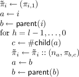
The proof that a data element d is stored at a certain position in the tree (and thereby in a certain position in the dataset) consists of a list of CVC-openings and intermediate nodes of the tree:

$$ \mathsf {\tilde{\pi }}_i = (\pi _l, n_l, \dots , n_1, \pi _0). $$

Here $\pi _l$ is an opening of the first component of $n_l$ to the element d, $\pi _{l-1}$ is an opening showing that the node $n_l$ is a child of node $n_{l-1}$, and eventually $\pi _0$ is an opening showing that node $n_1$ is a child of the root node. The whole proof $\mathsf {\tilde{\pi }}_i$ is called an authentication path.

To reduce the amount of data the client has to store, we exploit the key-features of our CVCs. Adding a new node to the tree requires knowledge of the parent of the new node, i.e., the value and the corresponding auxiliary information, but storing the entire tree at the client would defeat the purpose of a VDS protocol. To circumvent this problem, we make nodes recomputable. Namely, to create a new node $n_i$ for element $d_i$, we first derive the randomness $r_i$ of the CVC deterministically using a pseudorandom function, then compute the node $(n_i, \mathtt {aux}^*_i) \leftarrow \mathsf {CCom}_\mathtt {pp}(0, 0, \dots , 0; r_i)$ and find a collision $\mathtt {aux}_i \leftarrow \mathsf {CCol}_\mathtt {pp}(n_i, 1, 0, d, \mathtt {td}, \mathtt {aux}^*_i)$.

This idea allows us to split the tree between the client and the server in the following way: The client only stores the secret key $\mathsf {sp}= (k, \mathtt {td}, \texttt {cnt})$, whereas the server simply stores all data $d_1, d_2, \dots$ and all nodes $n_1, n_2, \dots$ along with their openings. Now, whenever the client wants to add a new data element d, it determines the next free index $i = \texttt {cnt}+ 1$ and the level l of the new node, as well as the index p of its parent and the position j this node will have in its parent. The client then computes the new node as $(n_i, \mathtt {aux}^*_i) \leftarrow \mathsf {CCom}_\mathtt {pp}(0, 0, \dots , 0; r_i)$, where the randomness $r_i$ is computed using the PRF. It adds the new data element by finding a collision for the first component $\mathtt {aux}_i \leftarrow \mathsf {CCol}_\mathtt {pp}(n_i, 1, 0, d, \mathtt {td}, \mathtt {aux}^*_i)$. With this, the client then can compute an opening of the first component of $n_i$, showing that d is indeed stored in $n_i$ in the first component: $\pi _l \leftarrow \mathsf {COpen}_\mathtt {pp}(1, d, \mathtt {aux}_i)$. To append this new node $n_i$ in the tree, the client recomputes the parent node as $(n_p, \mathtt {aux}^*_p) \leftarrow \mathsf {CCom}_\mathtt {pp}(0, 0, \dots , 0; r_p)$ and finds a collision in the j-th position: $\mathtt {aux}_p \leftarrow \mathsf {CCol}_\mathtt {pp}(n_p, j, 0, n_i, \mathtt {td}, \mathtt {aux}^*_p)$. From there, the client can then compute an opening of the parent node to the new node: $\pi _{l-1} \leftarrow \mathsf {COpen}_\mathtt {pp}(j, n_i, \mathtt {aux}_p)$. We call $(\pi _l, n_i, \pi _{l-1})$ an insertion path (since it is a partial authentication path). The client then sends the new data element and the insertion path $(d, (\pi _l,n_i, \pi _{l-1}))$ to the server, who stores this tuple in its database.

To answer a query on index i, the server computes a full authentication path for i by concatenating the insertion paths of all nodes on the path from i to the root. Note that each insertion path is of constant size due to the conciseness requirement for CVCs (see Definition 8), and thus the size of a full authentication path is only in $\mathcal {O}({\log _q{N}})$, where N is the number of elements in the dataset so far.

At first glance, the idea described so far seems to work. However, there is one more issue that needs to be overcome: The client may perform updates (i.e., change a data element from $d_i$ to $d'_i$) and continue appending new elements afterwards. This changes the value of $n_i$, and the client cannot recompute this value without storing all update-information. However, when appending a new child of $n_i$, the client has to find an opening of a position of this node $n_i$.

We solve this issue by letting the server store “an aggregate” of all update information. This way, the client can compute an “outdated” opening (i.e., as before any update) and then this opening can be updated by the server in constant time. Precisely, in the general case the server has to store a list of all updates and apply them one by one on incoming openings (in linear time). However, in the case of our CDH-based CVCs, we can exploit their homomorphic property to “accumulate” update-information by only storing its sum, thus achieving constant insertion time.

4.2 Formal Description of Our Construction

In this section, we present the formal description of our construction.

For better readability, we define the following three functions. The first one computes the index of the parent of node i, the second one computes in which component node i is stored in its parent, and the third function computes in which level of the tree node i can be found.

• $\mathsf {parent}(i) = \lfloor \frac{i-1}{q} \rfloor$

• $\mathsf {\#child}(i) = ((i-1) \mod q) + 2$

• $\mathsf {level}(i) = \lceil \log _q((q-1)(i+1)+1) - 1\rceil$

Construction 2

Let $\mathcal {CVC}= (\mathsf {CGen},\mathsf {CCom},\mathsf {COpen},\mathsf {CVer},\mathsf {CCol},\mathsf {CUpdate},\mathsf {CProofUpdate})$ be a CVC. Define $\mathcal {VDS}= (\mathsf {Setup},\mathsf{Append},{\mathsf{Query}},\mathsf{Verify},\mathsf{Update})$ as follows:

• $\mathsf {Setup}(1^{\lambda }, q){.}$ This algorithm picks a random PRF key $k \leftarrow \{0,1\}^{{\lambda }}$, computes a key-pair for the chameleon vector commitment $(\mathtt {pp}, \mathtt {td}) \leftarrow \mathsf {CGen}(1^{\lambda }, q+1)$, and sets the counter $\texttt {cnt}:= 0$. It computes $r_0 \leftarrow {\mathsf {f}}(k,0)$, sets the root as $(\rho , \mathtt {aux}_\rho ) \leftarrow \mathsf {CCom}_\mathtt {pp}(0, \dots , 0; r_0)$, the secret key $sk := (k,\mathtt {td},\texttt {cnt})$, and the public key $pk := (\mathtt {pp},\rho )$. Finally, the secret key $sk$ is kept by the client while the public key $pk$ is given to the server.

Before proceeding with the remaining algorithms, we summarize the information stored by the server. The server maintains a database DB consisting of tuples $(i, d_i, n_i, \pi _i, \pi _{p,j}, AU_i, \{AU_{i,j}\}_{j=1}^{q+1})$ where: $i \ge 0$ is an integer representing the index of every DB element, $d_i$ is DB value at index i, $n_i$ is a CVC commitment, $\pi _i$ is a CVC proof that $d_i$ is the first committed message in $n_i$, $\pi _{p,j}$ is a CVC proof that $n_i$ is the message at position $j+1$ committed in $n_p$ (which is the CVC of $n_i$’s parent node), $AU_i$ is the accumulated update information that can be used to update the proof $\pi _i$, and $AU_{i,j}$ are the accumulated update informations that can be used to update the children’s proofs $\pi _{i,j}$.

• $\mathsf{Append}( sk , d){.}$ The algorithm parses $sk = (k, \mathtt {td}, \texttt {cnt})$ and determines the index $i = \texttt {cnt}+ 1$ of the new element, the index $p = \mathsf {parent}(i)$ of its parent node, the position $j = \mathsf {\#child}(i)$ that this element will have in its parent, and then increases the counter $\texttt {cnt}' = \texttt {cnt}+ 1$. Next, it computes the new node as $(n_i, \mathtt {aux}^*_i) \leftarrow \mathsf {CCom}_\mathtt {pp}(0, 0, \dots , 0; r_i)$ where $r_i \leftarrow {\mathsf {f}}(k,i)$ and inserts the data d by finding a collision $\mathtt {aux}_i \leftarrow \mathsf {CCol}_\mathtt {pp}(n_i, 1, 0, d, \mathtt {td}, \mathtt {aux}^*_i)$. To append the node $n_i$ to the tree, the algorithm recomputes the parent node as $(n_p, \mathtt {aux}^*_p) \leftarrow \mathsf {CCom}_\mathtt {pp}(0, 0, \dots , 0; r_p)$ and inserts $n_i$ as the j-th child of $n_p$ by finding a collision in the parent node at position j, i.e., the client runs $\mathtt {aux}_p \leftarrow \mathsf {CCol}_\mathtt {pp}(n_p, j, 0, n_i, \mathtt {td}, \mathtt {aux}^*_p)$. It then computes $\pi _{i,1} \leftarrow \mathsf {COpen}_\mathtt {pp}(1, d, \mathtt {aux}_i)$ and $\pi _{p,j} \leftarrow \mathsf {COpen}_\mathtt {pp}(j, n_i, \mathtt {aux}_p)$, and sets the insertion path $(\pi _{i,1}, n_i, \pi _{p,j})$.

  The client $\mathcal {C}$ sends the above insertion path and the new element d to the server $\mathcal {S}$. $\mathcal {S}$ then applies the accumulated update $AU_{p,j}$ to $\pi _{p,j}$ (i.e., compute $\pi _{p,j}' \leftarrow \mathsf {CProofUpdate}'_\mathtt {pp}(\pi _{p,j}, AU_{p,j})$) and stores these items in its database DB.

• ${\mathsf{Query}}( pk , DB , i){.}$ In the query protocol, the client sends i to the server, who determines the level $l = \mathsf {level}(i)$ and constructs an authentication path:

  

  Finally, the server returns $\mathsf {\tilde{\pi }}_i$ to the client.

• $\mathsf{Verify}( pk , i, d, \mathsf {\tilde{\pi }}_i){.}$ This algorithm parses $pk = (\mathtt {pp}, \rho )$ and $\mathsf {\tilde{\pi }}_i = (\pi _l, n_l, \dots , n_1, \pi _0)$. It then proceeds by verifying all proofs in the authentication path:

  

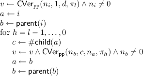
  If $v=1$ then output d. Otherwise output $\perp$.

• $\mathsf{Update}( pk , DB , sk , i, d'){.}$ In the update protocol, the client, given the secret key $sk$, sends an index i and a value $d'$ to the server. The server answers by sending the value d currently stored at position i and the corresponding authentication path $\mathsf {\tilde{\pi }}_i= (\pi _l, n_l, \dots , n_1, \pi _0)$ (this is generated as in the ${\mathsf{Query}}$ algorithm). The client then checks the correctness of $\mathsf {\tilde{\pi }}_i$ by running $\mathsf{Verify}( pk , i, d, \mathsf {\tilde{\pi }}_i)$. If the verification fails, the client stops running. Otherwise, it continues as follows. First, it parses $sk$ as $(k,\mathtt {td},\texttt {cnt})$, it determines the level of the updated node $l \leftarrow \mathsf {level}(i)$, and computes the new root $\rho '=n_0'$ as follows:

  

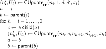
  On the other side, after receiving $(i, d')$, the server runs a similar algorithm to update all stored elements and proofs along the path of the new node. It also accumulates the new update information for every node in this path:

  

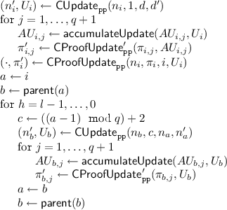
  In the above algorithms, a is the index of the changed node, b the index of its parent node, and c the position of node a in b. Basically, the algorithms change the value of node i, and then this change propagates up to the root ($\rho ' = n'_0$).

  Finally, both the client and the server compute the new public key as $pk = (\mathtt {pp}, \rho ')$.

4.3 Security

In this section, we show that the VDS protocol described in the previous section is secure.

Theorem 2

If ${\mathsf {f}}$ is a pseudorandom function and $\mathcal {CVC}$ is a secure CVC, then Construction 2 is a secure VDS.

Proof

We prove the theorem by first defining a hybrid game in which we replace the PRF with a random function. Such hybrid is computationally indistinguishable from the real $\mathsf {VDSsec}$ security game by assuming that ${\mathsf {f}}$ is pseudorandom. Then, we proceed to show that any efficient adversary cannot win with non-negligible probability in the hybrid experiment by assuming that the CVC scheme is secure. In what follows we use $Gm_{i,\mathcal {A}}({\lambda })$ to denote the experiment defined by Game i run with adversary $\mathcal {A}$.

• Game 0: this identical to the experiment $\mathsf {VDSsec}$.

• Game 1: this is the same as Game 0 except that the PRF ${\mathsf {f}}$ is replaced with a random function (via lazy sampling). It is straightforward to see that this game is negligibly close to Game 0 under the pseudo randomness of ${\mathsf {f}}$, i.e., ${\text {Prob }} \!\!\left[ Gm_{0,\mathcal {A}}({\lambda })=1\right] - {\text {Prob }} \!\!\left[ Gm_{1,\mathcal {A}}({\lambda })=1\right] = \mathsf {negl}({\lambda })$.

  Now, consider Game 1. Let $(i^*, d^*, \mathsf {\hat{\pi }})$ be the tuple returned by the adversary at the end of the game, d be the value currently stored in the database at index $i^*$. Recall that Game 1 outputs 1 if $\mathsf{Verify}( pk , i^*, d^*, \mathsf {\hat{\pi }})=1$ and $d \ne d^*$. Consider a honestly computed authentication path $\mathsf {\tilde{\pi }}$ for $(i^*, d)$ (this is the path which can be computed by the challenger), and observe that by construction the sequence in $\mathsf {\hat{\pi }}$ ends up at the public root. Intuitively, this means that $\mathsf {\hat{\pi }}$ and $\mathsf {\tilde{\pi }}$ must deviate at some point in the path from $i^*$ up to the root. We define $\mathsf{dcol}$ as the event that the two authentication paths deviate exactly in $i^*$, i.e., that $n_i = n^*_i$. Dually, if $\mathsf{dcol}$ does not occur, it intuitively means that the adversary managed to return a valid authentication path that deviates from a honestly computed one in some internal node. Clearly, we have:

  $$\begin{aligned} {\text {Prob }} \!\!\left[ Gm_{1,\mathcal {A}}({\lambda })=1\right]&= {\text {Prob }} \!\!\left[ Gm_{1,\mathcal {A}}({\lambda })=1 \wedge \mathsf {dcol}\right] \\&\qquad + {\text {Prob }} \!\!\left[ Gm_{1,\mathcal {A}}({\lambda })=1\wedge \overline{\mathsf {dcol}}\right] \end{aligned}$$

Our proof proceeds by showing that both

$$ {\text {Prob }} \!\!\left[ Gm_{1,\mathcal {A}}({\lambda })=1 \wedge \mathsf {dcol}\right] $$

and

$$ {\text {Prob }} \!\!\left[ Gm_{1,\mathcal {A}}({\lambda })=1\wedge \overline{\mathsf {dcol}}\right] $$

are negligible under the assumption that the CVC is position-binding.

${{Case}~{{{\textsf {\textit{dcol}}}}}}.$ In this case we build a reduction $\mathcal {B}$ against the position-binding property of the underlying CVC.

On input $\mathtt {pp}$, the reduction $\mathcal {B}$ computes the root node as described in the $\mathsf {catGen}$ algorithm, sets the counter $\texttt {cnt}:= 0$, and sets $pk \leftarrow (\mathtt {pp}, \rho )$. It then runs $\mathcal {A}(\mathsf {vp})$ by simulating the $\mathsf {VDSsec}$ game.

Whenever the adversary $\mathcal {A}$ streams some data element d, the reduction proceeds as described in the $\mathsf {catAdd}$ algorithm (except that pseudorandom values are now sampled randomly, as per Game 1). However, $\mathcal {B}$ does not know the full secret key $sk$ – it does not know the CVC trapdoor – but it can use its collision-oracle to compute the necessary collisions in the CVC in order to add new nodes to the tree. So, the reduction $\mathcal {B}$ returns $(i, \mathsf {\tilde{\pi }}_i)$ to the adversary and stores the tuple $(d, i, \mathsf {\tilde{\pi }}_i)$ in a list L.

Whenever the adversary $\mathcal {A}$ wants to update the element at position i to the new value $d'$, the reduction proceeds as described in the $\mathsf{Update}$ algorithm. Note that the CVC trapdoor is not needed in this phase. $\mathcal {B}$ then returns the updated proof $\mathsf {\tilde{\pi }}'_i$ to $\mathcal {A}$ and updates the tuple $(d', i, \mathsf {\tilde{\pi }}'_i)$ in L.

Eventually the adversary outputs $(d^*, i^*, \mathsf {\hat{\pi }}^*)$. The reduction then finds the actual data d and the corresponding proof $\mathsf {\tilde{\pi }}_i$ for position i by searching for the tuple $(d, i^*, \mathsf {\tilde{\pi }}_i)$ in L, parses $\mathsf {\hat{\pi }}^* = (\pi ^*, n^*_i, \dots )$ and $\mathsf {\tilde{\pi }}_i = (\pi , n_i, \dots )$ and outputs $(n_i, 1, d, d^*, \pi , \pi ^*)$.

For the analysis now observe that $\mathcal {B}$ is efficient as so is $\mathcal {A}$, and searching for a tuple in an ordered list can be done in polynomial time. It is easy to see that $\mathcal {B}$ perfectly simulates the view for $\mathcal {A}$ as in the game $\mathsf {VDSsec}$. Now, whenever $\mathsf {dcol}$ happens, we know that $n^*_i = n_i$. Hence both $(\pi , d)$ and $(\pi ^*, d^*)$ must verify correctly whenever $\mathcal {A}$ wins. Furthermore, observe that $\mathcal {B}$ never uses its collision-oracle on position 1, since the $\mathsf{Append}$ algorithm always uses $\mathsf {CCol}$ on index $j > 1$. This means essentially means that

$$\begin{aligned} {\text {Prob }} \!\!\left[ Gm_{1,\mathcal {A}}({\lambda })=1 \wedge \mathsf {dcol}\right]&\le {\text {Prob }} \!\!\left[ \mathsf {PosBdg}_\mathcal {B}({\lambda }, q) = 1\right] \\&\qquad = \mathsf {negl}({\lambda }) \end{aligned}$$

$Case \,{\overline{{{\textsf {\textit{dcol}}}}}}$ Recall that in this case Game 1 outputs 1 only if the adversary wins by returning an authentication path which deviates from the correct one at some internal node in the path from $i^{*}$ up to the root. In this case too, we build a reduction $\mathcal {B}$ against the position-binding property of the underlying CVC.

On input $\mathtt {pp}$, the reduction $\mathcal {B}$. It then tries to set an upper limit on the number of elements the adversary will authenticate in the tree by choosing its depth $l = {\lambda }$. The reduction then builds a tree of CVCs of size l from bottom to top, where in each CVC every position which does not point to a child (especially the first position) is set to 0. Denote the root of this tree by $\rho$. Finally, the reduction $\mathcal {B}$ sets $\texttt {cnt}:= 0$, sets $pk \leftarrow (\mathtt {pp}, \rho )$ and runs $\mathcal {A}( pk )$ by simulating Game 1 to it.

Whenever the adversary $\mathcal {A}$ streams some data element d to the reduction, the reduction determines the index $i = \texttt {cnt}+ 1$ for the new data element, increases $\texttt {cnt}$ by one and inserts the new element into the tree by finding a collision in the first component of node $n_i$ using its collision-oracle. It then computes an authentication path $\mathsf {\tilde{\pi }}_i$ for d as described in the $\mathsf{Append}$ algorithm. The reduction returns $(i, \mathsf {\tilde{\pi }}_i)$ to the adversary and stores $(d, i, \mathsf {\tilde{\pi }}_i)$ in some list L. If the adversary exceeds the number of elements l, the reduction stops the adversary $\mathcal {A}$, increases $l \leftarrow l \cdot {\lambda }$, and starts again.

Whenever the adversary $\mathcal {A}$ wants to update the element at position i to some new value $d'$ the reduction proceeds as described in the $\mathsf{Update}$ algorithm. It then returns the updated proof $\mathsf {\tilde{\pi }}'_i$ to the adversary and updates the tuple $(d', i, \mathsf {\tilde{\pi }}'_i)$ in L.

At the end of the game the adversary outputs $(d^*, i^*, \mathsf {\hat{\pi }}^*)$. The reduction parses $\mathsf {\hat{\pi }}^* = (\pi ^*_0, n^*_0, \pi ^*_1, \dots )$ and finds the largest j for which $n^*_i = n_j$, i.e., for which the authentication path $\mathsf {\hat{\pi }}^*$ still agrees with the actual tree. Also $\mathcal {B}$ finds the authentication path $\mathsf {\tilde{\pi }}_{i^*} = (\pi ^{i^*}_0, n^{i^*}_0, \pi ^{i^*}_1, \dots )$ up to $i^*$, if $i^{*}$ was streamed by the adversary, or otherwise up to the deepest ancestor of $i^{*}$. Clearly, $\pi ^*_i$ then must be a proof that $n^*_{i-1}$ is “stored” in $n^*_i$ at some position h.

If $n_j$ is the deepest node in the path towards $i^{*}$ that is stored by the challenger then the h-th message committed in $n_j$ by the challenger is 0. In this case $\mathcal {B}$ can produce a honest proof $\pi _{h,0}$ that 0 is the h-th message committed in $n_j$, and then outputs $(n_j, h, 0, n^*_{i-1}, \pi _{h,0}, \pi ^*_i)$.

Otherwise, if $n_j$ is not the deepest node, the honest path $\mathsf {\tilde{\pi }}_{i^*}$ must contain a node $n^{i^*}_k = n_j$ as well as a proof $\pi ^{i^*}_k$ that the node $n^{i^*}_{k-1}$ is the h-th child of $n_j$. In this case $\mathcal {B}$ outputs $(n_j, h, n^{i^*}_{k-1}, n^*_{i-1}, \pi ^{i^*}_k, \pi ^*_i)$. As one can check, this case also captures the on in which $h=1$ and $n^{i^*}_{k-1} = d \ne d^{*} = n^*_{i-1}$.

For the analysis see that $\mathcal {B}$ is efficient because $\mathcal {A}$ is and because the limit l will be large enough after a polynomial number of times. Now observe that $\mathcal {B}$ perfectly simulates the view of $\mathcal {A}$ in Game 1 (otherwise the underlying CVC would not have indistinguishable collisions). It is easy to see that whenever $\mathcal {A}$ wins the pair $(\pi ^*_i, n^*_{i-1})$ verifies w.r.t. $n_j$. As $\mathcal {B}$ honestly computed $n^{i^*}_{k-1}$ and $\pi ^{i^*}_k$, this pair will also verify w.r.t. $n_j$. Note that $\mathcal {B}$ only asks for collisions at position 1, but $h > 1$. Therefore $\mathcal {B}$ wins whenever $\mathcal {A}$ does. Since the underlying CVC is position-binding, this probability is at most negligible.

$$\begin{aligned} {\text {Prob }} \!\!\left[ Gm_{1,\mathcal {A}}({\lambda })=1 \wedge \overline{\mathsf {dcol}}\right]&\le {\text {Prob }} \!\!\left[ \mathsf {PosBdg}_\mathcal {B}({\lambda }, q) = 1\right] \\&\qquad = \mathsf {negl}({\lambda }) \end{aligned}$$

Since both parts are at most negligible in ${\lambda }$, the overall success probability of any efficient adversary can only be negligible in ${\lambda }$, hence Construction 2 is secure according to Definition 6.

4.4 Reducing the Public Key Size

Instantiating the scheme from Construction 2 with the CVCs from Construction 1 results in a public key of size $\mathcal {O}({q^2})$ due to the values $h_{i,j}$ that are stored in the public parameters $\mathtt {pp}$, which are part of the VDS public key. As an interesting extension, we show how to reduce the public key size of our VDS protocol to $\mathcal {O}({1})$ by carefully inspecting our usage of the CVC scheme from Construction 1. In particular, note that the public key of the VDS protocol consists of: elements that are required for public verifiability of queried data elements, and elements only needed by the server.

The elements $h_{i,j}$ are only needed for $\mathsf {COpen}$ in the $\mathsf{Append}$ protocol on the client-side, and in $\mathsf {CProofUpdate}$ in the $\mathsf{Update}$ protocol on the server-side. They are, however, not used for public verifiability in the VDS protocol. Therefore, these values $h_{i,j}$ do not need to be part of the public verification key of the VDS protocol, and can be sent directly to the server only once. This already reduces the key size from $\mathcal {O}({q^{2}})$ to $\mathcal {O}({q})$.

To get rid of the remaining elements $h_1,\dots ,h_q$ in the public key, we observe that during each run of $\mathsf{Verify}$, only one of these $h_i$ values is needed at every level. This allows us to do the following change to the protocol: Instead of storing all $h_1, \dots , h_q$ in the public key, we let the client sign each $h_i$, together with its index i, using a regular signature scheme. For every i one thus obtain a signature $\sigma _i$, and the server is required to store all pairs $(h_1, \sigma _1), \dots , (h_q, \sigma _q)$. Later when the server has to provide the answer to a query, we require it to include all the necessary $(h_i, \sigma _i)$ pairs in the authentication path. Note that these pairs are most q, and thus do not increase the asymptotic length of the authentication path. The verifier will eventually verify that $\sigma _i$ is a valid signature on $h_i || i$, before using $h_i$ in $\mathsf {CVer}$. This change allows us to replace the q $h_i$ values from the public key with a single verification key of a signature scheme, and it results in a VDS protocol with a public key size of size $\mathcal {O}({1})$.

5 VDS from Accumulators

Our second construction is conceptually very different from all previous VDS constructions, since it does not rely on any tree structure. The basic idea is to let the client sign each element of the dataset with a regular signature scheme, and to use a cryptographic accumulator to revoke old signatures once an element gets updated (otherwise the server could perform a rollback attack). For this, the client has a key-pair of a signature scheme, and his public key serves as the public verification key. Whenever an element is queried from the server, the server return the element, its signature, and a proof-of-non-membership, to show that this signature has not been revoked yet.

However, this idea does not work immediately. One reason is that some accumulators only support the accumulation of an a priori fixed number of elements such as [15]. Another issue is that the size of the public-key is typically linear in the number of accumulated values, and thus the client might not be able to store it.

In our construction we solve this issue by exploiting the specific algebraic properties of the bilinear-map accumulator as follows: The bilinear-map accumulator [15] and its extension to support non-membership proofs [7] use a private key s and a public key $g, g^s, \dots , g^{s^q}$, where q is an upper bound on the number of elements in the accumulator. To compute a proof of (non-)membership for q accumulated elements, all the values $g, g^s, \dots , g^{s^q}$ are needed. However, to verify a proof of (non-)membership only the values g and $g^s$ is required. In our VDS scheme, we only require that proofs of non-membership can be verified publicly; they do not need to be publicly computable with only the public key and the accumulator value. Therefore we only put g and $g^s$ into our public key. Only the client has to add additional items to the accumulator, but he can do so using his private key s and g to recompute $g^s, \dots , g^{s^q}$. Furthermore, only the server has to compute proofs of non-membership and thus needs to know $g, g^s, \dots , g^{s^q}$, where q is the number of updates so far. Since we do not want to fix an upper bound on the number of updates a priori, the client extends the list of known values of the server with each update-operation. E.g. in the update protocol for the third element the client sends the value $g^{s^3}$ to the server who then appends this value to a list.

This allows us to reduce the size of the public-key to $\mathcal {O}({1})$, and to support an unbounded number of updates.

5.1 Our Scheme

In this section we show how to use the bilinear-map accumulator described in Sect. 2.5 in combination with a signature scheme to build a VDS protocol.

Construction 3

Let $\mathsf {Sig}=(\mathsf {SKg},\mathsf {Sign},\mathsf {Vrfy})$ be a signature scheme and ${H:\{0,1\}^* \mapsto \mathbb {Z}_p^*}$ be a hash function. The VDS protocol $\mathcal {VDS}=(\mathsf {Setup},\mathsf{Append},{\mathsf{Query}},\mathsf{Verify},\mathsf{Update})$ is defined as follows:

• $\mathsf {Setup}(1^{\lambda }){.}$ The setup algorithm first generates a tuple of bilinear map parameters $(p,\mathbb {G},{\mathbb {G}_T},e,g)$. Second, it chooses s at random from $\mathbb {Z}_p^*$ and computes $g^s$. Next, it generates a key-pair $( ssk , vk )\leftarrow \mathsf {SKg}(1^{\lambda })$, initializes two counters $\texttt {cnt}:=0$ and $\mathtt {upd}:=0$, and sets $S_{last} = g$. It also generates an initially empty accumulator $f'(\mathcal {E}):=g$. Note that during the lifetime of the scheme, the server will increasingly store $g, g^s, \ldots , g^{s^{\mathtt {upd}}}$ while the client only stores $S_{last}=g^{s^{\mathtt {upd}}}$. Finally, the algorithm outputs the secret key $sk =(g,p,s, ssk , S_{last}, \texttt {cnt}, \mathtt {upd})$ which is kept by the client, and the public key $pk =(p,\mathbb {G},{\mathbb {G}_T},e,g,g^s, vk ,f'(\mathcal {E}))$ which is given to the server.

• $\mathsf{Append}( sk , d){.}$ The append algorithm increases the counter $\texttt {cnt}:=\texttt {cnt}+1$, chooses a random tag $\mathtt {tag}\leftarrow \{0,1\}^{\lambda }$, and signs the value $m:=d\Vert \mathtt {tag}\Vert \texttt {cnt}$ by computing $\sigma \leftarrow \mathsf {Sign}( ssk ,m)$. The pair $((d,\mathtt {tag},\texttt {cnt}),\sigma )$ is finally sent to $\mathcal {S}$, who stores it at position $\texttt {cnt}$ in $DB$.

• ${\mathsf{Query}}( pk , DB , i){.}$ To retrieve the i-th element from $DB$, the client sends i to $\mathcal {S}$, who computes the response as follows: $\mathcal {S}$ retrieves the pair $(m,\sigma )$ from $DB$ and computes a proof of non-membership (w, u) for the element $e_i \leftarrow H(\sigma )$ as described in Sect. 2.5. Finally, $\mathcal {S}$ returns $(d,\pi )=((d',\mathtt {tag},i),(\sigma ,w,u))$.

• $\mathsf{Verify}( pk , i, d, \pi ){.}$ This algorithm parses $pk =(p,\mathbb {G},{\mathbb {G}_T},e,g,g^s, vk ,f'(\mathcal {E}))$, $d=(d',\mathtt {tag},i)$, and $\pi =(\sigma ,w,u)$. It sets $e_i\leftarrow H(\sigma )$, and outputs $d'$ iff $\mathsf {Vrfy}( vk , d'||\mathtt {tag}||i, \sigma )=1$ and $e(w,g^{e_i}\cdot g^s) = e( f'(\mathcal {E}) \cdot g^u,g)$.

• $\mathsf{Update}( sk , DB , sk , i, d'){.}$ The clients runs $(d,\pi ) \leftarrow {\mathsf{Query}}( pk , DB , i)$ to retrieve the i-th entry from $DB$. Afterwards, $\mathcal {C}$ verifies the correctness of the entry by running the verification algorithm $\mathsf{Verify}( pk , i, d, \pi )$. If $\mathsf{Verify}$ outputs 1, then $\mathcal {C}$ increases the counter $\mathtt {upd}:=\mathtt {upd}+1$, signs the new element $\sigma ' \leftarrow \mathsf {Sign}( ssk ,d'||\mathtt {tag}||i)$ using a random tag $\mathtt {tag}\leftarrow \{0,1\}^{\lambda }$, and adds the old signature to the accumulator as follows. The client computes $g^{s^\mathtt {upd}} = S_{last} := (S_{last})^s$, $e_i\leftarrow H(\sigma )$, and $f''(\mathcal {E}):=f'(\mathcal {E})^{e_i+s}$. The client sends $(g^{s^\mathtt {upd}},f''(\mathcal {E}),\sigma ')$ to $\mathcal {S}$. The server stores $(\sigma ',d')$ at position i in $DB$, and $g^{s^\mathtt {upd}}$ in its parameters. The public key is then updated to $pk ':=(p,\mathbb {G},{\mathbb {G}_T}, e, g, g^s, vk , f''(\mathcal {E}))$.

Theorem 3

If $\mathsf {Sig}$ is a strongly unforgeable signature scheme, H a collision-resistant hash function, and $\mathsf {ACC}$ the collision-resistant accumulator as defined in Sect. 2.5, then  Construction 3 is a secure VDS protocol.

Proof

Let $\mathcal {A}$ be an efficient adversary against the security of Construction 3 as defined in game $\mathsf {VDSsec}$, denote by $pk ^*:=(p,\mathbb {G},{\mathbb {G}_T},e_i,g,g^s, vk ,f^*(\mathcal {E}))$ the public-key hold by the challenger at the end of the game, and let

$$ Q:=((d_1||\mathtt {tag}_1 || 1, \sigma _1), (d_2|| \mathtt {tag}_2 || 2, \sigma _2),\dots ,(d_n|| \mathtt {tag}_n || n,\sigma _n)) $$

be the state of the database $DB$ at the end of the game. By $(w_1,u_1),\dots ,(w_n,u_n)$ we denote the witnesses of the non-membership proofs that be can be computed by the challenger using public values only, as discussed in Sect. 2.5, and denote by $Q':=((d'_1||\mathtt {tag}'_1 || i_1', \sigma _1'), (d'_2|| \mathtt {tag}'_2 || i_2', \sigma '_2),\dots ,(d'_n|| \mathtt {tag}'_n || i_n ,\sigma '_n))$ all queries sent by $\mathcal {A}$. Clearly, $Q \subseteq Q'$ and let $O := Q' \backslash Q$ be the set of queries that have been sent by the adversary and which are not in the current database. Let $\mathcal {A}$ be an efficient adversary that outputs $((d^*,\mathtt {tag}^*,i^*),(\sigma ^*,w^*,u^*))$ such that $(\hat{d}, i^*) \not \in Q$, $\mathsf {Vrfy}( vk , d^*||\mathtt {tag}^*||i^*,\sigma )=1$, and $e(w^*,g^{e^*_i}\cdot g^s) = e( f'(\mathcal {E}) \cdot g^{u^*},g)$, with $e^*_i :=H(\sigma ^*)$. Then, we define the following events:

• $\mathsf {hcol}$ is the event that there exists an index $1\le i \le n$ such that $H(\sigma ^*)=H(\sigma '_i)$ and $\sigma ^* \ne \sigma '_i$.

• $\mathsf {fake}$ is the event that $e(w^*,g^{e^*_i}\cdot g^s) = e( f'(\mathcal {E}) \cdot g^{u^*},g)$ and $e_i \in \mathcal {E}$.

Observe that the case where the adversary finds a collision in the accumulator and the one where he finds a fake witness for a membership of a non-member of $\mathcal {E}$, do not help to break the security of the VDS scheme. Given these events, we can bound $\mathcal {A}$’s success probability as follows:

$$\begin{aligned}&{\text {Prob }} \!\!\left[ \mathsf {VDSsec}^\mathcal {VDS}_\mathcal {A}({\lambda })=1\right] \le {\text {Prob }} \!\!\left[ \mathsf {hcol}\right] + {\text {Prob }} \!\!\left[ \mathsf {fake}\right] +\\&\qquad \qquad \qquad {\text {Prob }} \!\!\left[ \mathsf {VDSsec}^\mathcal {VDS}_\mathcal {A}({\lambda })=1 \;\wedge \; \overline{\mathsf {hcol}}\;\wedge \; \overline{\mathsf {fake}}\right] \end{aligned}$$

In the following we show that the parts of the sum are negligible. The fact that ${\text {Prob }} \!\!\left[ \mathsf {hcol}\right]$ is negligible, follows trivially by the collision-resistance of the hash function. Furthermore, it is also easy to see that ${\text {Prob }} \!\!\left[ \mathsf {fake}\right]$ is negligible as well due to proof of non-membership properties of the accumulator.

Claim

${\text {Prob }} \!\!\left[ \mathsf {VDSsec}^\mathcal {VDS}_\mathcal {A}({\lambda })=1\wedge \overline{\mathsf {hcol}}\wedge \overline{\mathsf {fake}}\right] \approx 0$.

This claim follows from the strong unforgeability of the underlying signature scheme. The intuition is that the correct proof non-membership guarantees that the signature is not stored in the accumulator. Since it is not stored in the accumulator, the adversary did not receive this signature from the signing oracle and thus, is a valid forger w.r.t. strong unforgeability.

More formally, let $\mathcal {A}$ be an efficient adversary against the security of the VDS protocol. Then we construct an algorithm $\mathcal {B}$ against the strong unforgeability as follows. The input of $\mathcal {B}$ is a public-key $vk$ and it has access to a signing oracle. It generates random elements $(p,\mathbb {G},{\mathbb {G}_T},e,g,g^s)$ for some s chosen at random from $\mathbb {Z}_p^*$, counters $\texttt {cnt}:=0$ and $\mathtt {upd}:=0$, and $\mathcal {B}$ also generates an initially empty accumulator $f'(\mathcal {E}):=g$. It runs $\mathcal {A}$ on $pk =(p,\mathbb {G},{\mathbb {G}_T},e,g,g^s, vk ,f'(\mathcal {E}))$ in a black-box way. Whenever $\mathcal {A}$ wishes to append an element d, then $\mathcal {B}$ increments the counter $\texttt {cnt}:=\texttt {cnt}+1$, chooses a fresh tag $\mathtt {tag}$, sends $m':=d||\mathtt {tag}||\texttt {cnt}$ to its signing oracle and forwards the response $\sigma$ together with the corresponding proof of non-membership to $\mathcal {A}$.

It is understood that $\mathcal {B}$ records all s queries and answers. If $\mathcal {A}$ wants to update the ith element, then $\mathcal {B}$ adds the corresponding signature $\sigma _i$ to the accumulator, increases the counter $\mathtt {upd}:=\mathtt {upd}+1$, picks a fresh tag $\mathtt {tag}'$ at random, sends $m':=d'||\mathtt {tag}'||\texttt {cnt}$ to its singing oracle and forwards the response together with a proof of non-membership and $g^{s^{\mathtt {upd}}}$ to $\mathcal {A}$. Eventually, $\mathcal {A}$ stops, outputting $((d^*,\mathtt {tag}^*,i^*),(\sigma ^*,w^*,u^*))$. The algorithm $\mathcal {B}$ then outputs $((d^*||\mathtt {tag}^*||i^*),\sigma ^*)$.

For the analysis, it’s easy to see that $\mathcal {B}$ is efficient and performs a perfect simulation from $\mathcal {A}$’s point of view. In the following, let’s assume that $\mathcal {B}$ succeeds with non-negligible probability, i.e., $((d^*,\mathtt {tag}^*,i^*),(\sigma ^*,w^*,u^*))$ satisfies the following: $(\hat{d}, i^*) \not \in Q$, $\mathsf {Vrfy}( vk , d^*||\mathtt {tag}^*||i^*,\sigma )=1$, and $e(w^*,g^{e^*_i}\cdot g^s) = e( f'(\mathcal {E}) \cdot g^{u^*},g)$, with $e^*_i :=H(\sigma ^*)$. We now argue, that $\mathcal {B}$ succeeds whenever $\mathcal {A}$ does. To see this observe that $(\hat{d}, i^*) \not \in Q$ and that the proof of non-membership verifies. Thus, conditioning on $\overline{\mathsf {fake}}$ and on $\overline{\mathsf {hcol}}$ the claim follows.

6 Experimental Results

We implemented the construction based on chameleon vector commitments (Sect. 4) and on accumulators (Sect. 5) in Java 1.7.

In this section, we provide comprehensive benchmarks of all proposed schemes to evaluate their practicality. We investigate the computational and bandwidth overhead induced by our protocols. We use the PBC library [11] in combination with a java wrapper for pairing-based cryptographic primitives (using a type D-201 MNT curve), and the Bouncy Castle Cryptographic API 1.50 [3] for all other primitives. For the construction based on accumulators, we used RSA-PSS with 1024 bit long keys as our underlying signature scheme, and SHA-1 as our hash function. Our experiments were performed on an Amazon EC2 r3.large instance equipped with 2 vCPU Intel Xeon Ivy Bridge processors, 15 GiB of RAM and 32 GB of SSD storage running Ubuntu Server 14.04 LTS (Image ID ami-0307d674).

We stress that this is an unoptimized, prototype implementation, and that better performance results may be achieved by further optimizations.

${\underline{\textsc {Dataset:}}}$ We evaluated our schemes by outsourcing and then retrieving 8 GB, using chunk-sizes of 256 kB, 1 MB, and 4 MB. We measured the insertion and the verification time on the client side, as well as the sizes of all transmitted proofs.

${\underline{\textsc {Branching\;Factor:}}}$ The CVC-based VDS was instantiated with branching factors of $q=32,64,128$, and 256, and the public-key consists of $q^2$ elements that amount to 2.7 MB (for $q=256$). This is in contrast to the public key size in the accumulator-based VDS which is about 350 bytes.

${\underline{\textsc {Number\;of\;Updates:}}}$ To quantify the impact of updates on the accumulator-based construction, we performed separate experimental runs. Therefore, we performed 0, 10, 50 and 100 updates prior to retrieving and verifying the outsourced data set.

${\underline{\textsc {Block\;Sizes:}}}$ The block size is a parameter which depends heavily on the application. Larger block sizes reduce the number of authenticated blocks, and thus yield a smaller tree with more efficient bandwidth and computation performance in the CVC-based VDS. However, larger blocks decrease the granularity of on-the-fly verification, since one has to retrieve an entire block prior to verification.

We took measurements for block sizes of 256 kB, 1 MB and 4 MB, which we believe is a sensible range of block sizes for various applications. For example, consider HD-video streaming with a bandwidth of 8 MB/s. Using a block size of 4 MB means that one can perform a verification every 0.5 s. However, in other applications such as the verifiable stock market, one may want to only retrieve a small fraction of the outsourced data set, for which a smaller block size such as 256 kB might be more desirable.

Fig. 2.

Average insertion time for different block sizes (Color figure online)

6.1 Streaming Data

Both proposed constructions have constant client-side insertion times as well as constant bandwidth overheads. The insertion proofs in the accumulator-based and the CVC-based construction are 236 respectively 1070 bytes large. Rather than processing each block directly, we first compute its hash value and pass it to our VDS protocol. Since the insertion time is dominated by this hash function, we give the average insertion times for our different block sizes in Fig. 2. As one can see, the accumulator-based construction performs slightly better than the CVC-based one, and both give rise to quite practical timings for the insertion phase.

Fig. 3.

Accumulated verification time for retrieving 8 GB (Color figure online)

Fig. 4.

Accumulated bandwidth overhead for retrieving 8 GB (Color figure online)

6.2 Verifying Retrieved Elements

The time needed for verifying the correctness of 8 GB data retrieved from the server is depicted in Fig. 3. In this figure, various insights about the performance behavior of our protocols are visible.

Firstly, the block size plays a crucial role for the overall performance, since the number of verifications needed to authenticate the 8 GB dataset depends linearly on the inverse of the block size.

Secondly, in the CVC-based construction higher tree arity results in shorter proofs, and therefore faster verification.

Thirdly, we observe the impact of updates on our accumulator-based construction. While without updates the accumulator-based construction is faster than the CVC-based one, adding just 10 updates decreases the performance of the accumulator dramatically. Still, for applications where only a few updates are expected, our accumulator-based construction is preferable.

6.3 Bandwidth Overhead

The bandwidth overhead incurred by retrieving 8 GB of data is shown in Fig. 4. As in Fig. 3 the impact of the block size is visible, as is the impact of the branching factor of the CVC-based construction. This figure also shows that the accumulator-based construction, although slower when handling updates, achieves a much smaller bandwidth overhead compared to the CVC-based construction. However, in this scenario for a block-size of 4 MB, both constructions introduce a total bandwidth overhead of less than 4 MB, or $0.05\,\%$.

References

Bao, F., Deng, R.H., Zhu, H.: Variations of Diffie-Hellman problem. In: Qing, S., Gollmann, D., Zhou, J. (eds.) ICICS 2003. LNCS, vol. 2836, pp. 301–312. Springer, Heidelberg (2003)
Benabbas, S., Gennaro, R., Vahlis, Y.: Verifiable delegation of computation over large datasets. In: Rogaway, P. (ed.) CRYPTO 2011. LNCS, vol. 6841, pp. 111–131. Springer, Heidelberg (2011)
Castle, B.: The Legion of the Bouncy Castle. https://www.bouncycastle.org
Camenisch, J., Kohlweiss, M., Soriente, C.: An accumulator based on bilinear maps and efficient revocation for anonymous credentials. In: Jarecki, S., Tsudik, G. (eds.) PKC 2009. LNCS, vol. 5443, pp. 481–500. Springer, Heidelberg (2009)
Camenisch, J.L., Lysyanskaya, A.: Dynamic accumulators and application to efficient revocation of anonymous credentials. In: Yung, M. (ed.) CRYPTO 2002. LNCS, vol. 2442, pp. 61–76. Springer, Heidelberg (2002)
Catalano, D., Fiore, D.: Vector commitments and their applications. In: Kurosawa, K., Hanaoka, G. (eds.) PKC 2013. LNCS, vol. 7778, pp. 55–72. Springer, Heidelberg (2013)
Damgård, I., Triandopoulos, N.: Supporting non-membership proofs with bilinear-map accumulators. Cryptology ePrint Archive, Report 2008/538 (2008). http://eprint.iacr.org/2008/538
Krawczyk, H., Rabin, T.: Chameleon signatures. In: ISOC Network and Distributed System Security Symposium - NDSS 2000. The Internet Society, February 2000
Krupp, J., Schröder, D., Simkin, M., Fiore, D., Ateniese, G., Nuernberger, S.: Nearly optimal verifiable data streaming (full version). Cryptology ePrint Archive, Report 2015/333 (2015). http://eprint.iacr.org/2015/333
Libert, B., Yung, M.: Concise mercurial vector commitments and independent zero-knowledge sets with short proofs. In: Micciancio, D. (ed.) TCC 2010. LNCS, vol. 5978, pp. 499–517. Springer, Heidelberg (2010)
Lynn, B.: PBC - C Library for Pairing Based Cryptography. http://crypto.stanford.edu/pbc/
Martel, C., Nuckolls, G., Devanbu, P., Gertz, M., Kwong, A., Stubblebine, S.G.: A general model for authenticated data structures. Algorithmica 39, 2004 (2001)
Maurer, U.M., Wolf, S.: Diffie-Hellman oracles. In: Koblitz, N. (ed.) CRYPTO 1996. LNCS, vol. 1109, pp. 268–282. Springer, Heidelberg (1996)
Naor, M., Nissim, K.: Certificate revocation and certificate update. IEEE J. Sel. Areas Commun. 18(4), 561–570 (2000)
Nguyen, L.: Accumulators from bilinear pairings and applications. In: Menezes, A. (ed.) CT-RSA 2005. LNCS, vol. 3376, pp. 275–292. Springer, Heidelberg (2005)
Papamanthou, C., Shi, E., Tamassia, R., Yi, K.: Streaming authenticated data structures. In: Johansson, T., Nguyen, P.Q. (eds.) EUROCRYPT 2013. LNCS, vol. 7881, pp. 353–370. Springer, Heidelberg (2013)
Papamanthou, C., Tamassia, R.: Time and space efficient algorithms for two-party authenticated data structures. In: Qing, S., Imai, H., Wang, G. (eds.) ICICS 2007. LNCS, vol. 4861, pp. 1–15. Springer, Heidelberg (2007)
Perrig, A., Canetti, R., Song, D., Tygar, J.D.: Efficient and secure source authentication for multicast. In: ISOC Network and Distributed System Security Symposium - NDSS 2001, pp. 35–46. The Internet Society, February 2001
Perrig, A., Canetti, R., Tygar, J.D., Song, D.X.: Efficient authentication and signing of multicast streams over lossy channels. In: 2000 IEEE Symposium on Security and Privacy, pp. 56–73. IEEE Computer Society Press, May 2000
Ruffing, T., Kate, A., Schröder, D.: Liar, liar, coins on fire!: penalizing equivocation by loss of bitcoins. In: Proceedings of the 22nd ACM SIGSAC Conference on Computer and Communications Security, Denver, CO, USA, 12–6 October 2015, pp. 219–230. ACM (2015)
Schröder, D., Schröder, H.: Verifiable data streaming. In: Yu, T., Danezis, G., Gligor, V.D. (eds.) 19th Conference on Computer and Communications Security, ACM CCS 2012, pp. 953–964. ACM Press, October 2012
Schöder, D., Simkin, M.: VeriStream – a framework for verifiable data streaming. In: Böhme, R., Okamoto, T. (eds.) FC 2015. LNCS, vol. 8975, pp. 548–566. Springer, Heidelberg (2015)
Stefanov, E., van Dijk, M., Juels, A., Oprea, A.: Iris: a scalable cloud file system with efficient integrity checks. In: Proceedings of the 28th Annual Computer Security Applications Conference, ACSAC 2012, pp. 229–238. ACM, New York (2012)
Tamassia, R., Triandopoulos, N.: Certification and authentication of data structures. In: AMW (2010)
Acknowledgments
This work was supported by the German Federal Ministry of Education and Research (BMBF) through funding for the Center for IT-Security, Privacy and Accountability (CISPA – www.cispa-security.org) and the project PROMISE. Moreover, it was supported by the Initiative for Excellence of the German federal and state governments through funding for the Saarbrücken Graduate School of Computer Science and the DFG MMCI Cluster of Excellence. Part of this work was also supported by the German research foundation (DFG) through funding for the collaborative research center 1223. Dominique Schröder was also supported by an Intel Early Career Faculty Honor Program Award.
Author information
Authors and Affiliations
Corresponding author
Editor information
Editors and Affiliations
Rights and permissions
Copyright information
© 2016 International Association for Cryptologic Research
About this paper
Cite this paper
Krupp, J., Schröder, D., Simkin, M., Fiore, D., Ateniese, G., Nuernberger, S. (2016). Nearly Optimal Verifiable Data Streaming. In: Cheng, CM., Chung, KM., Persiano, G., Yang, BY. (eds) Public-Key Cryptography – PKC 2016. Lecture Notes in Computer Science(), vol 9614. Springer, Berlin, Heidelberg. https://doi.org/10.1007/978-3-662-49384-7_16
Download citation
DOI: https://doi.org/10.1007/978-3-662-49384-7_16
Published:
Publisher Name: Springer, Berlin, Heidelberg
Print ISBN: 978-3-662-49383-0
Online ISBN: 978-3-662-49384-7
eBook Packages: Computer ScienceComputer Science (R0)