Highway Travel Time Measurement from Toll Ticket Data

Abstract

Travel time for a road trip is a drivers’ most appreciated traffic information. Measuring travel times on a real time basis is also a perfect indicator of the level of service in a road link, and therefore is a useful measurement for traffic managers in order to improve traffic operations on the network. In conclusion, accurate travel time measurement is one of the key factors in traffic management systems. This chapter presents a new approach for measuring travel times on closed toll highways using the existing surveillance infrastructure. In a closed toll system, where toll plazas are located on the on/off ramps and each vehicle is charged a particular fee depending on its origin and destination, the data used for toll collection can also be valuable for measuring mainline travel times on the highway. The proposed method allows estimating mainline travel times on single sections of highway (defined as a section between two neighboring ramps) using itineraries covering different origin–destinations. The method provides trip time estimations without investing in any kind of infrastructure or technology. This overcomes some of the limitations of other methods, like the information delay and the excess in the travel time estimation due to the accumulation of exit times (i.e. the time required to travel along the exit link plus the time required to pay the fee at the toll gate). The results obtained in a pilot test on the AP-7 toll highway, near Barcelona in Spain, show that the developed methodology is sound.

Appendices

Appendix 5A: Obtaining a Representative Average of Itinerary Travel Times in a “Δt” Time Interval

The source data to calculate the single section travel times using the proposed algorithm is the “$t_{i,j}^{(p)}$”, symbolizing a representative average of the individual itinerary travel time observations “$t_{i,j,k}^{(p)}$” obtained in the “p” time interval (i.e. all the “k” vehicles that have exited the highway at “j”, coming from “i” between the time instants “p − Δt” and “p”). As introduced in Sect. 5.3, the estimation of this average can be tricky. In fact, it represents the main goal in the ETC-only based travel time estimation systems, where vehicles are identified at several control points on the main highway trunk, and the measured travel times are directly single section travel times.

Problems in the estimation of a representative average of itinerary travel times arise from the following characteristics of these data (see Fig. 5A.1):

Fig. 5A.1

Toll ticket travel time observations from Blanes to La Roca, “$t_{1,5,k}$” (April 18th 2008). a All the observations. b Truck observations and extreme outliers removed

• Possibility of high variability in travel time observations within a “Δt” time interval (higher variability as “Δt” is higher), and high variability in travel time observations between consecutive time intervals.

• Few observations for some combinations of itinerary and time interval.

• Presence of outliers, whose measured travel time is not related to traffic conditions. There are two main types of outliers: travel time is in excess due to stops on the highway during the trip, and travel time is overly low resulting from motorbikes dodging traffic jams.

Obviously, outliers must not be considered in the estimation of the average travel time. However, it is not obvious to decide on whether an observation is an outlier or not (unless it is very extreme). This is particularly difficult in the case of very few observations, and taking into account the possibility of high variability in travel times (e.g. an accident has happened).

In this situation, standard methods for outlier identification are not suitable, and a smart data filtering process is necessary, taking into account the traffic state. The data filtering method presented in this appendix uses two alternatives, depending on the number of observations in the set. On the one hand, if the set contains enough observations, the median represents a good average and only a smoothing process is required. On the other hand, for sets with few observations, a more careful filtering is needed.

5.1.1 5A.1 Elimination of Extreme Outliers

Extreme outliers or measurement errors are easily detected (see Fig. 5A.1), and therefore can be easily eliminated from the observations database. An observation “$t_{i,j,k}$” is considered as an extreme outlier if:

$$\begin{aligned} & t_{i,j,k} < 0 \\ & t_{i,j,k} > 5\;{\text{h}} \\ & i = j \\ & \frac{{l_{i,j} }}{{t_{i,j,k} }} > 200\;{\text{km}}/{\text{h}} \\ \end{aligned}$$

(5A.1)

where “$l_{i,j}$” is the total length of the itinerary (considering the on and off ramps).

For a maximum length of itinerary of about 120 km, all the situations captured by Eq. (5A.1) represent measurement errors or stops. However, not all the measurement errors or stops are captured by Eq. (5A.1).

5.1.2 5A.2 Data Filtering in Sets with Enough Data

Assume that a set of itinerary travel times, defined by an origin “i”, a destination “j” and a time interval “p”, has “$N_{i,j}^{(p)}$” observations. This set has enough data if “$N_{i,j}^{(p)}$” is bigger than a threshold value “$N_{i,j}^{*(p)}$”, which must be set for the selected “Δt” using Eq. (5.30), data in Table 5.1, and defining a maximum acceptable error given a statistical significance for the estimation. For instance, in the present application for “Δt = 5 min”, considering a maximum acceptable error of 1 min in the average itinerary travel time estimation with a statistical significance “(1 − α)” of 0.9, the threshold value “$N_{i,j}^{*(p)}$” equals 8 itinerary travel time observations. In this case where the set has enough data, “$\hat{t}_{i,j}^{(p)}$” is defined as the median of the “t _i,j,k ” observations, where “k = 1, …, $N_{i,j}^{(p)}$”. The interquartile range of the set is also computed, “$I\hat{Q}R_{i,j}^{(p)} = \hat{q}_{3} - \hat{q}_{1}$”, where “$\hat{q}_{3}$” and “$\hat{q}_{1}$” are the 75 and 25 % percentiles respectively. In the present case, with enough observations, it is not necessary to explicitly eliminate the outliers, as the problem is solved by considering the median statistic (instead of the mean), which is highly insensitive to a few extreme values.

The representative average to use in the single section travel time estimation algorithm is an exponentially smoothed value of “$\hat{t}_{i,j}^{(p)}$”. The exponential smoothing is carried out on a logarithmic scale (Eq. 5A.2) to account for the log-normal distribution of travel times (Li et al. 2007). Note that travel time distribution is skewed to the right, reflecting the fact that travel times do not significantly decrease below a free flowing travel time (vehicles travelling around the posted speed limit), while significantly higher travel times are possible, especially if congestion builds up. This suggests that the lower “Δt” is, the lower will be this skewness (for small “Δt”s it is less likely that different traffic states arise), and therefore, travel time distribution would tend to normal for small time intervals of measurement.

$$\begin{aligned} & t_{i,j}^{(p)} = \exp \left[ {\alpha_{i,j}^{(p)} \ln \left( {\hat{t}_{i,j}^{(p)} } \right) + \left( {1 - \alpha_{i,j}^{(p)} } \right) \cdot \ln \left( {t_{i,j}^{(p - 1)} } \right)} \right] \\ & q_{{1{\kern 1pt} {\kern 1pt} i,j}}^{(p)} = \exp \left[ {\alpha_{i,j}^{(p)} \ln \left( {\hat{q}_{{1{\kern 1pt} {\kern 1pt} i,j}}^{(p)} } \right) + \left( {1 - \alpha_{i,j}^{(p)} } \right) \cdot \ln \left( {q_{{1{\kern 1pt} {\kern 1pt} i,j}}^{(p - 1)} } \right)} \right] \\ & q_{{3{\kern 1pt} {\kern 1pt} i,j}}^{(p)} = \exp \left[ {\alpha_{i,j}^{(p)} \ln \left( {\hat{q}_{{3{\kern 1pt} {\kern 1pt} i,j}}^{(p)} } \right) + \left( {1 - \alpha_{i,j}^{(p)} } \right) \cdot \ln \left( {q_{{3{\kern 1pt} {\kern 1pt} i,j}}^{(p - 1)} } \right)} \right] \\ & IQR_{i,j}^{(p)} = q_{{3{\kern 1pt} {\kern 1pt} i,j}}^{(p)} - q_{{1{\kern 1pt} {\kern 1pt} i,j}}^{(p)} \\ \end{aligned}$$

(5A.2)

The statistical significance of the average itinerary travel time estimation, “$\alpha_{i,j}^{(p)} \in (0,1)$”, is selected as the smoothing factor. “$\alpha_{i,j}^{(p)}$” depends on the number of observations in the set and on the acceptable absolute error “ε”, which may be used as a calibration parameter. In the present application “ε” has been set to 1 min, As there are fewer observations, the average will be less reliable, “$\alpha_{i,j}^{(p)}$” will be lower and greater weight will be given to past observations. “$\alpha_{i,j}^{(p)}$” could be seen as a reliability index for “$t_{i,j}^{(p)}$”, taking a value of one for perfect information given the acceptable error and decreasing as the information becomes less reliable. A minimum weight of 0.5 is given in the case where there is at least one valid observation. More formally:

$$\alpha_{i,j}^{(p)} = \hbox{max} {\kern 1pt} \left\{ {2 \cdot F^{ - 1} \left( {\frac{{\varepsilon \cdot \sqrt {N_{i,j}^{(p)} } }}{{\sigma_{{(t_{i,j}^{(p)} )}} }}} \right) - 1,\quad \;0.5} \right\}$$

(5A.3)

where “F ⁻¹(z)” is the inverse cumulative distribution function of a standard normal probability distribution and “$\sigma_{{(t_{i,j}^{(p)} )}}$” is the standard deviation of the average itinerary travel time estimation. Approximate average data for this standard deviation is provided in Table 5.1.

In the present section, dealing with groups with enough observations, “$\alpha_{i,j}^{(p)}$” is defined by the first condition of Eq. (5A.3), and the result is approximately equal to one (perfect information). In this case, Eq. (5A.2) is of little use as “$t_{i,j}^{(p)} \approx \hat{t}_{i,j}^{(p)}$”.

5.1.3 5A.3 Data Filtering in Sets with Few Data

In case the set does not have enough data (“$0 < N_{i,j}^{(p)}< N_{i,j}^{*(p)}$”), then the median of these observations cannot be considered a representative average of the itinerary travel time for that time interval. The data filtering process in this case, tries to decide if an observation could be an outlier or not. If the answer is positive, then the observation is eliminated from the database. The median of the remaining valid observations is set as “$\hat{t}_{i,j}^{(p)}$”, the input required for the exponential smoothing process detailed in Eqs. (5A.2) and (5A.3).

To determine if an observation could be an outlier, two confidence intervals are defined: $\left( {t_{{\min} i,j}^{(p)} ,{\kern 1pt} t_{\max i,j}^{(p)} {\kern 1pt} {\kern 1pt} } \right)$ and a broader $\left( {t_{{MIN i,j}}^{(p)} ,{\kern 1pt} t_{{MAX\, i,j}}^{(p)} {\kern 1pt}} \right)$, where:

$$\begin{aligned} t_{\max i,j}^{{(p)}} & = \exp \left[ {\ln \left( {q_{{3\;i,j}}^{{(p - 1)}} } \right) + \gamma \cdot\ln \left( {IQR_{{i,j}}^{{(p - 1)}} } \right)} \right] \\ t_{{MAX i,j}}^{{(p)}} & = \exp \left[ {\ln \left( {q_{{3\;i,j}}^{{(p - 1)}} } \right) + \rho _{{i,j}}^{{(p - 1)}} \cdot\ln \left( {IQR_{{i,j}}^{{(p - 1)}} } \right)} \right] \\ t_{{MIN i,j}}^{{(p)}} & = \exp \left[ {\ln \left( {t_{{i,j,0}} } \right) - \gamma \cdot\ln \left( {IQR_{{i,j,0}} } \right)} \right] \\ t_{{\min i,j}}^{{(p)}} & = {\text{ }}\left\{ {\begin{array}{*{20}l} {\exp \left[ {\ln \left( {q_{{1\;i,j}}^{{(p - 1)}} } \right) - \gamma \cdot\ln \left( {IQR_{{i,j}}^{{(p - 1)}} } \right)} \right]} & {if\; \ge t_{{MIN i,j}}^{{(p)}} } \\ {t_{{MIN i,j}}^{{(p)}} } & {o.w.} \\ \end{array} } \right. \\ \end{aligned}$$

(5A.4)

These confidence intervals for an itinerary “i, j” and time interval “p” are defined as an extra time above the third quartile (maximum) or below the first quartile (minimum) of travel time distribution in the previous time interval. These extensions depend on the interquartile range of travel times in the previous time interval. This responds to the fact that when some change starts to develop in a “p” time period, the interquartile range increases. Then the confidence intervals for the possible acceptance of an observation for the next time period will be broader, with larger variations than usual in travel times. The lowest threshold of these confidence intervals is limited by “$t_{{MIN i,j}}^{(p)}$”, computed as the free flowing travel time “$t_{i,j,0}$” (defined as the first quartile of the travel time distribution in free flowing conditions) minus a fraction of the free flowing conditions interquartile range “$IQR_{i,j,0}$”. Obviously, none of these thresholds can exceed the extreme values set in Eq. (5A.1). Only as an order of magnitude, “$IQR_{i,j,0}$” results approximately from a variation interval of 20 km/h around the average free flow speed of approximately 110 km/h. The absolute magnitude of “$IQR_{i,j,0}$” depends on the length of the “i,j” itinerary.

The amplitudes of the confidence intervals defined in Eq. (5A.4), depend on a proportionality constant of “γ”, calibrated to 0.5, and on “$\rho_{i.j}^{(p - 1)}$” for the “MAX” threshold. “$\rho_{i.j}^{(p - 1)}$” is defined as:

$$\rho_{i.j}^{(p - 1)} = \lambda \cdot \left[ {2 - \left( {\alpha_{i.j}^{(p - 1)} } \right)^{{\max (N_{{out{\kern 1pt} {\kern 1pt} i,j}}^{(p - 1)} ,{\kern 1pt} {\kern 1pt} {\kern 1pt} {\kern 1pt} s_{i,j}^{(p - 1)} )}} } \right]$$

(5A.5)

where “$\alpha_{i.j}^{(p - 1)} \in (0.5,1)$”, “$N_{{out{\kern 1pt} {\kern 1pt} {\kern 1pt} {\kern 1pt} i,j}}^{(p - 1)}$” is the number of observations that have been considered outliers in the “p − 1” time interval, and “$s_{i,j}^{(p - 1)}$” is the number of consecutive intervals without any observation before the time interval “p − 1”. The larger these last two variables are, the less reliable the previous travel time average is considered to be, as it is not tracking accurately the travel time evolution. As a consequence, broader confidence intervals will be considered for the target time interval “p”. “λ” is the default value for perfect previous information and is set to a value of 3.

In this context, four situations can be defined, given a travel time observation “$t_{i,j,k}^{(p)}$”:

• (a) $t_{i,j,k}^{(p)} \in \left[ t_{\min i,j}^{(p)} , t_{\max i,j}^{(p)} \right]$; Then “$t_{i,j,k}^{(p)}$” is considered a valid observation.

• (b) $t_{i,j,k}^{(p)} \notin \left[ {t_{{MIN i,j}}^{(p)} , t_{{MAX i,j}}^{(p)} } \right]$; Then “$t_{i,j,k}^{(p)}$” is considered an outlier and is eliminated from the database.

• (c) $t_{i,j,k}^{(p)} \in \left[ t_{\max i,j}^{(p)} , t_{{MAX i,j}}^{(p)} \right]$; Then “$t_{i,j,k}^{(p)}$” is considered a Type 1 doubtful observation.

• (d) $t_{i,j,k}^{(p)} \in \left[ {t_{{MIN i,j}}^{(p)} ,t_{\min i,j}^{(p)} } \right]$; Then “$t_{i,j,k}^{(p)}$” is considered a Type 2 doubtful observation.

5.1.3.1 5A.3.1 Deciding on Type 1 Doubtful Observations

An itinerary travel time observation falling in the excess doubtful zone can result from two situations:

• The vehicle has stopped for a short time (e.g. for a quick refuel). Then the observation should be considered as an outlier and eliminated from the database.

• There is a sudden travel time increase in the highway (e.g. due to an incident). Then the observation should be considered as valid.

To decide which is the cause of this doubtful observation, two contrasts are developed. Firstly, the difference between the doubtful observation and the other existing valid observations in the set is analyzed (overtaking contrast). If this difference is considered small, the observation is accepted. Otherwise, if the previous contrast cannot be applied (e.g. there are few valid observations in the set) or the difference is considered to be rather large within a time interval, then the traffic state (i.e. congested or not) is assessed. If traffic is considered to be congested, the observation is considered as valid, otherwise, the observation is an outlier, and it is eliminated from the database.

• Overtaking Contrast

  This contrast stands for the fact that if some vehicles are capable of achieving significantly lower travel times for the same time interval and itinerary as the doubtful observation, then these vehicles are overtaking the “doubtful” vehicle whose large travel time is not related to general traffic conditions but to the specific behavior of this vehicle. Specifically, assume that at least one valid observation exists in the set of observations where the doubtful “$t_{i,j,k}^{(p)}$” is contained. Name vehicle “l” the vehicle whose itinerary travel time, “$t_{i,j,l}^{(p)}$” is the maximum within the valid observations, then “$t_{i,j,k}^{(p)}$” is also considered valid if:

  $$t_{i,j,k}^{(p)} \le t_{i,j,l}^{(p)} + \gamma \cdot IQR_{i,j}^{(p - 1)}$$

  (5A.6)

  If Eq. (5A.6) does not hold and the number of originally valid observations in the set exceeds “${{N_{i,j}^{(p)} } \mathord{\left/ {\vphantom {{N_{i,j}^{(p)} } 2}} \right. \kern-0pt} 2}$” (i.e. half of the total number of observations, then “$t_{i,j,k}^{(p)}$” is considered an outlier and is eliminated. Otherwise, the congestion contrast must be applied to decide. This last restriction in the number of valid observations stands for the fact that vehicle “l” could also be a motorbike dodging the congestion (see Fig. 5A.2).

  Fig. 5A.2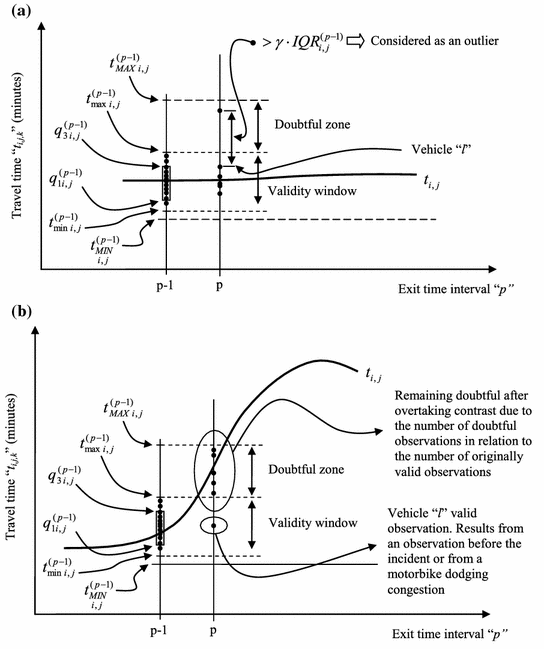

  

  Sketch of the overtaking contrast. a Elimination of an outlier. b Overtaking contrast does not make it possible to decide

• Congestion Contrast

  In case the overtaking contrast is not meaningful and “$t_{i,j,k}^{(p)}$” remains as a doubtful observation, the congestion contrast has the last word. As there does not exist a vehicle that has overtaken the vehicle “k” in a valid travel time, showing the evidence of the possibility of travelling within the validity window, the only possibility to decide if the observation results from a voluntary stop or from congestion in the itinerary is by estimating the traffic state within every highway section. If there is a high probability of congestion within some stretch of the itinerary, the observation is considered as valid. In contrast, if free flowing conditions are estimated, then the observation is considered an outlier.

Toll tickets are not the best data source to decide whether there is congestion or not in the highway in real time, due to the MTT nature of these data. Loop detector data would be more suitable for this objective (e.g. assessing the occupation at each loop detector), opening a gap for data fusion schemes. However, from toll tickets the origin destination matrix can be obtained on a reconstructed basis (i.e. once the vehicles have left the highway). Therefore, an approximation to the flow in each section can be obtained for the previous time interval (Daganzo 1997). Then, in the congestion contrast it is assumed that the probability of congestion in the present time interval depends on the traffic flow in the previous time interval. If this flow exceeds 75 % of the capacity of the infrastructure, a high probability of congestion is given to the highway section, and the observation is considered valid.

Highway capacities can be estimated using the HCM (Transportation Research Board 2000), but note that the capacity of an infrastructure is a dynamic variable and should be modified in case of an incident or bad weather conditions. Then, an accurate application of the data filtering process requires some kind of information input to modify default capacities in incident conditions. In addition, not only main trunk capacities must be assessed, also the exit toll gate capacities, as congestion can arise in the off-ramp due to limited exit capacity. These capacities can be easily obtained by taking into account the number of open gates and the type of these gates (i.e. manual payment—230 veh/h, automatic credit card payment—250 veh/h and non-stop ETC systems—700 veh/h).

5.1.3.2 5A.3.2 Deciding on Type 2 Doubtful Observations

An itinerary travel time observation falling in the lower doubtful zone can result from two situations:

• A motorbike dodging the traffic jam by wriggling between cars. This type of observation should be considered as an outlier.

• There is a sudden travel time decrease in the highway due to congestion dissipation. Then the observation should be considered as valid.

This type of outlier is not as problematic as the ones in excess, for two reasons. Firstly, there are few outliers of this nature. And secondly, in congestion dissipation, traffic flows at capacity, and it is not usual to find itineraries with few observations. On this basis, the doubtful observation is considered to be a motorbike if the difference between its travel time and the other existing valid observations in the set is considered large.

More formally, assuming there exists at least one valid observation in the set of observations where the doubtful “$t_{i,j,k}^{(p)}$” is contained, and vehicle “l” is the vehicle whose itinerary travel time, “$t_{i,j,l}^{(p)}$” is the minimum within the valid observations, then “$t_{i,j,k}^{(p)}$” is considered a motorbike if:

$$t_{i,j,k}^{(p)} \le t_{i,j,l}^{(p)} - \gamma \cdot IQR_{i,j}^{(p - 1)}$$

(5A.7)

In case Eq. (5A.7) holds, the observation is only considered as an outlier and eliminated if the number of originally valid observations in the set exceeds “${{N_{i,j}^{(p)} } \mathord{\left/ {\vphantom {{N_{i,j}^{(p)} } 2}} \right. \kern-0pt} 2}$”. Otherwise, the observation is considered as valid (see Fig. 5A.3).

Fig. 5A.3

Deciding on lower travel time doubtful observations. a Elimination of an outlier. b Validation of observations in a congestion dissipation situation

5.1.3.3 5A.3.3 Estimation of the Interquartile Range in Sets with Few Data

Once the data filtering process has decided on the validity of the observations in the set, and “$\hat{t}_{i,j}^{(p)}$” has been calculated as the median of the valid observations, the only remaining variable to estimate in order to set the confidence intervals for the next time interval (using Eqs. 5A.2 and 5A.4) is the interquartile range “$I\hat{Q}R_{i,j}^{(p)}$”. In the considered set with few data, the statistical calculations of “$\hat{q}_{{3\,i,j}}^{(p)}$” and “$\hat{q}_{{1 \, i,j}}^{(p)}$” are not meaningful. Therefore, it is assumed that the interquartile range does not vary from the last time interval. Under this assumption, the 25 % and the 75 % percentiles of the travel time distribution for the considered “p” time interval can be calculated as:

$$\begin{aligned} & \hat{q}_{{1{\kern 1pt} {\kern 1pt} {\kern 1pt} i,j}}^{(p)} = \hat{t}_{i,j}^{(p)} - (t_{i,j}^{(p - 1)} - q_{{1{\kern 1pt} {\kern 1pt} {\kern 1pt} i,j}}^{(p - 1)} ) \\ & \hat{q}_{{3{\kern 1pt} {\kern 1pt} {\kern 1pt} i,j}}^{(p)} = \hat{t}_{i,j}^{(p)} + (q_{{3{\kern 1pt} {\kern 1pt} {\kern 1pt} i,j}}^{(p - 1)} - t_{i,j}^{(p - 1)} ) \\ \end{aligned}$$

(5A.8)

5.1.4 5A.4 Sets with No Data

It can happen, particularly at nighttime, that there is no travel time observation for a particular itinerary (“$N_{i,j}^{(p)} = 0$”). Note that in this case “$\alpha_{i,j}^{(p)} = 0$”. The process to obtain “$t_{i,j}^{(p)}$” in this situation is simple. Travel times are assumed to maintain a linear constant evolution from the two last time intervals. This assumption is considered valid if at least one of these last time intervals has some observations. Otherwise, travel time is set to a default free flow travel time. The resulting formulation for sets with no data is:

$$t_{i,j}^{(p)} = \left\{ {\begin{array}{*{20}l} {t_{i,j}^{(p - 1)} + \left( {\frac{{\alpha_{i,j}^{(p - 1)} + \alpha_{i,j}^{(p - 2)} }}{2}} \right) \cdot \left( {t_{i,j}^{(p - 1)} - t_{i,j}^{(p - 2)} } \right)} & {if \; \alpha_{i,j}^{(p - 1)} > 0\quad or\quad \alpha_{i,j}^{(p - 2)} > 0} \\ {t_{i,j,0} } & {o.w.} \\ \end{array} } \right.$$

(5A.9)

In relation to the interquartile range, if “${\kern 1pt} \alpha_{i,j}^{(p - 1)} > 0{\kern 1pt}$” or “$\alpha_{i,j}^{(p - 2)} > 0{\kern 1pt} {\kern 1pt} {\kern 1pt}$” then it is calculated in the same way as in Sect. A.3.3. Otherwise the interquartile range is set to the default value “$IQR_{i,j,0}$”.

Taking into account the fact of the related values of “0” for the reliability indicator “$\alpha_{i,j}^{(p)}$” of the measurement, does not give any specific weight to these measurements in the smoothing equation for the next time intervals.

Appendix 5B: Accurate Formulation of the Basic Algorithm

Figure 5B.1 represents a zoom of the “i, i + 1” section of Fig. 5.2. From this figure it can be seen that Eq. (5.4) and by extension Eqs. (5.1), (5.3), (5.6), (5.7), (5.9), (5.11), (5.21), and (5.29) are not accurate.

Fig. 5B.1

Detailed sketch of a highway junction

To be accurate, Eq. (5.6) should be rewritten as:

$$t_{ex(i + 1)}^{{}} = t_{i,i + 1}^{{}} - t_{s - cut(i,i + 1)}^{{}} - t_{en(i)}^{{}}$$

(5B.1)

where the single section trimmed travel time can be obtained as:

$$t_{s - cut(i,i + 1)}^{{}} = \frac{{t_{s(i,i + 1)}^{{}} \cdot l_{s - cut(i,i + 1)}^{{}} }}{{l_{s(i,i + 1)}^{{}} }}$$

(5B.2)

with “$l_{s(i,i + 1)}^{{}}$” and “$l_{s - cut(i,i + 1)}^{{}}$” the section length and the trimmed section length respectively.

Applying the same modification to the two-section travel time, Eq. (5.11) should be rewritten as:

$$t_{ex2(i + 2)} = t_{i,i + 2} - t_{s - cut(i,i + 2)} - t_{en(i)}$$

(5B.3)

$$t_{s - cut(i,i + 2)}^{{}} = \frac{{t_{s(i,i + 2)}^{{}} \cdot \left( {l_{s(i,i + 1)}^{{}} + l_{s - cut(i + 1,i + 2)}^{{}} } \right)}}{{l_{s(i,i + 1)}^{{}} + l_{s(i + 1,i + 2)}^{{}} }}$$

(5B.4)

These modifications, which in practice have little consequence due to the magnitude of the section length in relation to the inner junction highway length, can also be applied to Eqs. (5.3), (5.9), (5.21) and (5.29).

This trimmed single section travel time can also be applied in the reconstruction of vehicle itineraries. Note that when reconstructing a trajectory by adding single section travel times, the last section travel time to consider must be a trimmed one.

Appendix 5C: Fusion of Different Estimations of Single Section Travel Times

From the basic and extended algorithm, different estimations of the single section travel times are obtained. Specifically, in an off-line application of the algorithm the following can be obtained:

• “$m - (i + 1)$” first order estimations of single section travel times “$t_{s(i,i + 1)}^{(p)}$”

• “$m - (i + 2)$” second order estimations of two section travel times “$t_{s(i,i + 2)}^{(p)}$”, which result in “$2 \cdot \left( {m - (i + 2)} \right)$” single section second order travel times “$t_{s2(i,i + 1)}^{(p)}$”.

In case of real time application, “m”, the ordinal number identifying the last exit in the highway should be replaced by its limitation “$i + n_{i}^{*(p)}$” (see Sect. 4.1).

5.1.1 5C.1 Fusion of First Order Single Section Travel Time Estimations

The objective of this data fusion is to obtain a representative average of the different estimations of a particular single section travel time. To do so, a simple weighted average is applied. The two aspects to consider in the determination of the weighting factor for each one of the estimations are:

• As the length of the itineraries used to estimate a single section travel time increase, the reliability of the estimation decreases. This accounts for the greater variance of the travel time distribution in longer itineraries, and for the decrease of the trajectories overlapping zone (see Sect. 4.1).

• An accuracy indicator of each single section travel time estimation can be obtained as the minimum of the statistical significances in the travel time itineraries that take part in the calculation, “$\min \left( {\alpha_{i,j}^{(p)} {\kern 1pt} {\kern 1pt} ,{\kern 1pt} {\kern 1pt} {\kern 1pt} {\kern 1pt} \alpha_{i + 1,j}^{(p)} } \right)$”.

Under these assumptions, the fused first order single section travel time is obtained as³:

$$t_{s1(i,i + 1)}^{(p)} = \frac{{\sum\nolimits_{j = i + 2}^{m} {\left\{ {\left[ {\frac{{1 + \min \left\{ {\alpha_{i,j}^{(q)} {\kern 1pt} {\kern 1pt} ,{\kern 1pt} {\kern 1pt} {\kern 1pt} {\kern 1pt} \alpha_{i + 1,j}^{(q)} } \right\}}}{{\ln \left( {j - i} \right)}}} \right] \cdot \left[ {(t_{i,j}^{(q)} - t_{en(i)} ) - (t_{i + 1,j}^{(q)} - t_{en(i + 1)} )} \right]} \right\}} }}{{\sum\nolimits_{j = 1 + 2}^{m} {\left[ {\frac{{1 + \min \left\{ {\alpha_{i,j}^{(q)} {\kern 1pt} {\kern 1pt} ,{\kern 1pt} {\kern 1pt} {\kern 1pt} {\kern 1pt} \alpha_{i + 1,j}^{(q)} } \right\}}}{{\ln \left( {j - i} \right)}}} \right]} }}$$

(5C.1)

Recall from Sect. 4.2 that “q” equals “p” for the real time application.

Again, the real time application version of Eq. (5C.1) is obtained by simply replacing “$i + n_{i}^{*(p)}$” instead of “m” and “p” instead of “q”.⁴

Taking into account the concepts detailed in Sect. 3.1 and Appendix 5B, the first order exit time is obtained as:

$$t_{ex1(i + 1)}^{(p)} = t_{i,i + 1}^{(p)} - t_{s1 - cut(i,i + 1)}^{(p)} - t_{en(i)}^{(p)}$$

(5C.2)

Finally, an accuracy indicator of these fused first order estimations is defined in Eq. (5C.3). These accuracy indicators only consider the first two estimations of the single section travel time, which are obtained from the shortest itineraries.

$$\begin{aligned} \alpha_{s1(i,i + 1)}^{(p)} &= \max \left\{ {\min \left\{ {\alpha_{(i,i + 2)}^{(q)} ,{\kern 1pt} {\kern 1pt} {\kern 1pt} {\kern 1pt} \alpha_{(i + 1,i + 2)}^{(q)} } \right\}{\kern 1pt} {\kern 1pt} ,{\kern 1pt} {\kern 1pt} {\kern 1pt} {\kern 1pt} \min \left\{ {\alpha_{(i,i + 3)}^{(q)} ,{\kern 1pt} {\kern 1pt} {\kern 1pt} {\kern 1pt} \alpha_{(i + 1,i + 3)}^{(q)} } \right\}} \right\} \hfill \\ \alpha_{ex1(i + 1)}^{(p)} &= \min \left\{ {\alpha_{(i,i + 1)}^{(p)} ,{\kern 1pt} {\kern 1pt} {\kern 1pt} {\kern 1pt} \alpha_{s1(i,i + 1)}^{(p)} } \right\} \hfill \\ \end{aligned}$$

(5C.3)

5.1.2 5C.2 Fusion of Second Order Single Section Travel Time Estimations

Proceeding in the same way and under the same assumptions of the previous section, the second order fused two-section travel time is obtained as:

$$t_{s2(i,i + 2)}^{(p)} = \frac{{\sum\nolimits_{j = i + 3}^{m} {\left\{ {\left[ {\frac{{1 + \min \left\{ {\alpha_{i,j}^{(q)} {\kern 1pt} {\kern 1pt} ,{\kern 1pt} {\kern 1pt} {\kern 1pt} {\kern 1pt} \alpha_{i + 2,j}^{(q)} } \right\}}}{{\ln \left( {j - i} \right)}}} \right] \cdot \left[ {(t_{i,j}^{(q)} - t_{en(i)} ) - (t_{i + 2,j}^{(q)} - t_{en(i + 2)} )} \right]} \right\}} }}{{\sum\nolimits_{j = i + 3}^{m} {\left[ {\frac{{1 + \min \left\{ {\alpha_{i,j}^{(q)} {\kern 1pt} {\kern 1pt} ,{\kern 1pt} {\kern 1pt} {\kern 1pt} {\kern 1pt} \alpha_{i + 2,j}^{(q)} } \right\}}}{{\ln \left( {j - i} \right)}}} \right]} }}$$

(5C.4)

To obtain the related fused second order single section travel time, recall Eqs. (5.13), (5.14), (5.15) and (5.16):

$$\begin{aligned} & \left. {\begin{array}{*{20}l} {t_{{s2(i,i + 1)}}^{{(p)}} = t_{{s2(i,i + 2)}}^{{(p)}} - t_{{s1(i + 1,i + 2)}}^{{(p)}} } \\ {t_{{s2(i + 1,i + 2)}}^{{(p)}} = t_{{s2(i,i + 2)}}^{{(p)}} - t_{{s2(i,i + 1)}}^{{(p)}} } \\ \end{array} } \right\}\quad if\;\alpha _{{s1(i + 1,i + 2)}}^{{(p)}} \ge \alpha _{{s1(i,i + 1)}}^{{(p)}} > 0 \\ & \left. {\begin{array}{*{20}l} {t_{{s2(i + 1,i + 2)}}^{{(p)}} = t_{{s2(i,i + 2)}}^{{(p)}} - t_{{s1(i,i + 1)}}^{{(p)}} } \\ {t_{{s2(i,i + 1)}}^{{(p)}} = t_{{s2(i,i + 2)}}^{{(p)}} - t_{{s2(i + 1,i + 2)}}^{{(p)}} } \\ \end{array} } \right\}\quad if\;\alpha _{{s1(i,i + 1)}}^{{(p)}} > \alpha _{{s1(i + 1,i + 2)}}^{{(p)}} > 0 \\ & \left. { \begin{array}{*{20}l} {t_{{s2(i,i + 1)}}^{{(p)}} = \frac{{t_{{s2(i,i + 2)}}^{{(p)}} \cdot l_{{s(i,i + 1)}} }}{{l_{{s(i,i + 2)}} }}} \\ {t_{{s2(i + 1,i + 2)}}^{{(p)}} = \frac{{t_{{s2(i,i + 2)}}^{{(p)}} \cdot l_{{s(i + 1,i + 2)}} }}{{l_{{s(i,i + 2)}} }}} \\ \end{array} } \right\}\quad if\;\alpha _{{s1(i,i + 1)}}^{{(p)}} = \alpha _{{s1(i + 1,i + 2)}}^{{(p)}} = 0 \\ \end{aligned}$$

(5C.5)

Finally, an accuracy indicator of these fused second order estimations of the single section travel times can also be defined as:

$$\begin{aligned} & \alpha_{s2(i,i + 1)}^{(p)} = \alpha_{s2(i + 1,i + 2)}^{(p)} = \min \left\{ {\alpha_{(i,i + 3)}^{(p)} ,{\kern 1pt} {\kern 1pt} {\kern 1pt} {\kern 1pt} \alpha_{(i + 2,i + 3)}^{(p)} ,{\kern 1pt} {\kern 1pt} {\kern 1pt} {\kern 1pt} \max \left\{ {\alpha_{s1(i,i + 1)}^{(p)} ,{\kern 1pt} {\kern 1pt} {\kern 1pt} {\kern 1pt} \alpha_{s1(i + 1,i + 2)}^{(p)} } \right\}} \right\} \\ & \alpha_{ex2(i + 2)}^{(p)} = \min \left\{ {\alpha_{(i,i + 2)}^{(p)} ,{\kern 1pt} {\kern 1pt} {\kern 1pt} {\kern 1pt} \alpha_{s2(i + 1,i + 2)}^{(p)} } \right\} \\ \end{aligned}$$

(5C.6)

5.1.3 5C.3 Fusion of First and Second Order Single Section Travel Times

To obtain the final estimation of the single section travel time “$t_{s(i,i + 1)}^{(p)}$”, it is only necessary to calculate a weighted average of first and second order estimations. The weighting factors are the accuracy indicators of each one of the estimations.

$$t_{s(i,i + 1)}^{(p)} = \frac{{\alpha_{s1(i,i + 1)}^{(p)} \cdot t_{s1(i,i + 1)}^{(p)} + \alpha_{{s2(i,i + 1)^{ + } }}^{(p)} \cdot t_{{s2(i,i + 1)^{ + } }}^{(p)} + \alpha_{{s2(i,i + 1)^{ - } }}^{(p)} \cdot t_{{s2(i,i + 1)^{ - } }}^{(p)} }}{{\alpha_{s1(i,i + 1)}^{(p)} + \alpha_{{s2(i,i + 1)^{ + } }}^{(p)} + \alpha_{{s2(i,i + 1)^{ - } }}^{(p)} }}$$

(5C.7)

Where the superscripts (+) and (−) in the second order estimations refer to the two possibilities of obtaining a single section travel time from a two-section travel time (i.e. “$t_{s2(i,i + 1)}^{(p)}$” can be obtained from “$t_{s1(i,i + 2)}^{(p)}$” and from “$t_{s1(i - 1,i + 1)}^{(p)}$”).

Applying a similar weighted average to the exit times:

$$t_{ex(i + 1)}^{(p)} = \frac{{\alpha_{ex1(i + 1)}^{(p)} \cdot t_{ex1(i + 1)}^{(p)} + \alpha_{ex2(i + 1)}^{(p)} \cdot t_{ex2(i + 1)}^{(p)} }}{{\alpha_{ex1(i + 1)}^{(p)} + \alpha_{ex2(i + 1)}^{(p)} }}$$

(5C.8)

Equations (5C.7) and (5C.8) are valid for “$i \in \left( {0,{\kern 1pt} \ldots ,{\kern 1pt} {\kern 1pt} m - 1} \right)$” (see Fig. 5.2). Note that for “i = 0” and for “i = m − 1”, some of the terms in Eqs. (5C.7) and (5C.8) are not defined (i.e. “$t_{{s2(i,i + 1)^{ + } }}^{(p)}$” is not defined for “i = m − 1”, “$t_{{s2(i,i + 1)^{ - } }}^{(p)}$” and “$t_{ex2(i + 1)}^{(p)}$” are not defined for “i = 0”). In these situations, the related accuracy indicators have a value of zero, and Eqs. (5C.7) and (5C.8) still hold.

References

Abdulhai, B., & Tabib, S. M. (2003). Spatio-temporal inductance-pattern recognition for vehicle reidentification. Transportation Research Part C, 11(3–4), 223–239.
Cassidy, M. J., & Ahn, S. (2005). Driver turn-taking behavior in congested freeway merges. Transportation Research Record, 1934, 140–147.
Coifman, B. (2001). Improved velocity estimation using single loop detectors. Transportation Research Part A, 35(10), 863–880.
Coifman, B. (2002). Estimating travel times and vehicle trajectories on freeways using dual loop detectors. Transportation Research Part A, 36(4), 351–364.
Coifman, B., & Cassidy, M. (2002). Vehicle reidentification and travel time measurement on congested freeways. Transportation Research Part A, 36(10), 899–917.
Coifman, B., & Ergueta, E. (2003). Improved vehicle reidentification and travel time measurement on congested freeways. ASCE Journal of Transportation Engineering, 129(5), 475–483.
Coifman, B., & Krishnamurthya, S. (2007). Vehicle reidentification and travel time measurement across freeway junctions using the existing detector infrastructure. Transportation Research Part C, 15(3), 135–153.
Cortés, C. E., Lavanya, R., Oh, J., & Jayakrishnan, R. (2002). General-purpose methodology for estimating link travel time with multiple-point detection of traffic. Transportation Research Record, 1802, 181–189.
Daganzo, C. F. (1997). Fundamentals of transportation and traffic operations. Pergamon: Elsevier.
Dailey, D. A. (1999). Statistical algorithm for estimating speed from single loop volume and occupancy measurements. Transportation Research Part B, 33(5), 313–322.
Davies, P., Hill, C., & Emmott, N. (1989). Automatic vehicle identification to support driver information systems. In Proceedings of IEEE Vehicle Navigation and Information Systems Conference, 11–13 September, A31–35.
Dion, F., & Rakha, H. (2006). Estimating dynamic roadway travel times using automatic vehicle identification data for low sampling rates. Transportation Research Part B, 40(9), 745–766.
Herrera, J. C., Work, D. B., Herring, R., Ban, X., Jacobson, Q., & Bayen, A. M. (2010). Evaluation of traffic data obtained via GPS-enabled mobile phones: the Mobile Century field experiment. Transportation Research Part C, 18(4), 568–583.
Hopkin, J., Crawford, D., & Catling, I. (2001). Travel time estimation. Summary of the European Workshop organized by the SERTI project, Avignon, November 2001.
Li, R., Rose, G., & Sarvi, M. (2007). Using automatic vehicle identification data to gain insight into travel time variability and its causes. Transportation Research Record 1945, 24–32.
Li, R., Rose, G., & Sarvi, M. (2006). Evaluation of speed-based travel time estimation models. ASCE Journal of Transportation Engineering, 132(7), 540–547.
Lucas, D. E., Mirchandani, P. B., & Verma, N. (2004). Online travel time estimation without vehicle identification. Transportation Research Record, 1867, 193–201.
Mikhalkin, B., Payne, H., & Isaksen, L. (1972). Estimation of speed from presence detectors. Highway Research Record, 388, 73–83.
Muñoz, J. C., & Daganzo, C. F. (2002). The bottleneck mechanism of a freeway diverge. Transportation Research Part A, 36(6), 483–505.
Nam, D. H., & Drew, D. R. (1996). Traffic dynamics: method for estimating freeway travel times in real time from flow measurements. ASCE Journal of Transportation Engineering, 122(3), 185–191.
Ohba, Y., Ueno, H., & Kuwahara, M. (1999). Travel time calculation method for expressway using toll collection system data. In Proceedings of the 2nd IEEE Intelligent Transportation Systems Conference, pp. 471–475.
Palen, J. (1997). The need for surveillance in intelligent transportation systems. Intellimotion, 6(1), 1–3.
Pushkar, A., Hall, F., & Acha-Daza, J. (1994). Estimation of speeds from single-loop freeway flow and occupancy data using cusp catastrophe theory model. Transportation Research Record, 1457, 149–157.
Sun, C., Ritchie, S. G., & Tsai, K. (1998). Algorithm development for derivation of section-related measures of traffic system performance using inductive loop detectors. Transportation Research Record, 1643, 171–180.
Sun, C., Ritchie, S. G., Tsai, K., & Jayakrishnan, R. (1999). Use of vehicle signature analysis and lexicographic optimization for vehicle reidentication on freeways. Transportation Research Part C, 7(4), 167–185.
SwRi, (1998). Automatic vehicle identification model deployment initiative—System design document. Report prepared for TransGuide, Texas Department of Transportation, Southwest Research Institute, San Antonio, TX.
Transportation Research Board. (2000). Highway capacity manual, Special Report 209, National Research Council, Washington, DC.
Turner, S. M., Eisele, W. L., Benz, R. J., & Holdener, D. J. (1998). Travel time data collection handBook. Research Report FHWA-PL-98-035. Federal Highway Administration, Office of Highway Information Management, Washington, DC.
van Arem, B., van der Vlist, M. J. M., Muste, M. R., & Smulders, S. A. (1997). Travel time estimation in the GERIDIEN project. International Journal of Forecasting, 13(1), 73–85.
van Lint, J. W. C., & van der Zijpp, N. J. (2003). Improving a travel-time estimation algorithm by using dual loop detectors. Transportation Research Record, 1855, 41–48.
Author information
Authors and Affiliations
Corresponding author