Generic Weakest Precondition Semantics from Monads Enriched with Order

Abstract

We devise a generic framework where a weakest precondition semantics, in the form of indexed posets, is derived from a monad whose Kleisli category is enriched by posets. It is inspired by Jacobs’ recent identification of a categorical structure that is common in various predicate transformers, but adds generality in the following aspects: (1) different notions of modality (such as “may” vs. “must”) are captured by Eilenberg-Moore algebras; (2) nested branching—like in games and in probabilistic systems with nondeterministic environments—is modularly modeled by a monad on the Eilenberg-Moore category of another.

These keywords were added by machine and not by the authors. This process is experimental and the keywords may be updated as the learning algorithm improves.

1 Introduction

Among various styles of program semantics, the one by predicate transformers [5] is arguably the most intuitive. Its presentation is inherently logical, representing a program’s behaviors by what properties (or predicates) hold before and after its execution. Predicate transformer semantics therefore form a basis of program verification, where specifications are given in the form of pre- and post-conditions [14]. It has also been used for refinement of specifications into programs (see e.g. [30]). Its success has driven extensions of the original nondeterministic framework, e.g. to the probabilistic one [18, 24] and to the setting with both nondeterministic and probabilistic branching [31].

A Categorical Picture. More recently, Jacobs in his series of papers [16, 17] has pushed forward a categorical view on predicate transformers. It starts with a monad $T$ that models a notion of branching. Then a program—henceforth called a (branching) computation—is a Kleisli arrow $X\rightarrow TY$; and the the weakest precondition semantics is given as a contravariant functor $\mathbb {P}^{\mathcal {K}{}\ell }:\mathcal {K}{}\ell (T)^{\mathop {\mathrm {op}}\nolimits }\rightarrow \mathbb {A}$, from the Kleisli category to the category $\mathbb {A}$ of suitable ordered algebras.

For example, in the basic nondeterministic setting, $T$ is the powerset monad $\mathcal P$ on $\mathbf {Sets}$ and $\mathbb {A}$ is the category $\mathbf {CL}_{\bigwedge }$ of complete lattices and $\bigwedge$-preserving maps. The weakest precondition functor $\mathbb {P}^{\mathcal {K}{}\ell }:\mathcal {K}{}\ell (T)^{\mathop {\mathrm {op}}\nolimits }\rightarrow \mathbf {CL}_{\bigwedge }$ then carries a function $f:X\rightarrow \mathcal PY$ to

$$\begin{aligned} \mathop {\mathrm {wpre}}(f){\;} : {\;}\mathcal PY\longrightarrow \mathcal PX\,, \qquad Q\longmapsto \{x\in X\mid f(x)\subseteq Q\} \,. \end{aligned}$$

(1)

Moreover it can be seen that: (1) the functor $\mathbb {P}^{\mathcal {K}{}\ell }$ factors through the comparison functor $K:\mathcal {K}{}\ell (\mathcal P)\rightarrow \mathcal {E}{}\mathcal {M}(\mathcal P)$ to the Eilenberg-Moore category $\mathcal {E}{}\mathcal {M}(\mathcal P)$; and (2) the extended functor $\mathbb {P}^{\mathcal {E}{}\mathcal {M}}$ has a dual adjoint $\mathbb {S}$. The situation is as follows.

(2)

Here the functor $K$ carries $f:X\rightarrow TY$ to $f^{\dagger }:\mathcal PX\rightarrow \mathcal PY, P\mapsto \bigcup _{x\in P}f(x)$ and is naturally thought of as a strongest postcondition semantics. Therefore the picture (2)—understood as the one below—identifies a categorical structure that underlies predicate transformer semantics. The adjunction here—it is in fact an isomorphism in the specific instance of (2)—indicates a “duality” between forward and backward predicate transformers.

(3)

Jacobs has identified other instances of (3) for: discrete probabilistic branching [16]; quantum logic [16]; and continuous probabilistic branching [17]. In all these instances the notion of effect module—originally from the study of quantum probability [6]—plays an essential role as algebras of “quantitative logics.”

Towards Generic Weakest Precondition Semantics. In [16, 17] the picture (3) is presented through examples and no categorical axiomatics—that induce the picture—have been explicitly introduced. Finding such is the current paper’s aim. In doing so, moreover, we acquire additional generality in two aspects: different modalities and nested branching.

To motivate the first aspect, observe that the weakest precondition semantics in (1) is the must semantics. The may variant looks as interesting; it would carry a postcondition $Q\subseteq Y$ to $\{x\in X\mid f(x)\cap Q\ne \emptyset \}$. The difference between the two semantics is much like the one between the modal operators $\Box$ and $\Diamond$.

On the second aspect, situations are abound in computer science where a computation involves two layers of branching. Typically these layers correspond to two distinct players with conflicting interests. Examples are games, a two-player version of automata which are essential tools in various topics including model-checking; and probabilistic systems where it is common to include nondeterministic branching too for modeling the environment’s choices. Further details will be discussed later in Sect. 3.

Predicates and Modalities from Monads. In this paper we present two categorical setups that are inspired by [4, 23]—specifically by their use of $T1$ as a domain of truth values or quantities.

The first “one-player” setup is when we have only one layer of branching. Much like in [16, 17] we start from a monad $T$. Assuming that $T$ is order-enriched—in the sense that its Kleisli category $\mathcal {K}{}\ell (T)$ is $\mathbf {Posets}$-enriched—we observe that:

• a natural notion of truth value arises from an object $T\varOmega$ (typically $\varOmega =1$);

• and a modality (like “may” and “must”) corresponds to a choice of an Eilenberg-Moore algebra $\tau :T(T\varOmega )\rightarrow T\varOmega$.

The required data set $(T,\varOmega ,\tau )$ shall be called a predicate transformer situation. We prove that it induces a weakest precondition semantics functor $\mathcal {K}{}\ell (T)^{\mathop {\mathrm {op}}\nolimits }\rightarrow \mathbf {Posets}$, and that it factors through $K:\mathcal {K}{}\ell (T)\rightarrow \mathcal {E}{}\mathcal {M}(T)$, much like in (2). The general setup addresses common instances like the original nondeterministic one [5] and the probabilistic predicate transformers in [18, 24]. Moreover it allows us to systematically search for different modalities, leading e.g. to a probabilistic notion of partial correctness guarantee (which does not seem well-known).

The other setup is the “two-player” one. It is much like a one-player setup built on another, with two monads $T$ and $R$ and two “modalities” $\tau$ and $\rho$. A potential novelty here is that $R$ is a monad on $\mathcal {E}{}\mathcal {M}(T)$; this way we manage some known complications in nested branching, such as the difficulty of combining probability and nondeterminism. We prove that the data set $(T,\varOmega ,\tau ,R,\rho )$ gives rise to a weakest precondition semantics, as before. Its examples include: a logic of forced predicates in games; and the probabilistic predicate transformers in [31].

In this paper we focus on one side of predicate transformers, namely weakest precondition semantics. Many components in the picture of [16, 17] are therefore left out. They include the adjoint $\mathbb {S}$ in (3), and the role of effect modules. Indeed, on the top-left corner of (3) we always have $\mathbf {Posets}$ which is less rich a structure than complete lattices or effect modules. Incorporating these is future work.

Organization of the Paper. In Sect. 2 we introduce our first “one-player” setup, and exhibit its examples. Our second “two-player” setup is first motivated in Sect. 3 through the examples of games and probabilistic systems, and is formally introduced in Sect. 4. Its examples are described in Sect. 5 in detail. In Sect. 6 we conclude.

(4)

Notations and Terminologies. For a monad $T$, a $T$ -algebra $TX\mathop {\rightarrow }\limits ^{a}X$ shall always mean an Eilenberg-Moore algebra for $T$, making the diagrams on the right commute. For categorical backgrounds see e.g. [1, 28].

Given a monad $T$ on $\mathbb {C}$, an arrow in the Kleisli category $\mathcal {K}{}\ell (T)$ is denoted by ; an identity arrow is by $\mathrm {id}^{\mathcal {K}{}\ell (T)}_{X}$; and composition of arrows is by $g\mathbin {\odot }f$. These are to be distinguished from $X\rightarrow Y$, $\mathrm {id}_{X}$ and $g\mathrel {\circ }f$ in the base category $\mathbb {C}$.

2 Generic Weakest Preconditions, One-Player Setting

2.1 Order-Enriched Monad

We use monads for representing various notions of “branching.” These monads are assumed to have order-enrichment ($\sqsubseteq$ for, roughly speaking, “more options”); and this will be used for an entailment relation, an important element of logic.

The category $\mathbf {Posets}$ is that of posets and monotone functions.

Definition 2.1

An order-enriched monad $T$ on a category $\mathbb {C}$ is a monad together with a $\mathbf {Posets}$-enriched structure of the Kleisli category $\mathcal {K}{}\ell (T)$.

The latter means specifically: (1) each homset $\mathcal {K}{}\ell (T)(X,Y)=\mathbb {C}(X,TY)$ carries a prescribed poset structure; and (2) composition $\mathbin {\odot }$ in $\mathcal {K}{}\ell (T)$ is monotone in each argument. Such order-enrichment typically arises from the poset structure of $TY$ in the pointwise manner. In the specific setting of $\mathbb {C}=\mathbf {Sets}$ such enrichment can be characterized by substitutivity and congruence of orders on $TX$; see [21].

Below are some examples of order-enriched monads. Our intuition about an order-enriched monad $T$ is that it represents one possible branching type, where $\eta _{X}:X\rightarrow TX$ represents the trivial branching with a unique option and $\mu _{X}:T(TX)\rightarrow TX$ represents flattening ‘branching twice’ into ‘branching once’ (see [13]). In fact each of the examples below has the Kleisli category $\mathcal {K}{}\ell (T)$ enriched by the category $\mathbf {Cppo}$ of pointed cpo’s and continuous maps—not just by $\mathbf {Posets}$—and hence is suited for generic coalgebraic trace semantics [13].

Example 2.2

 

• 1. The lift monad $\mathcal {L}=1+(\underline{}\,)$—where the element of $1$ is denoted by $\bot$—has a standard monad structure induced by coproducts. For example, the multiplication $\mu ^{\mathcal {L}}:1+1+X\rightarrow 1+X$ carries $x\in X$ to itself and both $\bot$’s to $\bot$. The set $\mathcal {L}X$ is a pointed dcpo with the flat order ($\bot \sqsubseteq x$ for each $x\in X$).

  The lift monad $\mathcal {L}$ models the “branching type” of potential nontermination.

• 2. The powerset monad $\mathcal P$ models (possibilistic) nondeterminism. Its action on arrows takes direct images: $(\mathcal Pf)U=\{f(x)\mid x\in U\}$. Its unit is given by singletons: $\eta ^{\mathcal P}_{X}=\{\underline{}\,\}:X\rightarrow \mathcal PX$, and its multiplication is by unions: $\mu ^{\mathcal P}_{X}=\bigcup :\mathcal P(\mathcal PX) \rightarrow \mathcal PX$.

• 3. The subdistribution monad $\mathcal D\!$ models probabilistic branching. It carries a set $X$ to the set of (probability) subdistributions over $X$:

  $$\begin{aligned} \mathcal D\!X \;:=\; \textstyle \bigl \{d:X\rightarrow [0,1]\;\bigl |\bigr .\;\sum _{x\in X}d(x)\le 1\bigr \}\,; \end{aligned}$$

  such $d$ is called a subdistribution since the values need not add to $1$. Given an arrow $f:X\rightarrow Y$ in $\mathbf {Sets}$, $\mathcal D\!f:\mathcal D\!X\rightarrow \mathcal D\!Y$ is defined by $(\mathcal D\!f)(d)(y):= \sum _{x\in f^{-1}(\{y\})}d(x)$. Its unit is the Dirac (or pointmass) distribution: $\eta ^{\mathcal D\!}_{X}(x) = [\,x\mapsto 1;\, x'\mapsto 0\;(\mathrm{for}~x'\ne x)]$; its multiplication is defined by $\mu ^{\mathcal D\!}_{X}(\mathfrak {a}) \;=\; [x\mapsto \sum _{d\in \mathcal D\!X}\mathfrak {a}(d)\cdot d(x)]$ for $\mathfrak {a}\in \mathcal D\!(\mathcal D\!X)$.

Besides, the quantum branching monad $\mathcal {Q}$ is introduced in [12] for the purpose of modeling a quantum programming language that obeys the design principle of “quantum data, classical control.” It comes with an order-enrichment, too, derived from the Löwner partial order between positive operators. Yet another example is the continuous variant of $\mathcal D\!$, namely the Giry monad on the category $\mathbf {Meas}$ of measurable spaces [7].

2.2 PT Situation and Generic Weakest Precondition Semantics

We introduce our first basic setup for our generic weakest precondition semantics. In our main examples we take $\mathbb {C}=\mathbf {Sets}$ and $\varOmega =1$ (a singleton).

Definition 2.2

(PT situation). A predicate transformer situation (a PT situation for short) over a category $\mathbb {C}$ is a triple $(T, \varOmega , \tau )$ of

• an order-enriched monad $T$ on $\mathbb {C}$;

• an object $\varOmega \in \mathbb {C}$; and

• an (Eilenberg-Moore) algebra $\tau :T(T\varOmega )\rightarrow T\varOmega$ that satisfies the following monotonicity condition: for each $X\in \mathbb {C}$, the correspondence

  $$\begin{aligned} (\varPhi _{\tau })_{X} \;:\;&\mathbb {C}(X, T\varOmega ) \longrightarrow \mathbb {C}(TX, T\varOmega ) \,, \; \text {i.e.}\; \mathcal {K}{}\ell (T)(X, \varOmega ) \longrightarrow \mathcal {K}{}\ell (T)(TX, \varOmega ) \,, \\&\text {given by}\quad \bigl (X\mathop {\rightarrow }\limits ^{p}T\varOmega \bigr ) \longmapsto \bigl (TX\mathop {\rightarrow }\limits ^{Tp}T(T\varOmega )\mathop {\rightarrow }\limits ^{\tau }T\varOmega \bigr )\,\end{aligned}$$

  is monotone with respect to the order-enrichment of the Kleisli category $\mathcal {K}{}\ell (T)$ (Definition 2.1). Note here that $\varPhi _{\tau }:\mathbb {C}(\underline{}\,,T\varOmega )\Rightarrow \mathbb {C}(T\underline{}\,,T\varOmega )$ is nothing but the natural transformation induced by the arrow $\tau$ via the Yoneda lemma.

The data $\tau$ is called a modality; see the introduction (Sect. 1) and also Sect. 2.3 below.

The following lemma gives a canonical (but not unique) modality for $T$.

Lemma 2.4

If $T$ is an order-enriched monad, $(T,\varOmega ,\mu _{\varOmega })$ is a PT situation.

Proof

We have only to check the monotonicity condition of $\mu _{\varOmega }$ in Definition 2.2. It is easy to see that $(\varPhi _{\mu _{\varOmega }})_{X}=\mu _{\varOmega }\mathrel {\circ }T(\underline{}\,):\mathbb {C}(X,T\varOmega )\rightarrow \mathbb {C}(TX,T\varOmega )$ is equal to $(\underline{}\,)\mathbin {\odot }(\mathrm {id}_{TX})^{\wedge }:\mathcal {K}{}\ell (T)(X,\varOmega )\rightarrow \mathcal {K}{}\ell (T)(TX,\varOmega )$. Here is the arrow that corresponds to the identity $\mathrm {id}_{TX}$ in $\mathbb {C}$. The claim follows from the monotonicity of $\mathbin {\odot }$.    $\square$

We shall derive a weakest precondition semantics from a given PT situation $(T,\varOmega ,\tau )$. The goal would consist of:

• a (po)set $\mathbb {P}^{\mathcal {K}{}\ell }(\tau )(X)$ of predicates for each object $X\in \mathbb {C}$, whose order $\sqsubseteq$ represents an entailment relation between predicates; and

• an assignment, to each (branching) computation $f:X\rightarrow TY$ in $\mathbb {C}$, a predicate transformer

  $$\begin{aligned} \mathop {\mathrm {wpre}}(f) \;:\; \mathbb {P}^{\mathcal {K}{}\ell }(\tau )(Y) \longrightarrow \mathbb {P}^{\mathcal {K}{}\ell }(\tau )(X) \end{aligned}$$

  (5)

  that is a monotone function.

Since a computation is an arrow in $\mathcal {K}{}\ell (T)$, we are aiming at a functor

$$\begin{aligned} \mathbb {P}^{\mathcal {K}{}\ell }(\tau ) \;:\; \mathcal {K}{}\ell (T)^{\mathop {\mathrm {op}}\nolimits } \longrightarrow \mathbf {Posets}\,. \end{aligned}$$

(6)

Such a functor is known as an indexed poset, a special case of indexed categories. These “indexed” structures are known to correspond to “fibered” structures (poset fibrations and (split) fibrations, respectively), and all these have been used as basic constructs in categorical logic (see e.g. [15]). An indexed poset like (6) therefore puts us on a firm footing.

Proposition 2.5

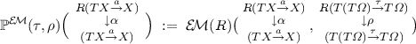
(the indexed poset $\mathbb {P}^{\mathcal {K}{}\ell }(\tau )$ ). Given a PT situation $(T,\varOmega ,\tau )$, the following defines an indexed poset $\mathbb {P}^{\mathcal {K}{}\ell }(\tau ):\mathcal {K}{}\ell (T)^{\mathop {\mathrm {op}}\nolimits } \rightarrow \mathbf {Posets}$.¹

• On an object $X\in \mathcal {K}{}\ell (T)$, $\mathbb {P}^{\mathcal {K}{}\ell }(\tau )(X):=\mathcal {K}{}\ell (T)(X,\varOmega )=\mathbb {C}(X,T\varOmega )$.

• On an arrow , $\mathbb {P}^{\mathcal {K}{}\ell }(\tau )(f) :\mathbb {C}(Y,T\varOmega ) \rightarrow \mathbb {C}(X,T\varOmega )$ is defined by

  $$\begin{aligned} \bigl (\, Y\mathop {\rightarrow }\limits ^{q}T\varOmega \,\bigr ) \;\longmapsto \; \bigl (\, X\mathop {\rightarrow }\limits ^{f} TY\mathop {\rightarrow }\limits ^{Tq} T(T\varOmega ) \mathop {\rightarrow }\limits ^{\tau } T\varOmega \,\bigr )\,. \end{aligned}$$

Proof

We need to check: the monotonicity of $\mathbb {P}^{\mathcal {K}{}\ell }(\tau )(f)$; and that the functor $\mathbb {P}^{\mathcal {K}{}\ell }(\tau )$ indeed preserves identities and composition of arrows. These will be proved later, altogether in the proof of Theorem 2.10.    $\square$

A consequence of the proposition—specifically the functoriality of $\mathbb {P}^{\mathcal {K}{}\ell }(\tau )$—is compositionality of the weakest precondition semantics: given two computations $f:X\rightarrow TY$, $g:Y\rightarrow TU$ and a postcondition $r:U\rightarrow T1$, we have

$$\begin{aligned} \mathbb {P}^{\mathcal {K}{}\ell }(\tau )(g\mathbin {\odot }f)(r) \;=\; \mathbb {P}^{\mathcal {K}{}\ell }(\tau )(f)\bigl (\, \mathbb {P}^{\mathcal {K}{}\ell }(\tau )(g)(r) \,\bigr )\,. \end{aligned}$$

That is, the semantics of a sequential composition $g\mathbin {\odot }f$ can be computed step by step.

2.3 Examples of PT Situations

For each of $T=\mathcal {L}, \mathcal P, \mathcal D\!$ in Example 2.2, we take $\varOmega =1$ and the set $T1$ is naturally understood as a set of “truth values” (an observation in [4, 23]):

Here $*$ is the element of the argument $1$ in $\mathcal {L}1$. Both $\mathcal {L}1$ and $\mathcal P1$ represent the Boolean truth values. In the $\mathcal D\!$ case a truth value is $r\in [0,1]$; a predicate, being a function $X\rightarrow [0,1]$, is hence a random variable that tells the certainty with which the predicate holds at each $x\in X$.

We shall introduce modalities for these monads $T$ and $\varOmega =1$. The following observation (easy by diagram chasing) will be used.

Lemma 2.6

The category $\mathcal {E}{}\mathcal {M}(T)$ of Eilenberg-Moore algebra is iso-closed in the category of functor $T$-algebras. That is, given an Eilenberg-Moore algebra $a:TX\rightarrow X$, an arrow $b:TY\rightarrow Y$, and an isomorphism such that $f\mathrel {\circ }a=b\mathrel {\circ }Tf$, the arrow $b$ is also an Eilenberg-Moore algebra.    $\square$

The Lift Monad ${\varvec{\mathcal {L}: \tau _{\mathrm {total}}}}$ and ${\varvec{\tau _{\mathrm {partial}}.}}$ We have the following two modalities (and none other, as is easily seen).

$$\begin{aligned} \begin{array}{rl} \tau _{\mathrm {total}}, \tau _{\mathrm {partial}}\;:&{} \{\bot \}+\{\mathtt {t{}t}, \mathtt {f{}f}\}=\mathcal {L}(\mathcal {L}1) \quad \longrightarrow \quad \mathcal {L}1= \{\mathtt {t{}t}, \mathtt {f{}f}\}\,, \\ \tau _{\mathrm {total}}\;:&{} \bot \mapsto \mathtt {f{}f}\,,\quad \mathtt {t{}t}\mapsto \mathtt {t{}t}\,,\quad \mathtt {f{}f}\mapsto \mathtt {f{}f}\,, \\ \tau _{\mathrm {partial}}\;:&{} \bot \mapsto \mathtt {t{}t}\,,\quad \mathtt {t{}t}\mapsto \mathtt {t{}t}\,,\quad \mathtt {f{}f}\mapsto \mathtt {f{}f}\,. \end{array} \end{aligned}$$

The one we obtain from multiplication $\mu ^{\mathcal {L}}_{1}$ is $\tau _{\mathrm {total}}$; the other $\tau _{\mathrm {partial}}$ is nonetheless important in program verification. Given $q:Y\rightarrow \mathcal {L}1$ and $f:X\rightarrow \mathcal {L}Y$ where $f$ is understood as a possibly diverging computation from $X$ to $Y$, the predicate

$$\begin{aligned} \mathbb {P}^{\mathcal {K}{}\ell }(\tau _{\mathrm {partial}}) (f)(q) = \tau _{\mathrm {partial}}\mathrel {\circ }\mathcal {L}q\mathrel {\circ }f \quad :\quad X\longrightarrow \mathcal {L}1 \end{aligned}$$

carries $x\in X$ to $\mathtt {t{}t}$ in case $f(x)=\bot$, i.e., if the computation is diverging. This is therefore a partial correctness specification that is common in Floyd-Hoare logic (see e.g. [37]). In contrast, using $\tau _{\mathrm {total}}$, the logic is about total correctness.

The Powerset Monad ${\varvec{\mathcal P}}$: ${\varvec{\tau _{\Diamond }}}$ and ${\varvec{\tau _{\Box }.}}$ The monad multiplication $\mu ^{\mathcal P}_{1}$ yields a modality which shall be denoted by $\tau _{\Diamond }$. The other modality $\tau _{\Box }$ is given via the swapping :

(7)

In view of Lemma 2.6, we have only to check that the map $\tau _{\Box }$ satisfies the monotonicity condition in Definition 2.2. We first observe that, for $h:X\rightarrow \mathcal P1$ and $U\in \mathcal PX$,

$$\begin{aligned} (\tau _{\Box }\mathrel {\circ }\mathcal Ph)(U)=\mathtt {f{}f}\quad \Longleftrightarrow \quad \mathtt {f{}f}\in (\mathcal Ph)(U) \quad \Longleftrightarrow \quad \exists x\in U.\, h(x)=\mathtt {f{}f}\,, \end{aligned}$$

where the first equivalence is by (7). Now assume that and $(\tau _{\Box }\mathrel {\circ }\mathcal Pg)(U)=\mathtt {f{}f}$. For showing $\tau _{\Box }\mathrel {\circ }\mathcal Pf\sqsubseteq \tau _{\Box }\mathrel {\circ }\mathcal Pg$ it suffices to show that $(\tau _{\Box }\mathrel {\circ }\mathcal Pf)(U)=\mathtt {f{}f}$; this follows from the above observation.

The modalities $\tau _{\Diamond }$ and $\tau _{\Box }$ capture the may and must weakest preconditions, respectively. Indeed, given a postcondition $q:Y\rightarrow \mathcal P1$ and $f:X\rightarrow \mathcal PY$, we have $\mathbb {P}^{\mathcal {K}{}\ell }(\tau _{\Diamond })(f)(q)(x)=\mathtt {t{}t}$ if and only if there exists $y\in Y$ such that $y\in f(x)$ and $q(y)=\mathtt {t{}t}$; and $\mathbb {P}^{\mathcal {K}{}\ell }(\tau _{\Box }) (f)(q)(x)=\mathtt {t{}t}$ if and only if $y\in f(x)$ implies $q(y)=\mathtt {t{}t}$.

Moreover, we can show that $\tau _{\Diamond }$ and $\tau _{\Box }$ are the only modalities (in the sense of Definition 2.2) for $T=\mathcal P$ and $\varOmega =1$. Since the unit law in (4) forces $\tau \{\mathtt {t{}t}\}=\mathtt {t{}t}$ and $\tau \{\mathtt {f{}f}\}=\mathtt {f{}f}$, the only possible variations are the following $\tau _{1}$ and $\tau _{2}$ (cf. (7)):

$$\begin{aligned} \tau _{1}\{\}=\mathtt {t{}t}\,,\; \tau _{1}\{\mathtt {t{}t},\mathtt {f{}f}\}=\mathtt {t{}t}\,; \quad \tau _{2}\{\}=\mathtt {f{}f}\,,\; \tau _{2}\{\mathtt {t{}t},\mathtt {f{}f}\}=\mathtt {f{}f}\,. \end{aligned}$$

Both of these, however, fail to satisfy the multiplication law in (4).

The monotonicity condition in Definition 2.2, in the case of $T\in \{\mathcal {L},\mathcal P\}$ (hence $T\varOmega \cong 2$), coincides with monotonicity of a predicate lifting $2^{(\underline{}\,)}\Rightarrow 2^{T(\underline{}\,)}$. The latter is a condition commonly adopted in coalgebraic modal logic (see e.g. [25]).

The Subdistribution Monad ${\varvec{\mathcal D\!:}}$ ${\varvec{\tau _{\mathrm {total}}}}$ and ${\varvec{\tau _{\mathrm {partial}}.}}$    The modality $\tau _{\mathrm {total}}: \mathcal D\![0,1]\rightarrow [0,1]$ that arises from the multiplication $\mu ^{\mathcal D\!}_{1}$ is such that: given $q:Y\rightarrow \mathcal D\!1$ and $f:X\rightarrow \mathcal D\!Y$, we have $\mathbb {P}^{\mathcal {K}{}\ell }(\tau _{\mathrm {total}}) (f)(q)(x)=\sum _{y\in Y} q(y) \cdot f(x)(y)$. This is precisely the expected value of the random variable $q$ under the distribution $f(x)$; thus $\tau _{\mathrm {total}}$ yields the probabilistic predicate transformer of [18, 24].

In parallel to the powerset monad case, we have an isomorphism . Another modality $\tau _{\mathrm {partial}}:\mathcal D\![0,1]\rightarrow [0,1]$ then arises by $\tau _{\mathrm {partial}}:=\sigma \mathrel {\circ }\tau _{\mathrm {total}}\mathrel {\circ }\mathcal D\!\sigma$ like in (7), for which we have

$$\begin{aligned} \tau _{\mathrm {partial}}(d)\;&=\;\textstyle \bigl (1-\sum _{r\in [0,1]}d(r)\bigr )+\sum _{r\in [0,1]}r\cdot d(r) \quad \text {and} \\ \mathbb {P}^{\mathcal {K}{}\ell }(\tau _{\mathrm {partial}}) (f)(q)(x) \;&=\;\textstyle \bigl (1-\sum _{y\in Y}f(x)(y)\bigr )+\sum _{y\in Y} q(y) \cdot f(x)(y)\,. \end{aligned}$$

In the second line, the value $1-\sum _{y\in Y}f(x)(y)$—the probability of $f$’s divergence—is added to the $\tau _{\mathrm {total}}$ case. Therefore the modalities $\tau _{\mathrm {partial}}$ and $\tau _{\mathrm {total}}$, much like in the case of $T=\mathcal {L}$, carry the flavor of partial and total correctness guarantee.

To see that $\tau _{\mathrm {partial}}$ is indeed a modality is easy: we use Lemma 2.6; and the monotonicity can be deduced from the following explicit presentation of $\tau _{\mathrm {partial}}\mathrel {\circ }\mathcal D\!p$ for $p:X\rightarrow \mathcal D\!1=[0,1]$. For each $d\in \mathcal D\!X$,

$$\begin{aligned} \textstyle (\tau _{\mathrm {partial}}\mathrel {\circ }\mathcal D\!p)(d) \;&= \; \textstyle \tau _{\mathrm {partial}}\Bigl [ r\mapsto \sum _{x\in p^{-1}(\{r\})} d(x) \Bigr ]_{r\in [0,1]} \\ \;&= \;\textstyle \bigl ( 1-\sum _{r\in [0,1]} \sum _{x\in p^{-1}(\{r\})} d(x) \bigr ) + \sum _{r\in [0,1]}r\sum _{x\in p^{-1}(\{r\})} d(x) \\ \;&= \;\textstyle \bigl ( 1-\sum _{x\in X} d(x) \bigr ) + \sum _{x\in X} p(x)\cdot d(x)\,. \end{aligned}$$

We do not yet know if $\tau _{\mathrm {total}}$ and $\tau _{\mathrm {partial}}$ are the only modalities for $\mathcal D\!$ and $\varOmega =1$.

Remark 2.7

We note the difference between a subdistribution $d\in \mathcal D\!X$ and a predicate (i.e. a random variable) $p:X\rightarrow \mathcal D\!1$. An example of the latter is $p_{\top }$ that is everywhere $1$—this is the truth predicate. In contrast, the former $d\in \mathcal D\!X$ is subject to the (sub)normalization condition $\sum _{x}d(x)\le 1$. We understand it as one single “current state” whose whereabouts are known only probabilistically.

2.4 Factorization via the Eilenberg-Moore Category

The indexed poset $\mathbb {P}^{\mathcal {K}{}\ell }(\tau ):\mathcal {K}{}\ell (T)^{\mathop {\mathrm {op}}\nolimits }\rightarrow \mathbf {Posets}$ in Proposition 2.5 is shown here to factor through the comparison functor $K:\mathcal {K}{}\ell (T)\rightarrow \mathcal {E}{}\mathcal {M}(T)$, much like in (2). In fact it is possible to see $K$ as a strongest postcondition semantics; see Remark 2.11.

We will be using the following result.

Lemma 2.8

Let $T$ be an order-enriched monad on $\mathbb {C}$, $X,Y,U\in \mathbb {C}$ and $f:X\rightarrow Y$ be an arrow in $\mathbb {C}$. Then $(\underline{}\,)\mathrel {\circ }f:\mathbb {C}(Y,TU)\rightarrow \mathbb {C}(X, TU)$ is monotone.

Proof

Given $g:Y\rightarrow TU$ in $\mathbb {C}$,

where $J:\mathbf {Sets}\rightarrow \mathcal {K}{}\ell (T)$ is the Kleisli inclusion that sends the arrow $\eta _{X}:X\rightarrow TX$ to . In the calculation we used the monad laws as well as the naturality of $\eta$ and $\mu$. The correspondence $(\underline{}\,)\mathbin {\odot }(Tf\mathbin {\odot }J\eta _{X})$ is monotone by assumption (Definition 2.1); this proves the claim.    $\square$

Proposition 2.9

(the indexed poset $\mathbb {P}^{\mathcal {E}{}\mathcal {M}}(\tau )$ ). A PT situation $(T,\varOmega ,\tau )$ induces an indexed poset $\mathbb {P}^{\mathcal {E}{}\mathcal {M}}(\tau ):\mathcal {E}{}\mathcal {M}(T)^{\mathop {\mathrm {op}}\nolimits } \rightarrow \mathbf {Posets}$ in the following way.

• On objects,

  

  where the order $\sqsubseteq$ on the set $\mathcal {E}{}\mathcal {M}(T)(a,\tau )$ is inherited from $\mathbb {C}(X,T\varOmega )$ via the forgetful functor $U^{T}:\mathcal {E}{}\mathcal {M}(T)\rightarrow \mathbb {C}$.

• On an arrow $f:(TX\mathop {\rightarrow }\limits ^{a}X)\rightarrow (TY\mathop {\rightarrow }\limits ^{b}Y)$,

  

Proof

The monotonicity of $\mathbb {P}^{\mathcal {E}{}\mathcal {M}}(\tau )(f)$ follows from the order-enrichment of $T$ via Lemma 2.8. The functoriality of $\mathbb {P}^{\mathcal {E}{}\mathcal {M}}(\tau )$ is obvious.    $\square$

Theorem 2.10

For a PT situation $(T,\varOmega ,\tau )$, the following diagram commutes up-to a natural isomorphism. Here $K$ is the comparison functor.

(8)

Proof

(Also of Proposition 2.5) The natural isomorphism $\varPsi$ in question is of the type

and it is defined by the adjunction $\mathbb {C}(X,U^{T}\tau )\cong \mathcal {E}{}\mathcal {M}(T)(\mu _{X},\tau )$ where $U^{T}$ is the forgetful functor. Explicitly: $\varPsi _{X}\bigl (X\mathop {\rightarrow }\limits ^{p}T\varOmega \bigr )=\bigl (TX\mathop {\rightarrow }\limits ^{Tp} T(T\varOmega )\mathop {\rightarrow }\limits ^{\tau } T\varOmega \bigr )$; and its inverse is $\varPsi _{X}^{-1}\bigl (TX\mathop {\rightarrow }\limits ^{f} T\varOmega \bigr )=\bigl (X\mathop {\rightarrow }\limits ^{\eta _{X}}TX\mathop {\rightarrow }\limits ^{f}T\varOmega \bigr )$. The function $\varPsi _{X}$ is monotonic by the monotonicity of $\tau$, see Definition 2.2; so is its inverse $\varPsi _{X}^{-1}$ by Lemma 2.8.

Let us turn to naturality of $\varPsi$. Given in $\mathcal {K}{}\ell (T)$, it requires

(9)

Indeed, given $q:Y\rightarrow T\varOmega$,

$$\begin{aligned}&\mathbb {P}^{\mathcal {E}{}\mathcal {M}}(\tau )(Kf)(\varPsi _{Y} q) = \mathbb {P}^{\mathcal {E}{}\mathcal {M}}(\tau )(Kf)(\tau \mathrel {\circ }Tq) = \tau \mathrel {\circ }Tq\mathrel {\circ }\mu _{Y}\mathrel {\circ }Tf \\&\ \ \ \ = \tau \mathrel {\circ }\mu _{T\varOmega }\mathrel {\circ }T(Tq)\mathrel {\circ }Tf = \tau \mathrel {\circ }T\tau \mathrel {\circ }T(Tq)\mathrel {\circ }Tf = \bigl (\varPsi _{X}\mathrel {\circ }\mathbb {P}^{\mathcal {K}{}\ell }(\tau )(f)\bigr )q\,, \end{aligned}$$

where the third equality is naturality of $\mu$ and the fourth is the multiplication law of $\tau$ (see (4)). By this naturality, in particular, we have that $\mathbb {P}^{\mathcal {K}{}\ell }(\tau )(f)$ is monotone (since the other three arrows are monotone). This is one property needed in Proposition 2.5; the other—functoriality of $\mathbb {P}^{\mathcal {K}{}\ell }(\tau )$—also follows from naturality of $\varPsi$, via the functoriality of $K$ and $\mathbb {P}^{\mathcal {E}{}\mathcal {M}}(\tau )$.    $\square$

Remark 2.11

The comparison functor $K:\mathcal {K}{}\ell (T)\rightarrow \mathcal {E}{}\mathcal {M}(T)$ can be seen as a strongest postcondition semantics. Given a (branching) computation $f:X\rightarrow TY$, we obtain

$$\begin{aligned} \mathop {\mathrm {spost}}\nolimits (f) := \mu _{Y}\mathrel {\circ }Tf \;:\; TX\longrightarrow TY \end{aligned}$$

that is an algebra morphism $Kf$ between free algebras. When $T=\mathcal P$ this indeed yields a natural notion: concretely it is given by $\mathop {\mathrm {spost}}\nolimits ^{\mathcal P}(f) (S)= \{y\mid \exists x\in S.\, y\in fx\}$; here we think of subsets as predicates. Some remarks are in order.

Firstly, note that the notion of predicate here diverges in general from the one in the weakest precondition semantics. This is manifest when $T=\mathcal D\!$ : the former is a subdistribution $d\in \mathcal D\!X$ (“partial information on the current state’s whereabouts”, see Remark 2.7), while the latter is a random variable $p:X\rightarrow [0,1]$.

Secondly, there is no notion of modality involved here. This is unsatisfactory because, besides the above strongest postcondition semantics $\mathop {\mathrm {spost}}\nolimits ^{\mathcal P}(f)$ for $T=\mathcal P$ that carries the “may” flavor, the “must” variant $\mathop {\mathrm {spost}}\nolimits ^{\mathcal P}_{\mathrm {must}}(f)$ is also conceivable such that $\mathop {\mathrm {spost}}\nolimits ^{\mathcal P}_{\mathrm {must}}(f)(S)=\{y\mid \forall x\in S.\, y\in fx\}$. This does not arise from the comparison functor $K$.

3 The Two-Player Setting: Introduction

We extend the basic framework in the previous section by adding another layer of branching. This corresponds to adding another “player” in computations or systems. The additional player typically has an interest that conflicts with the original player’s: the former shall be called Opponent and denoted by $\mathsf {O}$, while the latter (the original player) is called Player $\mathsf {P}$.²

The need for two players with conflicting interests is pervasive in computer science. One example is the (nowadays heavy) use of games in the automata-theoretic approach to model checking (see e.g. [8]). Games here can be understood as a two-player version of automata, where it is predetermined which player makes a move in each state. An example is above on the right, where $\mathsf {P}$-states are $x_{0}, x_{3}$ and $\mathsf {O}$-states are $x_{1},x_{2}$. Typical questions asked here are about what Player $\mathsf {P}$ can force: can $\mathsf {P}$ force that $x_{3}$ be reached? (yes); can $\mathsf {P}$ force that $x_{0}$ be visited infinitely often? (no). In model checking, the dualities between $\wedge$ and $\vee$, $\nu$ and $\mu$, etc. in the modal $\mu$-calculus are conveniently expressed as the duality between $\mathsf {P}$ and $\mathsf {O}$; and many algorithms and proofs rely on suitably formulated games and results on them (such as the algorithm in [19] that decides the winner of a parity game). Games have also been used in the coalgebraic study of fixed-point logics [26].

Another example of nested two-player branching is found in the process-theoretic study of probabilistic systems; see e.g. [3, 33]. There it is common to include nondeterministic branching too: while probabilistic branching models the behavior of a system (such as a stochastic algorithm) that flips an internal coin, nondeterministic branching models the environment’s behavior (such as requests from users) on which no statistical information is available. In this context, probabilistic branching is often called angelic while nondeterministic one is demonic; and a common verification goal would be to ensure a property—with a certain minimal likelihood—whatever demonic choices are to be made.

3.1 Leading Example: Nondeterministic $\mathsf {P}$ and Nondeterministic $\mathsf {O}$

Let us first focus on the simple setting where: $\mathsf {P}$ moves first and $\mathsf {O}$ moves second, in each round; and both $\mathsf {P}$ and $\mathsf {O}$ make nondeterministic choices. This is a setting suited e.g. for bipartite games where $\mathsf {P}$ plays first. A computation with such branching is modeled by a function

$$\begin{aligned} f\;:\; X\longrightarrow \mathcal P_{\mathsf {P}}(\mathcal P_{\mathsf {O}}Y)\,, \end{aligned}$$

(10)

where the occurrences of the powerset functor $\mathcal P$ are annotated to indicate which of the players it belongs to (hence $\mathcal P_{\mathsf {P}}=\mathcal P_{\mathsf {O}}=\mathcal P$). We are interested in what $\mathsf {P}$ can force; in this logic of forced predicates, the following notion of (pre)order seems suitable.

$$\begin{aligned} \mathfrak {a}\sqsubseteq \mathfrak {b}\quad \mathrm{in}~ \mathcal P_{\mathsf {P}}(\mathcal P_{\mathsf {O}}Y) \quad \mathop {\Longleftrightarrow }\limits ^{\text {def.}}\quad \forall S\in \mathfrak {a}.\, \exists S'\in \mathfrak {b}.\, S'\subseteq _{\mathcal P_{\mathsf {O}}Y}S \end{aligned}$$

(11)

That is: if $\mathfrak {a}$ can force Opponent to $S\subseteq Y$, then $\mathfrak {b}$—that has a greater power—can force Opponent to better (i.e. smaller) $S'\subseteq Y$.

In fact, we shall now introduce a modeling alternative to (10) which uses up-closed families of subsets, and argue for its superiority, mathematical and conceptual. It paves the way to our general setup in Sect. 4.

For a set $Y$, we define $\mathcal {U{}P}Y$ to be the collection of up-closed families of subsets of $Y$, that is,

$$\begin{aligned} \mathcal {U{}P}Y \;:=\; \bigl \{\mathfrak {a}\subseteq \mathcal PY\;\bigl |\bigr .\; \forall S,S'\subseteq Y.\, (S\in \mathfrak {a}\wedge S\subseteq S'\Rightarrow S'\in \mathfrak {a})\bigr \}\,. \end{aligned}$$

(12)

On $\mathcal {U{}P}Y$ we define a relation $\sqsubseteq$ by: $\mathfrak {a}\sqsubseteq \mathfrak {b}$ if $\mathfrak {a}\subseteq \mathfrak {b}$. It is obviously a partial order.

Lemma 3.1

 

• 1. For each set $Y$, the relation $\sqsubseteq$ in (11) on $\mathcal P_{\mathsf {P}}(\mathcal P_{\mathsf {O}}Y)$ is a preorder. It is not a partial order.

• 2. For $\mathfrak {a}\in \mathcal P_{\mathsf {P}}(\mathcal P_{\mathsf {O}}Y)$, let $\mathop {\uparrow }\nolimits \mathfrak {a}:=\{S\mid \exists S'\in \mathfrak {a}.\, S'\subseteq S\}$ be its upward closure. Then the following is an equivalence of (preorders considered to be) categories; here $\iota$ is the obvious inclusion map.

  

Proof

For 1., reflexivity and transitivity of $\sqsubseteq$ is obvious. To see it is not antisymmetric consider $\{\emptyset , Y\}$ and $\{\emptyset \}$.

For 2., $\iota$ is obviously monotone. If $\mathfrak {a}\sqsubseteq \mathfrak {b}$ in $\mathcal P_{\mathsf {P}}(\mathcal P_{\mathsf {O}}Y)$, for any $S\in \mathop {\uparrow }\nolimits \mathfrak {a}$ there exists $S'\in \mathfrak {b}$ such that $S'\subseteq S$, hence $S\in \mathop {\uparrow }\nolimits \mathfrak {b}$. Therefore $\mathop {\uparrow }\nolimits (\underline{}\,)$ is monotone too. Obviously $\mathop {\uparrow }\nolimits (\underline{}\,)\mathrel {\circ }\iota =\mathrm {id}$.

It must be checked that $\iota (\mathop {\uparrow }\nolimits \mathfrak {a})\simeq \mathfrak {a}$ for $\mathfrak {a}\in \mathcal P_{\mathsf {P}}(\mathcal P_{\mathsf {O}}Y)$, where $\simeq$ is the equivalence induced by $\sqsubseteq$. The $\sqsubseteq$ direction is immediate from the definition of $\mathop {\uparrow }\nolimits \mathfrak {a}$; for the other direction, observe that in general $\mathfrak {a}\subseteq \mathfrak {b}$ implies $\mathfrak {a}\sqsubseteq \mathfrak {b}$ in $\mathcal P_{\mathsf {P}}(\mathcal P_{\mathsf {O}}Y)$.    $\square$

Proposition 3.2

For each set $Y$, $(\mathcal {U{}P}Y,\sqsubseteq )$ is the poset induced by the preorder $\bigl (\,\mathcal P_{\mathsf {P}}(\mathcal P_{\mathsf {O}}Y),\sqsubseteq \,\bigr )$. Moreover $(\mathcal {U{}P}Y,\sqsubseteq )$ is a complete lattice.

Proof

The first half is immediate from Lemma 3.1. For the latter, observe that supremums are given by unions.    $\square$

The constructions $\mathcal P_{\mathsf {P}}(\mathcal P_{\mathsf {O}}\underline{}\,)$ and $\mathcal {U{}P}\underline{}\,$ have been studied from a coalgebraic perspective in the context of neighborhood frames [9, 10]. There a coalgebra for the former is a model of non-normal modal logic (meaning that axioms like $\Box p\wedge \Box q\rightarrow \Box (p\wedge q)$ and $\Box p\rightarrow \Box (p\vee q)$ can fail); one for the latter is a model of monotone modal logic (meaning that validity of $\Box p\rightarrow \Box (p\vee q)$ is retained). Proposition 3.2 shows that, as long as our interests are game-theoretic and are in the logical reasoning with respect to the preorder $\sqsubseteq$ in (11), we may just as well use $\mathcal {U{}P}\underline{}\,$ which is mathematically better-behaved.

To argue further for the mathematical convenience of $\mathcal {U{}P}\underline{}\,$, we look at its action on arrows. For $\mathcal P_{\mathsf {P}}(\mathcal P_{\mathsf {O}}\underline{}\,)$ there are two obvious choices ($\mathcal P\mathcal Pf$ and $2^{2^{f}}$) of action on arrows, arising from the covariant and contravariant powerset functors, respectively. Given $f:X\rightarrow Y$ in $\mathbf {Sets}$,

$$\begin{aligned}&\mathcal P\mathcal Pf,\; 2^{2^{f}}\;:\; \mathcal P_{\mathsf {P}}(\mathcal P_{\mathsf {O}}X) \longrightarrow \mathcal P_{\mathsf {P}}(\mathcal P_{\mathsf {O}}Y)\,, \quad \\&(\mathcal P\mathcal Pf)\mathfrak {a}:=\{\textstyle \mathop {\amalg }\nolimits _{f}S\mid S\in \mathfrak {a}\}\,, \quad 2^{2^{f}}\mathfrak {a} :=\{T\subseteq Y\mid f^{-1}T\in \mathfrak {a}\}\,. \end{aligned}$$

Here $\mathop {\amalg }\nolimits _{f}S$ is the direct image of $S$ by $f$.

These two choices are not equivalent with respect to $\sqsubseteq$ on $\mathcal P_{\mathsf {P}}(\mathcal P_{\mathsf {O}}Y)$. In general we have $2^{2^{f}}\mathfrak {a}\sqsubseteq (\mathcal P\mathcal Pf)\mathfrak {a}$. To see that, assume $U\in 2^{2^{f}}\mathfrak {a}$, i.e. $f^{-1}U\in \mathfrak {a}$. Then $\mathop {\amalg }\nolimits _{f}(f^{-1}U)\subseteq U$ (a general fact) and $\mathop {\amalg }\nolimits _{f}(f^{-1}U)\in (\mathcal P\mathcal Pf)\mathfrak {a}$. However the converse $2^{2^{f}}\mathfrak {a}\sqsupseteq (\mathcal P\mathcal Pf)\mathfrak {a}$ can fail: consider $\mathop {!}\nolimits :2\rightarrow 1$ (where $2=\{0,1\}$) and $\mathfrak {a}=\{\{0\}\}$; then $2^{2^{f}}\mathfrak {a}=\emptyset$ while $(\mathcal P\mathcal Pf)\mathfrak {a}=\{1\}$.

This discrepancy is absent with $\mathcal {U{}P}\underline{}\,$. For a function $f:X\rightarrow Y$, the “covariant” action $\mathcal {U{}P}f$ and the “contravariant” action $\mathcal {U{}P}' f$ are defied as follows.

(13)

On the left, $\iota$ and $\mathop {\uparrow }\nolimits (\underline{}\,)$ are as in Lemma 3.1. On the right $2^{2^{f}}$ restricts to $\mathcal {U{}P}X\rightarrow \mathcal {U{}P}Y$ (easy by the fact that $f^{-1}$ is monotone); on the left such is not the case (consider $f:1\rightarrow 2$, $0\mapsto 0$ and $\mathfrak {a}=\{1\}$) and we need explicit use of $\mathop {\uparrow }\nolimits (\underline{}\,)$.

Lemma 3.3

$\mathcal {U{}P}f=\mathcal {U{}P}' f$.

Proof

Let $\mathfrak {a}\in \mathcal {U{}P}X$ (hence up-closed). In view of Lemma 3.1, it suffices to show that $2^{2^{f}}\mathfrak {a}\simeq (\mathcal P\mathcal Pf)\mathfrak {a}$; we have already proved the $\sqsubseteq$ direction. For the other direction, let $S\in \mathfrak {a}$; proving $\mathop {\amalg }\nolimits _{f}S\in 2^{2^{f}}\mathfrak {a}$ will prove $(\mathcal P\mathcal Pf)\mathfrak {a}\subseteq 2^{2^{f}}\mathfrak {a}$, hence $(\mathcal P\mathcal Pf)\mathfrak {a}\sqsubseteq 2^{2^{f}}\mathfrak {a}$. That $S\subseteq f^{-1}(\mathop {\amalg }\nolimits _{f}S)$ is standard; since $\mathfrak {a}$ is up-closed we have $f^{-1}(\mathop {\amalg }\nolimits _{f}S)\in \mathfrak {a}$. Therefore $\mathop {\amalg }\nolimits _{f}S\in (2^{2^{f}})\mathfrak {a}$.    $\square$

We therefore define $\mathcal {U{}P}:\mathbf {Sets}\rightarrow \mathbf {Sets}$ by (12) on objects and either of the actions in (13) on arrows. Its functoriality is obvious from (13) on the right.

3.2 Nondeterministic $\mathsf {O}$, then Probabilistic $\mathsf {P}$: Search for Modularity

We have argued for the convenience of the functor $\mathcal {U{}P}$, over $\mathcal P_{\mathsf {P}}(\mathcal P_{\mathsf {O}}\underline{}\,)$, for modeling two-layer branching in games. A disadvantage, however, is that modularity is lost. Unlike $\mathcal P_{\mathsf {P}}(\mathcal P_{\mathsf {O}}\underline{}\,)$, the functor $\mathcal {U{}P}:\mathbf {Sets}\rightarrow \mathbf {Sets}$ is not an obvious composite of two functors, each of which modeling each player’s choice.

The same issue arises also in the systems with both probabilistic and nondeterministic branching (briefly discussed before). It is known (an observation by Gordon Plotkin; see e.g. [35]) that there is no distributive law $\mathcal D\!\mathcal P\Rightarrow \mathcal P\mathcal D\!$ of the subdistribution monad $\mathcal D\!$ over the powerset monad $\mathcal P$. This means we cannot compose them to obtain a new monad $\mathcal P\mathcal D\!$. Two principal fixes have been proposed: one is to refine $\mathcal D\!$ into the indexed valuation monad that distinguishes e.g. $[x\mapsto 1/2,x\mapsto 1/2]$ from $[x\mapsto 1]$ (see [35]). The other way (see e.g. [34]) replaces $\mathcal P$ by the convex powerset construction and uses

$$\begin{aligned} \mathcal {C{}D}X \;:=\; \textstyle \{\mathfrak {a}\subseteq \mathcal D\!X\mid p_{i}\in [0,1], \sum _{i}p_{i}=1,d_{i}\in \mathfrak {a} \Rightarrow \sum _{i}p_{i}d_{i}\in \mathfrak {a}\} \end{aligned}$$

in place of $\mathcal P\mathcal D\!$, an alternative we favor due to our process-theoretic interests (see Remark 5.8 later). However, much like with $\mathcal {U{}P}$, it is not immediate how to decompose $\mathcal {C{}D}$ into Player and Opponent parts.

We now introduce a categorical setup that addresses this issue of separating two players. It does so by identifying one layer of branching—like up-closed powerset and convex powerset—as a monad on an Eilenberg-Moore category.

4 Generic Two-Player Weakest Precondition Semantics

Definition 4.1

(2-player PT situation). A 2-player predicate transformer situation over a category $\mathbb {C}$ is a quintuple $(T,\varOmega ,\tau ,R,\rho )$ where:

• $(T,\varOmega ,\tau )$ is a PT situation (Definition 2.2), where in particular $\tau :T(T\varOmega )\rightarrow T\varOmega$ is an Eilenberg-Moore algebra;

• $R$ is a monad on the Eilenberg-Moore category $\mathcal {E}{}\mathcal {M}(T)$; and

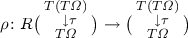• is an Eilenberg-Moore $R$-algebra, that is also called a modality. It is further subject to the monotonicity condition that is much like in Definition 2.2: the map

  

  is monotone for each algebra $a$. Here the order of each homset is induced by the enrichment of $\mathcal {K}{}\ell (T)$ via $\mathcal {E}{}\mathcal {M}(T)(b,\tau ) \mathop {\rightarrow }\limits ^{U^{T}} \mathbb {C}(U^{T}b,T\varOmega ) = \mathcal {K}{}\ell (T)(U^{T}b,\varOmega )$.

The situation is as in the following diagram.

(14)

The composite adjunction yields a new monad $U^{T}U^{R}F^{R}F^{T}=U^{T}R F^{T}$ on $\mathbb {C}$; then from the Kleisli category ${\mathcal {K}{}\ell (U^{T}R F^{T})}$ for the new monad we obtain a comparison functor to $\mathcal {E}{}\mathcal {M}(R)$. It is denoted by $K$.

We have a monad $R$ on $\mathcal {E}{}\mathcal {M}(T)$ and an algebra (modality) $\rho$ for it. This is much like in the original notion of PT situation, where $\tau :T(T\varOmega )\rightarrow T\varOmega$ is a modality from which we derived a weakest precondition semantics. Indeed, the following construction is parallel to Proposition 2.9.

Proposition 4.2

(the indexed poset $\mathbb {P}^{\mathcal {E}{}\mathcal {M}}(\tau ,\rho )$ ). A 2-player PT situation $(T,\varOmega ,\tau ,R,\rho )$ induces an indexed poset $\mathbb {P}^{\mathcal {E}{}\mathcal {M}}(\tau ,\rho ):\mathcal {E}{}\mathcal {M}(R)^{\mathop {\mathrm {op}}\nolimits } \rightarrow \mathbf {Posets}$ over $\mathcal {E}{}\mathcal {M}(T)$ by:

• on an object $\alpha \in \mathcal {E}{}\mathcal {M}(R)$,

  

  where the order $\sqsubseteq$ on the set $\mathcal {E}{}\mathcal {M}(R)(\alpha ,\rho )$ is inherited from $\mathbb {C}(X,T\varOmega )$ via the forgetful functors $\mathcal {E}{}\mathcal {M}(R)\rightarrow \mathcal {E}{}\mathcal {M}(T)\rightarrow \mathbb {C}$; and

• on an arrow ,

  

Proof

The same as the proof of Proposition 2.9, relying on Lemma 2.8.    $\square$

Much like in Theorem 2.10, composition of the indexed poset $\mathbb {P}^{\mathcal {E}{}\mathcal {M}}(\tau ,\rho ): \mathcal {E}{}\mathcal {M}(R)^{\mathop {\mathrm {op}}\nolimits }\rightarrow \mathbf {Posets}$ and the comparison functor $K:\mathcal {K}{}\ell (U^{T}R F^{T})\rightarrow \mathcal {E}{}\mathcal {M}(R)$ will yield the weakest precondition calculus. The branching computations of our interest are therefore of the type $X\rightarrow U^{T}R F^{T} Y$. We will later see, through examples, that this is indeed what models the scenarios in Sect. 3.

Note that in what follows we rely heavily on the adjunction $F^{T}\dashv U^{T}$.

Proposition 4.3

(the indexed poset $\mathbb {P}^{\mathcal {K}{}\ell }(\tau ,\rho )$ ). A 2-player PT situation $(T,\varOmega ,\tau ,R,\rho )$ induces an indexed poset $\mathbb {P}^{\mathcal {K}{}\ell }(\tau ,\rho ):\mathcal {K}{}\ell (U^{T}R F^{T})^{\mathop {\mathrm {op}}\nolimits } \rightarrow \mathbf {Posets}$ by:

• on an object $X\in \mathcal {K}{}\ell (U^{T}R F^{T})$, $\mathbb {P}^{\mathcal {K}{}\ell }(\tau ,\rho )(X):=\mathcal {K}{}\ell (T)(X,\varOmega )=\mathbb {C}(X,T\varOmega )$;

• given an arrow in $\mathcal {K}{}\ell (U^{T}R F^{T})$, it induces an arrow $f^{\wedge }:F^{T}X\rightarrow R(F^{T}Y)$ in $\mathcal {E}{}\mathcal {M}(T)$; this is used in

  $$\begin{aligned} \mathcal {E}{}\mathcal {M}(T)(F^{T}Y,\tau ) \rightarrow \mathcal {E}{}\mathcal {M}(T)(F^{T}X,\tau )\,, \quad q\longmapsto \bigl ( F^{T}X\mathop {\rightarrow }\limits ^{f^{\wedge }} R (F^{T}Y)\mathop {\rightarrow }\limits ^{R q} R\tau \mathop {\rightarrow }\limits ^{\rho } \tau \bigr ) \,. \end{aligned}$$

  The last map defines an arrow $\mathbb {P}^{\mathcal {K}{}\ell }(\tau ,\rho )(f):\mathbb {P}^{\mathcal {K}{}\ell }(\tau ,\rho )(Y)\rightarrow \mathbb {P}^{\mathcal {K}{}\ell }(\tau ,\rho )(X)$ since we have $\mathbb {P}^{\mathcal {K}{}\ell }(\tau ,\rho )(U) = \mathbb {C}(U,T\varOmega ) \cong \mathcal {E}{}\mathcal {M}(T)(F^{T}U,\tau )$.

We have the following natural isomorphism, where $K$ is the comparison in (14).

(15)

Proof

Note here that the comparison functor $K$ is concretely described as follows: $KX=F^{R}(F^{T}X)$ on objects, and use the correspondence

$$\begin{aligned} \mathcal {K}{}\ell (U^{T}R F^{T})(X,Y)&= \mathbb {C}(X, U^{T}U^{R}F^{R}F^{T}Y) \cong \mathcal {E}{}\mathcal {M}(T)(F^{T}X, U^{R}F^{R}F^{T}Y)\\&\ \ \ \ \ \ \,\, \cong \mathcal {E}{}\mathcal {M}(R)(F^{R}F^{T}X, F^{R}F^{T}Y) = \mathcal {E}{}\mathcal {M}(R)(KX, KY) \end{aligned}$$

for its action on arrows. We claim that the desired natural isomorphism $\varXi \mathbin {\bullet }\varPsi$ is the (vertical) composite

$$\begin{aligned} \mathbb {P}^{\mathcal {K}{}\ell }(\tau ,\rho ) (X)&= \mathbb {C}(X,T\varOmega ) \mathop {\longrightarrow }\limits ^{\varPsi _{X}} \mathcal {E}{}\mathcal {M}(T)(F^{T}X,\tau ) \\&\ \ \ \ \ \ \ \ \ \ \ \ \ \ \ \ \ \ \ \ \ \ \ \ \ \ \quad \,\,\mathop {\longrightarrow }\limits ^{\varXi _{X}} \mathcal {E}{}\mathcal {M}(R)(F^{R}F^{T}X,\rho ) = \mathbb {P}^{\mathcal {E}{}\mathcal {M}}(\tau ,\rho ) (KX) \end{aligned}$$

where $\varPsi$ and $\varXi$ are isomorphisms induced by adjunctions.

We have to check that $\varPsi _{X}$ and $\varXi _{X}$ are order isomorphisms. The map $\varPsi _{X}$ is monotone due to the monotonicity condition on $\tau$ (Definition 2.2); so is $\varPsi _{X}^{-1}$ by Lemma 2.8. Similarly, $\varXi _{X}$ is monotone by the monotonicity condition on $\rho$ (Definition 4.1); so is $\varXi _{X}^{-1}$ by Lemma 2.8.

We turn to the naturality: the following diagram must be shown to commute, for each in $\mathcal {K}{}\ell (U^{T}R F^{T})$.

(16)

The square on the left commutes by the definition of $\mathbb {P}^{\mathcal {K}{}\ell }(\tau ,\rho )(f)$ (Proposition 4.3); the one on the right is much like the one in (9) and its commutativity can be proved in the same way. Note here that $Kf=\mu ^{R}_{F^{T}Y}\mathrel {\circ }R (f^{\wedge })$.

Since the diagram (16) commutes, and since $\varPsi$ and $\varXi$ are order isomorphisms and $\mathbb {P}^{\mathcal {E}{}\mathcal {M}}(\tau ,\rho )(Kf)$ is monotone (Proposition 4.2), we have that $\mathbb {P}^{\mathcal {K}{}\ell }(\tau ,\rho )f$ is monotone. The functoriality of $\mathbb {P}^{\mathcal {K}{}\ell }(\tau ,\rho )$ is easy, too. This concludes the proof.    $\square$

5 Examples of 2-Player PT Situations

5.1 Nondeterministic Player and then Nondeterministic Opponent

We continue Sect. 3 and locate the monad $\mathcal {U{}P}$—and the logic of forced predicates—in the general setup of Sect. 4. We identify a suitable 2-player PT situation $(\mathcal P,1,\tau _{\Box },\mathsf {R}_{\mathsf {G}},\rho _{\mathsf {P}})$, in which $T=\mathcal P$, $\varOmega =1$ and $\tau =\tau _{\Box }$ that is from Sect. 2.3. The choice of $\tau _{\Box }$ corresponds to the demonic nature of Opponent’s choices: Player can force those properties that hold whatever choices Opponent makes.

To introduce the monad $\mathsf {R}_{\mathsf {G}}$ on $\mathcal {E}{}\mathcal {M}(\mathcal P)$—corresponding to the up-closed powerset construction—we go via the following standard isomorphism.

Lemma 5.1

Let $C:\mathcal {E}{}\mathcal {M}(\mathcal P)\rightarrow \mathbf {CL}_{\bigwedge }$ be the functor such that , where the order is defined by $x\sqsubseteq _{a} y$ if $x=a\{x,y\}$. Conversely, let $D:\mathbf {CL}_{\bigwedge }\rightarrow \mathcal {E}{}\mathcal {M}(\mathcal P)$ be such that . Both act on arrows as identities.

Then $C$ and $D$ constitute an isomorphism .    $\square$

The monad $\mathsf {R}_{\mathsf {G}}$ is then defined to be the composite $\mathsf {R}_{\mathsf {G}}:=D\mathrel {\circ }\mathsf {Dw}\mathrel {\circ }C$, using the down-closed powerset monad $\mathsf {Dw}$ on $\mathbf {CL}_{\bigwedge }$.

(17)

The switch between up-closed subsets in $\mathcal {U{}P}$ and down-closed subsets $\mathsf {Dw}$ may seem confusing. Later in Proposition 5.3 it is shown that everything is in harmony; and after all it is a matter of presentation since there is an isomorphism that reverses the order in each complete lattice. The switch here between up- and down-closed is essentially because: the bigger the set of Opponent’s options is, the smaller the power of Player (to force Opponent to somewhere) is.

Concretely, the monad $\mathsf {Dw}:\mathbf {CL}_{\bigwedge }\rightarrow \mathbf {CL}_{\bigwedge }$ carries a complete lattice $(X,\sqsubseteq )$ to the set $\mathsf {Dw}X := \{S\subseteq X\mid x\sqsubseteq x',\, x'\in S\Rightarrow x\in S\}$. We equip $\mathsf {Dw}X$ with the inclusion order; this makes $\mathsf {Dw}X$ a complete lattice, with sups and infs given by unions and intersections, respectively. An arrow $f:X\rightarrow Y$ is carried to $\mathsf {Dw}f:\mathsf {Dw}X\rightarrow \mathsf {Dw}Y$ defined by $S\mapsto \mathop {\downarrow }\nolimits (\mathop {\amalg }\nolimits _{f}S)$. Here $\mathop {\downarrow }\nolimits (\underline{}\,)$ denotes the downward closure and it is needed to ensure down-closedness (consider a $\bigwedge$-preserving map $f:1\rightarrow 2$, $0\mapsto 1$ where $0\sqsubseteq 1$ in $2$). The monad structure of $\mathsf {Dw}$ is given by: $\eta ^{\mathsf {Dw}}_{X}:X\rightarrow \mathsf {Dw}X, x\mapsto \mathop {\downarrow }\nolimits \{x\}$; and $\mu ^{\mathsf {Dw}}_{X}:\mathsf {Dw}(\mathsf {Dw}X)\rightarrow \mathsf {Dw}X, \mathfrak {a}\mapsto \bigcup \mathfrak {a}$. Note in particular that $\eta ^{\mathsf {Dw}}_{X}$ is $\bigwedge$-preserving. As in (17) we define $\mathsf {R}_{\mathsf {G}}:=D\mathrel {\circ }\mathsf {Dw}\mathrel {\circ }C$.

Finally, let us define the data $\rho _{\mathsf {P}}:\mathsf {R}_{\mathsf {G}}(\tau _{\Box })\rightarrow \tau _{\Box }$ in the 2-player PT situation. Via the isomorphism (17) we shall think of it as an $\mathsf {Dw}$-algebra, where the $\mathcal P$-algebra $\tau _{\Box }$ is identified with the 2-element complete lattice $[\mathtt {f{}f}\sqsubseteq \mathtt {t{}t}]$ (the order is because $\tau _{\Box }\{\mathtt {t{}t},\mathtt {f{}f}\}=\mathtt {f{}f}$). Therefore we are looking for a $\bigwedge$-preserving map

$$\begin{aligned} \mathsf {Dw}[\mathtt {f{}f}\sqsubseteq \mathtt {t{}t}] \,=\,\bigl [\,\emptyset \sqsubseteq \{\mathtt {f{}f}\}\sqsubseteq \{\mathtt {f{}f},\mathtt {t{}t}\}\,\bigr ] \;\mathop {\longrightarrow }\limits ^{C\rho _{\mathsf {P}}}\; [\mathtt {f{}f}\sqsubseteq \mathtt {t{}t}] \end{aligned}$$

subject to the conditions of an Eilenberg-Moore algebra in (4). In fact such $C(\rho _{\mathsf {P}})$ is uniquely determined: preservation of $\top$ forces $(C\rho _{\mathsf {P}})\{\mathtt {f{}f},\mathtt {t{}t}\}=\mathtt {t{}t}$; the unit law forces $(C\rho _{\mathsf {P}})\{\mathtt {f{}f}\}=\mathtt {f{}f}$ and monotonicity of $C\rho _{\mathsf {P}}$ then forces $(C\rho _{\mathsf {P}})\emptyset =\mathtt {f{}f}$.

Lemma 5.2

$(\mathcal P,1, \tau _{\Box }, \mathsf {R}_{\mathsf {G}}, \rho _{\mathsf {P}})$ thus obtained is a 2-player PT situation.

Proof

It remains to check the monotonicity condition (Definition 4.1) for $\rho _{\mathsf {P}}$. We shall again think in terms of complete lattices and $\bigwedge$-preserving maps; then the requirement is that the map $\bigl (X\mathop {\rightarrow }\limits ^{f}[\mathtt {f{}f}\sqsubseteq \mathtt {t{}t}]\bigr ) \mapsto \bigl ( \mathsf {Dw}X\mathop {\rightarrow }\limits ^{\rho _{\mathsf {P}}\mathrel {\circ }\mathsf {Dw}f} [\mathtt {f{}f}\sqsubseteq \mathtt {t{}t}] \bigr )$ is monotone. Assume $g\sqsubseteq f$, $S\in \mathsf {Dw}X$ and $(\rho _{\mathsf {P}}\mathrel {\circ }\mathsf {Dw}f)(S)=\mathtt {f{}f}$. It suffices to show that $(\rho _{\mathsf {P}}\mathrel {\circ }\mathsf {Dw}g)(S)=\mathtt {f{}f}$; this follows from the observation that, for $h=f$ or $g$,

   $\square$

Let us check that the logic $\mathbb {P}^{\mathcal {K}{}\ell }(\tau _{\Box },\rho _{\mathsf {P}})$ associated with this 2-player PT situation is indeed the logic of forced predicates in Sect. 3.1. For instance, we want “computations” $X\rightarrow U^{\mathcal P}\mathsf {R}_{\mathsf {G}}F^{\mathcal P}Y$ to coincide with “computations” $X\rightarrow \mathcal {U{}P}Y$.

Proposition 5.3

For any set $X$ we have $U^{\mathcal P}\mathsf {R}_{\mathsf {G}}F^{\mathcal P}= \mathcal {U{}P}X$. In fact they are isomorphic as complete lattices, that is, $\mathsf {Dw}\mathrel {\circ }C\mathrel {\circ }F^{\mathcal P} = \mathcal {U{}P}:\mathbf {Sets}\rightarrow \mathbf {CL}_{\bigwedge }$ where the functor $\mathcal {U{}P}$ is equipped with the inclusion order.

Proof

Given $X\in \mathbf {Sets}$, the definition of $C$ dictates that $C(F^{\mathcal P} X)=(\mathcal PX,\supseteq )$ and its order be given by the reverse inclusion order. Hence $\mathsf {Dw}(C(F^{\mathcal P} X))$ is the collection of families $\mathfrak {a}\subseteq \mathcal PX$ that are $\supseteq$-down-closed, i.e. $\subseteq$-up-closed. It is easily checked that the two functors coincide on arrows, too, using the characterization on the left in (13).    $\square$

Next we describe the logic $\mathbb {P}^{\mathcal {K}{}\ell }(\tau _{\Box },\rho _{\mathsf {P}})$ (Proposition 4.3) in concrete terms. We base ourselves again in $\mathbf {CL}_{\bigwedge }$ via the isomorphism $\mathcal {E}{}\mathcal {M}(\mathcal P)\cong \mathbf {CL}_{\bigwedge }$ in (17). Consider a postcondition $q:Y\rightarrow \mathcal P1$ and a branching computation $f:X\rightarrow \mathcal {U{}P}Y$. These are in one-to-one correspondences with the following arrows in $\mathbf {CL}_{\bigwedge }$:

$$\begin{aligned} q^{\wedge }&:\; C(F^{\mathcal P} Y) = (\mathcal PY, \supseteq ) \longrightarrow [\mathtt {f{}f}\sqsubseteq \mathtt {t{}t}] = C(\tau _{\Box })\,, \\ f^{\wedge }&:\; C(F^{\mathcal P} X) = (\mathcal PX, \supseteq ) \longrightarrow \mathsf {Dw}(\mathcal PY,\supseteq ) = C(\mathsf {R}_{\mathsf {G}}(F^{\mathcal P} Y))\,, \end{aligned}$$

where we used Proposition 5.3. Since $q^{\wedge }$ are $f^{\wedge }$ are $\bigwedge$-preserving, we have

$$\begin{aligned}\textstyle q^{\wedge }W = q^{\wedge }(\bigcup _{y\in W}\{y\}) = q^{\wedge }(\bigwedge _{y\in W}\{y\}) = \bigwedge _{y\in W} q^{\wedge }\{y\} = \bigwedge _{y\in W} qy\,; \end{aligned}$$

and similarly $f^{\wedge }S=\bigcap _{x\in S}fx$. Recall that $\mathsf {Dw}(\mathcal PY,\supseteq )$ has the inclusion order.

Now Proposition 4.3 states that the weakest precondition $\mathbb {P}^{\mathcal {K}{}\ell }(\tau _{\Box },\rho _{\mathsf {P}})(f)(q)$ is the arrow $X\rightarrow \mathcal P1$ that corresponds, via the adjunction $C\mathrel {\circ }F^{\mathcal P}\dashv U^{\mathcal P}\mathrel {\circ }D$, to

$$\begin{aligned} (\mathcal PX, \supseteq ) \mathop {\longrightarrow }\limits ^{f^{\wedge }} \mathsf {Dw}(\mathcal PY,\supseteq ) \mathop {\longrightarrow }\limits ^{\mathsf {Dw}(q^{\wedge })} \mathsf {Dw}[\mathtt {f{}f}\sqsubseteq \mathtt {t{}t}] \mathop {\longrightarrow }\limits ^{\rho _{\mathsf {P}}} [\mathtt {f{}f}\sqsubseteq \mathtt {t{}t}] \quad \mathrm{in} \mathbf {CL}_{\bigwedge }. \end{aligned}$$

Unweaving definitions it is straightforward to see that, for $S\subseteq X$,

$$\begin{aligned}&\bigl (\rho _{\mathsf {P}}\mathrel {\circ }\mathsf {Dw}(q^{\wedge })\mathrel {\circ }f^{\wedge }\bigr ) S =\mathtt {t{}t}\;\Longleftrightarrow \; \exists W\subseteq Y.\, \bigl ( \forall x\in S.\, W\in fx \wedge \forall y\in W.\, qy=\mathtt {t{}t}\bigr )\,; \nonumber \\&\text {therefore } \mathbb {P}^{\mathcal {K}{}\ell }(\tau _{\Box },\rho _{\mathsf {P}})(f)(q)(x) =\mathtt {t{}t}\;\Longleftrightarrow \; \exists W\subseteq Y.\, \bigl ( W\in fx \wedge \forall y\in W.\, qy=\mathtt {t{}t}\bigr )\,. \end{aligned}$$

(18)

The last condition reads: among the set $fx$ of possible moves of Player, there exists a move $W$, from which $q$ holds no matter what Opponent’s move $y$ is. Therefore $\mathbb {P}^{\mathcal {K}{}\ell }(\tau _{\Box },\rho _{\mathsf {P}})(f)(q)(x)=\mathtt {t{}t}$ if Player can force the predicate $q$ from $x$ after the (two-layer branching) computation $f$.

5.2 Nondeterministic Opponent and then Nondeterministic Player

We change the order of Player and Opponent: $\mathsf {O}$ moves first and then $\mathsf {P}$ moves. The general setup in Sect. 4 successfully models this situation too, with a choice of a 2-player PT situation $(\mathcal P, 1, \tau _{\Diamond },\mathsf {R}_{\mathsf {G}}, \rho _{\mathsf {O}})$ that is dual to the previous one.

The modality $\tau _{\Diamond }$ is from Sect. 2.3. Although the monad $\mathsf {R}_{\mathsf {G}}$ is the same as in Sect. 5.1, we now prefer to present it in terms of $\mathcal {E}{}\mathcal {M}(\mathcal P)\cong \mathbf {CL}_{\bigvee }$ instead of $\mathbf {CL}_{\bigwedge }$. The reason is that this way the algebra $\tau _{\Diamond }$ gets identified with $[\mathtt {f{}f}\sqsubseteq \mathtt {t{}t}]$, which is intuitive. The situation is as follows.

(19)

The functors $C''$ and $D''$ carries a complete lattice $(X,\sqsubseteq )$ to $(X,\sqsupseteq )$, reversing the order. The monad $\mathsf {Up}$ is defined by $\mathsf {Up}:=C''\mathrel {\circ }\mathsf {Dw}\mathrel {\circ }D''$; concretely it carries $(X,\sqsubseteq )$ to the set of its up-closed subsets, equipped with the reverse inclusion order $\supseteq$. That is,

$$\begin{aligned} \mathsf {Up}(X,\sqsubseteq ) \;:=\; \bigl (\, \{S\subseteq X\mid S\ni x\sqsubseteq x'\Rightarrow x'\in S\} \,,\; \supseteq \,\bigr )\,. \end{aligned}$$

We have $\mathsf {R}_{\mathsf {G}}=D\mathrel {\circ }\mathsf {Dw}\mathrel {\circ }C=D'\mathrel {\circ }\mathsf {Up}\mathrel {\circ }C'$.

The modality $\rho _{\mathsf {O}}:\mathsf {R}_{\mathsf {G}}(\tau _{\Diamond })\rightarrow \tau _{\Diamond }$ is identified, via the isomorphism $C'$ in (19), with an $\mathsf {Up}$-algebra on $[\mathtt {f{}f}\sqsubseteq \mathtt {t{}t}]$. The latter is a $\bigvee$-preserving map

$$\begin{aligned} \mathsf {Up}[\mathtt {f{}f}\sqsubseteq \mathtt {t{}t}] = \bigl [\,\{\mathtt {f{}f},\mathtt {t{}t}\}\sqsubseteq \{\mathtt {t{}t}\}\sqsubseteq \emptyset \,\bigr ] \;\mathop {\longrightarrow }\limits ^{C'\rho _{\mathsf {O}}}\; [\mathtt {f{}f}\sqsubseteq \mathtt {t{}t}]\,; \end{aligned}$$

note here that the order in $\mathsf {Up}(X,\sqsubseteq )$ is the reverse inclusion $\supseteq$. Such $C'\rho _{\mathsf {O}}$ is uniquely determined (as before): the unit law forces $(C'\rho _{\mathsf {O}})\{\mathtt {t{}t}\}=\mathtt {t{}t}$; preservation of $\bot$ forces $(C'\rho _{\mathsf {O}})\{\mathtt {t{}t},\mathtt {f{}f}\}=\mathtt {f{}f}$; and then by monotonicity $(C'\rho _{\mathsf {O}})\emptyset =\mathtt {t{}t}$.

It is straightforward to see that $(\mathcal P,1,\tau _{\Diamond },\mathsf {R}_{\mathsf {G}},\rho _{\mathsf {O}})$ is indeed a 2-player PT situation; the proof is symmetric to the one in Sect. 5.1. Also symmetrically, the weakest precondition semantics $\mathbb {P}^{\mathcal {K}{}\ell }(\tau _{\Diamond },\rho _{\mathsf {O}})$ is concretely described as follows: given a postcondition $q:Y\rightarrow \mathcal P1$ and a branching computation $f:X\rightarrow \mathcal {U{}P}Y$,

$$\begin{aligned} \mathbb {P}^{\mathcal {K}{}\ell }(\tau _{\Diamond },\rho _{\mathsf {O}})(f)(q)(x) =\mathtt {t{}t}\;\Longleftrightarrow \; \forall W\subseteq Y.\, \bigl ( W\in fx \Rightarrow \exists y\in W.\, qy=\mathtt {t{}t}\bigr )\,. \end{aligned}$$

This is dual to (18) and reads: whatever move $W$ Opponent takes, there exists Player’s move $y\in W$ so that $q$ holds afterwards.

We note that the analogue of Proposition 5.3 becomes: $\mathsf {Up}\mathrel {\circ }C'\mathrel {\circ }F^{\mathcal P}=\mathcal {U{}P}:\mathbf {Sets}\rightarrow \mathbf {CL}_{\bigvee }$, where each $\mathcal {U{}P}X$ is equipped with the reverse inclusion order. This order ($\mathfrak {a}\sqsubseteq \mathfrak {b}$ in $\mathcal {U{}P}X$ if $\mathfrak {a}\supseteq \mathfrak {b}$) is intuitive if we think of $\sqsubseteq$ as the power of Player.

Remark 5.4

The constructions have been described in concrete terms; this is for intuition. An abstract view is possible too: the modality $\tau _{\Diamond }$ is the dual of $\tau _{\Box }$ via the swapping $\sigma$ (see (7)); and the other modality $\rho _{\mathsf {O}}$ is also the dual of $\rho _{\mathsf {P}}$ by $\rho _{\mathsf {O}}= \bigl (\, \mathsf {R}_{\mathsf {G}}(\tau _{\Diamond }) \mathop {\rightarrow }\limits ^{\mathsf {R}_{\mathsf {G}}\sigma } \mathsf {R}_{\mathsf {G}}(\tau _{\Box }) \mathop {\rightarrow }\limits ^{\rho _{\mathsf {P}}} \tau _{\Box }\mathop {\rightarrow }\limits ^{\sigma } \tau _{\Diamond }\,\bigr )$.

5.3 Nondeterministic Opponent and then Probabilistic Player

In our last example Opponent $\mathsf {O}$ moves nondeterministically first, and then Player $\mathsf {P}$ moves probabilistically. Such nested branching is in many process-theoretic models of probabilistic systems (see Sect. 3, in particular Sect. 3.2), most notably in Segala’s probabilistic automata [27]. We identify a 2-player PT situation $(\mathcal D\!, 1, \tau _{\mathrm {total}}, \mathcal {C}{}v,\rho _{\mathrm {inf}})$ for this situation; then the associated logic $\mathbb {P}^{\mathcal {K}{}\ell }(\tau _{\mathrm {total}},\rho _{\mathrm {inf}})$ is that of the probabilistic predicate transformers in [31]. The modality $\tau _{\mathrm {total}}$ is from Sect. 2.3. The other components ($\mathcal {C}{}v$, $\rho _{\mathrm {inf}}$) are to be described in terms of convex cones and their convex subsets.

In what follows a $\mathcal D\!$-algebra is referred to as a convex cone, adopting the notation $\sum _{i\in I}w_{i}x_{i}$ to denote $a\bigl (\,[x_{i}\mapsto w_{i}]_{i\in I}\,\bigr )\in X$ in a convex cone $a:\mathcal D\!X\rightarrow X$. Here $I$ is a countable index set,³ $w_{i}\in [0,1]$, and $\sum _{i\in I}w_{i}\le 1$. Note that, since $\mathcal D\!$ is the subdistribution monad, the zero distribution $\mathbf {0}$ is allowed in $\mathcal D\!X$ and therefore a convex cone $a:\mathcal D\!X\rightarrow X$ has its apex $a\mathbf {0}\in X$. Similarly, a morphism of $\mathcal D\!$-algebras is referred to as a convex linear map.

Definition 5.5

(convex subset). A subset $S\subseteq X$ of a convex cone $a:\mathcal D\!X\rightarrow X$ is said to be convex if, for any $p_{i}\in [0,1]$ such that $\sum _{i\in I}p_{i}=1$ and any $x_{i}\in S$, the convex combination $\sum _{i\in I}p_{i}x_{i}$ belongs to $S$.

We emphasize that in the last definition $\sum _{i}p_{i}$ is required to be $=1$. This is unlike $\sum _{i}w_{i}\le 1$ in the definition of convex cone. Therefore a convex subset $S$ need not include the apex $a\mathbf {0}$; one can think of the base of a 3-dimensional cone as an example. This variation in the definitions is also found in [34, Sect. 2.1.2]; one reason is technical: if we allow $\sum _{i}p_{i}\le 1$ then it is hard to find the monad unit of $\mathcal {C}{}v$ (see below). Another process-theoretic reason is described later in Remark 5.8.

Definition 5.6

(the monad $\mathcal {C}{}v$ ). The functor $\mathcal {C}{}v:\mathcal {E}{}\mathcal {M}(\mathcal D\!)\rightarrow \mathcal {E}{}\mathcal {M}(\mathcal D\!)$ carries a convex cone $a:\mathcal D\!X\rightarrow X$ to $\mathcal {C}{}vX:=\{S\subseteq X\mid \text {S is convex}\}$; the latter is a convex cone by

$$\begin{aligned} \textstyle \sum _{i}w_{i}S_{i} \;:=\; \{\,\sum _{i}w_{i}x_{i}\mid x_{i}\in S_{i}\,\}\,. \end{aligned}$$

It is easy to see that $\sum _{i}w_{i}S_{i}$ is indeed a convex subset of $X$. Given a convex linear map $f:X\rightarrow Y$, $\mathcal {C}{}vf:\mathcal {C}{}vX\rightarrow \mathcal {C}{}vY$ is defined by $(\mathcal {C}{}vf)S:=\mathop {\amalg }\nolimits _{f}S$, which is obviously convex in $Y$, too.

The monad structure of $\mathcal {C}{}v$ is as follows. Its unit is $\eta ^{\mathcal {C}{}v}_{X}:=\{\underline{}\,\}:X\rightarrow \mathcal {C}{}vX$; note that a singleton $\{x\}$ is a convex subset of $X$ (Definition 5.5). The monad multiplication is $\mu ^{\mathcal {C}{}v}_{X}:=\bigcup :\mathcal {C}{}v(\mathcal {C}{}vX)\rightarrow \mathcal {C}{}vX$. It is easy to see that $\eta ^{\mathcal {C}{}v}_{X}$ and $\mu ^{\mathcal {C}{}v}_{X}$ are convex linear maps, and that they satisfy the monad axioms.

We introduce the last component, namely the modality $\rho _{\mathrm {inf}}:\mathcal {C}{}v(\tau _{\mathrm {total}})\rightarrow \tau _{\mathrm {total}}$. A convex subset $S$ of the carrier $\mathcal D\!1=[0,1]$ of $\tau _{\mathrm {total}}$ is nothing but an interval (its endpoints may or may not be included); $\rho _{\mathrm {inf}}$ then carries such $S$ to its infimum $\inf S\in [0,1]$. That $\rho _{\mathrm {inf}}$ is convex linear, and that it satisfies the Eilenberg-Moore axioms, are obvious.

Much like in Lemma 5.2, we obtain:

Lemma 5.7

$(\mathcal D\!,1, \tau _{\mathrm {total}}, \mathcal {C}{}v, \rho _{\mathrm {inf}})$ thus obtained is a 2-player PT situation.    $\square$

The resulting logic $\mathbb {P}^{\mathcal {K}{}\ell }(\tau _{\mathrm {total}},\rho _{\mathrm {inf}})$ is as follows. Given a postcondition $q:Y\rightarrow \mathcal D\!1$ and a computation $f:X\rightarrow U^{\mathcal D\!}\mathcal {C}{}vF^{\mathcal D\!} Y$, the weakest precondition is

$$\begin{aligned} \textstyle \mathbb {P}^{\mathcal {K}{}\ell }(\tau _{\mathrm {total}},\rho _{\mathrm {inf}})(f)(q)(x) \;=\; \inf \bigl \{\,\sum _{y\in Y} d(y)\cdot q(y)\,\bigl |\bigr .\, d\in f(x)\,\bigr \} \,. \end{aligned}$$

(20)

Here $d$ is a subdistribution chosen by Opponent; and the value $\sum _{y\in Y} d(y)\cdot q(y)$ is the expected value of the random variable $q$ under the distribution $d$. Therefore the weakest precondition computed above is the least expected value of $q$ when Opponent picks a distribution in harm’s way. This is the same as in [31].

Remark 5.8

The use of the convex powerset construction, instead of (plain) powersets, was motivated in Sect. 3.2 through the technical difficulty in getting a monad. Convex powersets are commonly used in the process-theoretic study of probabilistic systems, also because they model a probabilistic scheduler: Opponent (called a scheduler in this context) can not only pick one distribution but also use randomization in doing so. See e.g. [2].

The definition of convex subset (Definition 5.5)—where we insist on $\sum _{i}p_{i}=1$ instead of $\le 1$—is natural in view of the logic $\mathbb {P}^{\mathcal {K}{}\ell }(\tau _{\mathrm {total}},\rho _{\mathrm {inf}})$ described above. Relaxing this definition entails that the zero distribution $\mathbf {0}$ is always included in a “convex subset,” and hence always in Opponent’s options. This way, however, the weakest precondition in (20) can always be forced to $0$ and the logic gets trivial.

We can also model the situation where the roles of Player and Opponent are swapped: we can follow the same path as in Remark 5.4 and obtain a 2-player PT situation $(\mathcal D\!, 1, \tau _{\mathrm {partial}}, \mathcal {C}{}v, \rho _{\mathrm {sup}})$; the resulting modality $\rho _{\mathrm {sup}}$ carries an interval to its supremum.

6 Conclusions and Future Work

Inspired by Jacobs’ recent work [16, 17] we pursued a foundation of predicate transformers (more specifically weakest precondition semantics) based on an order-enriched monad. There different notions of modality (such as “may” vs. “must”) are captured by Eilenberg-Moore algebras. Nested branching with two conflicting players can be modeled in a modular way, too, by a monad $R$ on an Eilenberg-Moore category $\mathcal {E}{}\mathcal {M}(T)$. Instances of this generic framework include probabilistic weakest preconditions, those augmented with nondeterminism, and the logic of forced predicates in games.

As future work we wish to address the components in the picture (2–3) that are missing in the current framework. A generic weakest precondition calculus presented in a syntactic form is another direction. Most probably relationships between monads and algebraic theories (see e.g. [32]) will be exploited there. So-called healthiness conditions—i.e. characterization of the image of $\mathbb {P}^{\mathcal {K}{}\ell }(\tau )$ in (8), to be precise its action on arrows—are yet another topic, generalizing [5, 31].

The current work is hopefully a step forward towards a coalgebraic theory of automata (on infinite trees), games and fixed-point logics. For example, we suspect that our categorical formulation of the logic of forced predicates be useful in putting game (bi)simulation (studied e.g. in [22, 36]) in coalgebraic terms. Possibly related, we plan to work on the relationship to the coalgebraic theory of traces and simulations formulated in a Kleisli category [11, 13] since all the monads in Example 2.2 fit in this trace framework.

In this paper we relied on an order-enrichment of a monad to obtain the entailment order. We are nevertheless interested in what our current framework brings for other monads, like the ones that model computational effects [29] (global state, I/O, continuation, etc.). Also interesting is a higher-order extension of the current work, where the logic will probably take the form of dependent types. Related work in this direction is [20].

References

Barr, M., Wells, C.: Toposes, Triples and Theories. Springer, Berlin (1985)
Cattani, S., Segala, R.: Decision algorithms for probabilistic bisimulation. In: Brim, L., Jančar, P., Křetínský, M., Kučera, A. (eds.) CONCUR 2002. LNCS, vol. 2421, pp. 371–385. Springer, Heidelberg (2002)
Cheung, L.: Reconciling nondeterministic and probabilistic choices. Ph.D. thesis, Radboud Univ. Nijmegen (2006)
Cîrstea, C.: A coalgebraic approach to linear-time logics. In: Muscholl, A. (ed.) FOSSACS 2014. LNCS, vol. 8412, pp. 426–440. Springer, Heidelberg (2014)
Dijkstra, E.W.: A Discipline of Programming. Prentice Hall, Upper Saddle River (1976)
Foulis, D.J., Bennett, M.K.: Effect algebras and unsharp quantum logics. Found. Physics 24(10), 1331–1352 (1994)
Giry, M.: A categorical approach to probability theory. In: Proceedings of the Categorical Aspects of Topology and Analysis. Lecture Notes in Mathematics, vol. 915, pp. 68–85 (1982)
Grädel, E., Thomas, W., Wilke, T. (eds.): Automata, Logics, and Infinite Games: A Guide to Current Research. LNCS, vol. 2500. Springer, Heidelberg (2002)
Hansen, H.H., Kupke, C.: A coalgebraic perspective on monotone modal logic. Electr. Notes Theor. Comput. Sci. 106, 121–143 (2004)
Hansen, H.H., Kupke, C., Pacuit, E.: Neighbourhood structures: Bisimilarity and basic model theory. Log. Methods Comput. Sci. 5(2), 1–32 (2009)
Hasuo, I.: Generic forward and backward simulations II: probabilistic simulation. In: Gastin, P., Laroussinie, F. (eds.) CONCUR 2010. LNCS, vol. 6269, pp. 447–461. Springer, Heidelberg (2010)
Hasuo, I., Hoshino, N.: Semantics of higher-order quantum computation via geometry of interaction. In: LICS. pp. 237–246. IEEE Computer Society (2011)
Hasuo, I., Jacobs, B., Sokolova, A.: Generic trace semantics via coinduction. Log. Methods Comput. Sci. 3(4:11), 1–36 (2007)
Hoare, C.A.R.: An axiomatic basis for computer programming. Commun. ACM, 12, 576–580, 583 (1969)
Jacobs, B.: Categorical Logic and Type Theory. North Holland, Amsterdam (1999)
Jacobs, B.: New directions in categorical logic, for classical, probabilistic and quantum logic. http://arxiv.org/abs/1205.3940
Jacobs, B.: Measurable spaces and their effect logic. In: LICS. pp. 83–92. IEEE Computer Society (2013)
Jones, C.: Probabilistic non-determinism. Ph.D. thesis, Univ. Edinburgh (1990)
Jurdziński, M.: Small progress measures for solving parity games. In: Reichel, H., Tison, S. (eds.) STACS 2000. LNCS, vol. 1770, pp. 290–301. Springer, Heidelberg (2000)
Katsumata, S.: Relating computational effects by \(\top \top \)-lifting. Inf. Comput. 222, 228–246 (2013)
Katsumata, S., Sato, T.: Preorders on monads and coalgebraic simulations. In: Pfenning, F. (ed.) FOSSACS 2013. LNCS, vol. 7794, pp. 145–160. Springer, Heidelberg (2013)
Kissig, C., Venema, Y.: Complementation of coalgebra automata. In: Kurz, A., Lenisa, M., Tarlecki, A. (eds.) CALCO 2009. LNCS, vol. 5728, pp. 81–96. Springer, Heidelberg (2009)
Kock, A.: Monads and extensive quantities (2011). arXiv:1103.6009
Kozen, D.: Semantics of probabilistic programs. J. Comput. Syst. Sci. 22(3), 328–350 (1981)
Kupke, C., Pattinson, D.: Coalgebraic semantics of modal logics: an overview. Theor. Comput. Sci. 412(38), 5070–5094 (2011)
Kupke, C., Venema, Y.: Coalgebraic automata theory: basic results. Log. Methods Comput. Sci. 4(4), 1–43 (2008)
Lynch, N.A., Segala, R., Vaandrager, F.W.: Compositionality for probabilistic automata. In: Amadio, R.M., Lugiez, D. (eds.) CONCUR 2003. LNCS, vol. 2761, pp. 208–221. Springer, Heidelberg (2003)
Lane, S.: Categories for the Working Mathematician, 2nd edn. Springer, Berlin (1998)
Moggi, E.: Notions of computation and monads. Inf. Comp. 93(1), 55–92 (1991)
Morgan, C.: Programming from Specifications. Prentice-Hall, London (1990)
Morgan, C., McIver, A., Seidel, K.: Probabilistic predicate transformers. ACM Trans. Program. Lang. Syst. 18(3), 325–353 (1996)
Plotkin, G., Power, J.: Adequacy for algebraic effects. In: Honsell, F., Miculan, M. (eds.) FOSSACS 2001. LNCS, vol. 2030, pp. 1–24. Springer, Heidelberg (2001)
Sokolova, A.: Coalgebraic analysis of probabilistic systems. Ph.D. thesis, Techn. Univ. Eindhoven (2005)
Tix, R., Keimel, K., Plotkin, G.D.: Semantic domains for combining probability and non-determinism. Elect. Notes Theor. Comput. Sci. 129, 1–104 (2005)
Varacca, D., Winskel, G.: Distributing probabililty over nondeterminism. Math. Struct. Comp. Sci. 16(1), 87–113 (2006)
Venema, Y., Kissig, C.: Game bisimulations between basic positions. Talk at Highlights of Logic, Games and Automata, Paris (2013)
Winskel, G.: The Formal Semantics of Programming Languages. MIT Press, Cambridge (1993)
Acknowledgments
Thanks are due to Kazuyuki Asada, Kenta Cho, Corina Cîrstea and Tetsuri Moriya for useful discussions. The author is supported by Grants-in-Aid for Young Scientists (A) No. 24680001, JSPS, and by Aihara Innovative Mathematical Modelling Project, FIRST Program, JSPS/CSTP.
Author information
Authors and Affiliations
Corresponding author
Editor information
Editors and Affiliations
Rights and permissions
Copyright information
© 2014 IFIP International Federation for Information Processing
About this paper
Cite this paper
Hasuo, I. (2014). Generic Weakest Precondition Semantics from Monads Enriched with Order. In: Bonsangue, M. (eds) Coalgebraic Methods in Computer Science. CMCS 2014. Lecture Notes in Computer Science(), vol 8446. Springer, Berlin, Heidelberg. https://doi.org/10.1007/978-3-662-44124-4_2
Download citation
DOI: https://doi.org/10.1007/978-3-662-44124-4_2
Published:
Publisher Name: Springer, Berlin, Heidelberg
Print ISBN: 978-3-662-44123-7
Online ISBN: 978-3-662-44124-4
eBook Packages: Computer ScienceComputer Science (R0)