The Emission Price Dynamics

Abstract

Since the creation of the European Union Emissions Trading Scheme (EU ETS) in 2005, a burgeoning academic literature has emerged to identify the key price drivers of European Union Allowances. This chapter overviews the main econometric studies that investigate energy prices, weather events, and macroeconomic shocks as determinants of allowance prices. A coal-to-gas switching model is introduced and calibrated to real data. Given the importance of understanding the emission permit price formation, this remaining of this chapter provides an overview of deterministic and stochastic equilibrium permit price models suggested in the literature. Several market design institutions are considered. Banking and borrowing limitations, strategic trading interactions, and asymmetric information in the permit market are the most relevant.

Appendix

This Appendix provides an overview of the techniques used to solve static and dynamic linear optimization problems and some details about the models introduced before.

6.1.1 Solving Static Optimization Problems

Definition 6.19

(Lagrangian)

Let $x = (x_{1}, \ldots, x_{n}) \in\mathbb{R}^{n}$ and let f(x),g ₁(x),…,g _m (x) be functions.

Then the Lagrangian of the following static nonlinear optimization problem

is given by

Definition 6.20

(Static convex optimization with non-negative control variables)

Let x=(x ₁,…,x _n′,x _n′+1,…,x _n ). Assume that f(x),g ₁(x),…,g _m (x) are convex functions that are continuously differentiable. Furthermore, assume that there exists $\tilde{x} \in\mathbb{R}^{n}$ such that $g_{j}(\tilde{x})< 0$ holds for all non-linear constraints. We consider the following optimization problem:

$$\everymath{\displaystyle} \begin{array}{l@{\quad}l@{\quad}l} \min_{x_1,\ldots,x_n}\bigl\{f(x)\bigr\}& \\ \text{subject to}& g_j(x) \leq0 &\text{for } j=1,\ldots,m \text{ and}\\ &x_i\geq0 &\text{for } i=1, \ldots, n'\ (n' \leq n). \end{array} $$

Theorem 6.21

(Karush–Kuhn–Tucker conditions)

$x=(\tilde{x}_{1},\ldots, \tilde{x}_{n})$ is the optimal solution of the optimization problem of Definition 6.20 if and only if there exists $\tilde{u}\in\mathbb{R}^{m}$ such that all the Karush–Kuhn–Tucker conditions are satisfied:

For i=1,…,n′

(A.1)

(A.2)

(A.3)

and for i=n′+1,…,n

(A.4)

and for j=1,…,m

(A.5)

(A.6)

(A.7)

6.1.2 Solving Dynamic Optimization Problems

Theorem 6.22

(Dynamic optimization problem)

Let T<∞ and let f and g be twice differentiable concave functions. Consider the following dynamic, deterministic optimization problem

(A.8)

(A.9)

(A.10)

(A.11)

Then the Hamiltonian is defined as

(A.12)

and the solution of the optimization problem must satisfy

(A.13)

(A.14)

(A.15)

(A.16)

Remark

• (a) x(t) is called control variable. The state variable s(t) is influenced by the choice of the control variable.

• (b) Equation (A.13) is similar to the condition in a static non-linear optimization problem.

• (c) Equation (A.15) restates the condition on the state variable (cf. Eq. (A.9)).

• (d) Equation (A.16) is called transversality condition.

Proof 9 (Idea)

A rigorous proof can be found in Pontryagin et al. (1962). The following proof is along the lines of Barro and Sala-i Martin (1995).

First, we rewrite the constraint as an integral and set up the Lagrangian function with the continuum of multipliers u(t) for the dynamic constraint and the multiplier v for the terminal condition of the state variable:

Second, integration by parts of

and using the definition of the Hamiltonian yields

(A.17)

Third, solve the problem using perturbation analysis:

Let $\bar{x}(t)$ be the optimal path for the control variable. The constraint $\dot{s}(t) = g (s(t), x(t), t )$ yields an optimal path for the state variable that we denote by $\bar{s}(t)$. Define the perturbations of the optimal paths by

where ε is a scalar and p ^(x):=p ^(x)(t) and p ^(s):=p ^(s)(t) are called perturbation functions. The perturbation analysis is completed by using that near the optimum small perturbations do not affect the maximum value of our optimization problem, that is,

(A.18)

Applying the chain rule to Eq. (A.17) yields

Since $\frac{\partial L}{\partial\varepsilon} (s(t),\bar{x}(t),t )=0$ must hold for any choice of perturbation functions, we obtain

Combining v=u(T) and v⋅s(T)=0, the complementary slackness condition from the terminal constraint, yields the so-called transversality condition

 □

6.1.3 Relationship Between Optimality Conditions

Lemma 6.23

A solution of the joint cost minimization problem satisfies the conditions of a market equilibrium.

Proof 10

Using the conditions given in (6.11) and (6.12) we show that

satisfy the conditions given in (6.7)–(6.10).

Conditions (6.11) and (6.12) imply Eq. (6.7):

Since $\frac{\partial C^{i}}{\partial Q^{i}}(\widetilde{Q}^{i})+\tilde{u}\leq0$ for and $\widetilde{Q}^{i}\geq0$ all i=1,…,n, it follows from $\sum^{n}_{i=1}\widetilde{Q}^{i} [\frac{\partial C^{i}}{\partial Q^{i}}(\widetilde {Q}^{i})+\tilde{u} ]=0$ that $\widetilde{Q}^{i} [\frac{\partial C^{i}}{\partial Q^{i}}(\widetilde{Q}^{i})+\tilde {u} ]=0$ holds for all i=1,…,n. Therefore, $\widetilde{Q}^{i}$ and $\tilde {u}$ satisfy Eq. (6.7) for all i=1,…,n.

Conditions (6.11) and (6.12) imply Eq. (6.8):

If $\bar{u}_{i} = \tilde{u} = \bar{S}$, $\bar{S}-\bar{u}_{i}=0$ satisfied for all i=1,…,n by any $\bar{\theta}^{i}$.

Conditions (6.11) and (6.12) imply Eq. (6.9):

By $\bar{Q}^{i} =\widetilde{Q}^{i}$ and $N^{i}+\bar{\theta}^{i} -\widetilde{Q}^{i} = 0$, Eq. (6.9) is satisfied for any $\bar{u}_{i}$.

Conditions (6.11) and (6.12) imply Eq. (6.10):

 □

Lemma 6.24

Any emission vector that satisfies the conditions of a market equilibrium is a solution of the joint cost minimization problem.

Proof 11

Using the conditions given in (6.7)–(6.10) we show that

satisfy the conditions given in (6.11) and (6.12).

Conditions (6.7)–(6.10) imply Eq. (6.11):

By Eq. (6.8), $\bar{u}_{i} = \bar{S}$. Therefore,

which implies $\sum^{n}_{i=1}\bar{Q}^{i} [\frac{\partial C^{i}}{\partial Q^{i}}(\bar{Q}^{i})+\bar{S} ]=0$. Therefore, $\bar{Q}^{i}$ and $\tilde{u}=\bar{S}$ satisfy Eq. (6.11).

Conditions (6.7)–(6.10) imply Eq. (6.12):

By Eq. (6.9) and (6.10), $\sum^{n}_{i=1}(N-\bar{Q}^{i}) \geq-\sum^{n}_{i=1}\bar{\theta}^{t} \geq0$.

By Eq. (6.8), Eq. (6.9) becomes $\bar{S} [N^{t} +\bar{\theta}^{i} -\bar{Q}^{i} ]=0$. By Eq. (6.10),

Therefore, $\bar{Q}^{i}$ and $\tilde{u}=\bar{S}$ satisfy Eq. (6.12). □

6.1.4 The Solution for a Representative Agent in Seifert et al. (2008)

After showing the equivalence between the market equilibrium and the joint cost problem, Seifert et al. (2008) solves the cost optimization problem of a representative agent as follows.

Let us define q _t , the total cumulative emissions minus the number of allowances bought and sold, as:

Definition 6.25

(Market equilibrium)

A market equilibrium with associated optimal strategies, consisting of $\bar{S}_{t}$, $(\bar{\alpha}^{1}_{t},\ldots,\alpha^{n}_{t})$ and $(\bar{\theta}^{1}_{t},\ldots,\theta^{n}_{t})$, solves the firms’ individual cost optimization problems as given in Definition 6.11 and satisfies the market clearing condition

Definition 6.26

(Global optimization problem)

The central planner minimizes joint costs of the firms by choosing optimal abatement strategies:

(A.19)

The dynamics of the total cumulative emissions are given in Lemma 6.27. A characteristic partial differential equation (PDE) and an analytical expression for the allowance price can be found in Theorem 6.29.

Lemma 6.27

(SDE for emissions of the representative agent q _t )

Assume that the emission rate before abatement activities, β _t , follows

• (i) the White–Noise process β _t ∼N(β ₀,σ ²) or

• (ii) the arithmetic Brownian motion β _t =β ₀+σW _t .

Then the SDE for the cumulative emissions of the representative agent are given by

where H _t is (i) H _t =σ and (ii) H _t =σ(T−t).

Proof 12

See online appendix of Seifert et al. (2008). □

Definition 6.28

(Optimization problem of the representative agent)

Given the allowance price S, the representative agent minimizes its expected costs by choosing an optimal abatement strategy:

(A.20)

Theorem 6.29

(Permit price dynamics)

Let V(t,q _t ) be the expected value of an optimal policy for the optimization problem in Definition 6.28 between time t and T.

Denote its partial derivatives by V _t , V _q , V _qq .

• (a) Assume that the emission rate before abatement activities is given by the arithmetic Brownian motion in Lemma 6.27.

  Then the characteristic PDE of the allowance price is given by

  

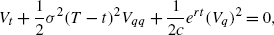
  with boundary condition

  

  and the allowance price is given by

  

• (b) Assuming that the emission rate before abatement activities is given by the White–Noise process in Lemma 6.27. Then the characteristic PDE of the allowance price is given by

  

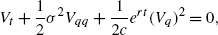
  and there is an analytical formula for the allowance price:

  

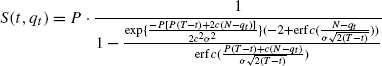
  where $\operatorname{erf}c(x)=1-\operatorname{erf}(x)=\frac{2}{\sqrt{\pi}}\int^{\infty}_{x} e^{-t^{2}}\,dt$ is the complementary error function.

Proof 13 (Idea)

Similar to the proof of Lemma 6.13, Itô’s lemma and Lemma 6.27 imply

By the principle of optimality

(A.21)

Subtracting V(t,q _t ) on both sides of Eq. (A.21) yields

(A.22)

Maximizing the expression within the curly brackets by deriving it with respect to α _t and setting it to zero yields

(A.23)

The characteristic PDE is obtained by setting the expression within the curly brackets in Eq. (A.22) to zero and by inserting the formula for α _t into this equation:

(A.24)

The spot price equals marginal abatement costs as shown in Lemma 6.13, that is,

• (a) The proof is completed by using (ii) of Lemma 6.27.

• (b) The characteristic PDE follows directly from Eq. (A.24) by using part (i) of Lemma 6.27. A solution of this PDE is derived by Seifert et al. (2008). □

References

Alberola, E., & Chevallier, J. (2009). European carbon prices and banking restrictions: evidence from phase I. Energy Journal, 30, 51–80.
Barro, R., & Sala-i Martin, X. (1995). Economic growth. New York: McGraw-Hill.
Benz, E., & Trück, S. (2008). Modeling the price dynamics of CO2 emission allowances. Energy Economics, 31(1), 4–15.
Brigo, D., Dalessandro, A., Neugebauer, M., & Triki, F. (2009). A stochastic processes toolkit for risk management: geometric Brownian motion, jumps, GARCH and variance gamma models. Journal of Risk Management in Financial Institutions, 2(4), 365–393.
Bunn, D., & Fezzi, C. (2009). Structural interactions of European carbon trading and energy prices. The Journal of Energy Markets, 4, 53–69.
Carmona, R., Fehr, M., Hinz, J., & Porchet, A. (2009). Market design for emission trading schemes. SIAM Review, 9(3), 465–469.
Chesney, M., & Taschini, L. (2012). The endogenous price dynamics of emission allowances and an application to CO2 option pricing. Applied Mathematical Finance, 19(5), 447–475.
Chevallier, J. (2011). Econometric analysis of carbon markets: the European union emission trading scheme and the clean development mechanism. Berlin: Springer.
Cleveland, R. B., Cleveland, W. S., McRae, J., & Terpenning, I. (1990). STL: a seasonal-trend decomposition procedure based on loess. Journal of Official Statistics, 6(1), 3–73.
Creti, A., Jouvet, P., & Mignon, V. (2012). Carbon price drivers: phase I versus phase II equilibrium? Energy Economics, 34(1), 327–334.
Crocker, T. (1966). The economics of air pollution: Vol. 1. The structuring of atmospheric pollution control systems. New York: Harold Wolozin.
Cronshaw, M. B., & Kruse, J. B. (1996). Regulated firms in pollution permit markets with banking. Journal of Regulatory Economics, 9, 179–189.
Dales, J. (1968). Pollution property and prices. Toronto: University of Toronto Press.
Daskalakis, G., Psychoyios, D., & Markellos, R. N. (2009). Modeling CO2 emission allowance prices and derivatives: evidence from the European trading scheme. Journal of Banking & Finance, 33(7), 1230–1241.
Fusai, G., & Roncoroni, A. (2008). Implementing models in quantitative finance: methods and cases. Berlin: Springer.
Gronwald, M., Ketterer, J., & Trück, S. (2011). The dependence structure between carbon emission allowances and financial markets—a copula analysis. Economic Record, 87(1), 105–124.
Grüll, G., & Kiesel, R. (2009). Pricing CO 2 permits using approximation approaches. Preprint.
Hintermann, B. (2010). Allowance price drivers in the first phase of the EU ETS. Journal of Environmental Economics and Managements, 59(1), 43–56.
Kijima, M., Maeda, A., & Nishide, K. (2010). Equilibrium pricing of contingent claims in tradable permit markets. The Journal of Futures Markets, 30(6), 559–589.
Kling, C., & Rubin, J. D. (1997). Bankable permits for the control of environmental pollution. Journal of Public Economics, 64, 101–115.
Montgomery, W. (1972b). Markets in licenses and efficient pollution control programs. Journal of Economic Theory, 5, 395–418.
Paolella, M. S., & Taschini, L. (2008). An econometric analysis of emission–allowances prices. Journal of Banking & Finance, 32(10), 2022–2032.
Pontryagin, L., Boltayanskii, V., Gamkrelidze, R., & Mishchenko, E. (1962). The mathematical theory of optimal processes. New York: Wiley.
Rubin, J. D. (1996). A model of intertemporal emission trading, banking, and borrowing. Journal of Environmental Economics and Management, 31, 269–286.
Seifert, J., Uhrig-Homburg, M., & Wagner, M. (2008). Dynamic behavior of CO2 spot prices. Journal of Environmental Economics and Managements, 56, 180–194.
Taschini, L., & Urech, S. (2010). The real option to fuel switch in the presence of expected windfall profits under the EU ETS. Journal of Energy Markets, 3(2), 27–47.
Tietenberg, T. (1985). Emission trading: an exercise in reforming pollution policy. Working paper, Resources for the Future, Washington D.C.
Uhrig-Homburg, M., & Wagner, M. (2007). Futures price dynamics of CO 2 emission certificates—an empirical analysis. Preprint.
Author information
Authors and Affiliations