
Abstract
At the Cambridge Astronomical Survey Unit (CASU) we are responsible for the development and implementation of a number of pipelines for the routine processing of large area near-infrared surveys. In this paper, we discuss some of the challenges we face when tackling the large volumes of data generated nightly from WFCAM on UKIRT and VIRCAM on VISTA.
Keywords
These keywords were added by machine and not by the authors. This process is experimental and the keywords may be updated as the learning algorithm improves.
1 Introduction
VISTA Footnote 1alone requires 3 distinct pipelines, run in 3 different places:
-
1.
Paranal pipeline: data from VISTA are assessed for quality control (QC) in real time at the summit using a simplified data reduction pipeline. Because these reductions have to happen very rapidly and in a causal sequence, this pipeline relies on previously prepared library calibration information.
-
2.
Garching pipeline: the raw data are then collected onto USB discs, which are shipped to Garching and ingested into the ESO raw data archive. A second pipeline is run, used to monitor instrumental health, generate calibration information and to provide library calibration frames for the summit pipeline. More up-to-date calibration information is applied and the quality control results are correspondingly better.
-
3.
Cambridge pipeline: once the archive ingestion is done, the same USB discs are forwarded to Cambridge for science data processing. When running the science pipeline we are able to consider an entire night of data (or indeed a whole week of data) as a single entity and hence we can use information which is not available to the ESO pipelines. This leads to a much better result than can be obtained with the QC pipelines.
The Cambridge pipeline products (astrometrically and photometrically calibrated images and catalogues) can then be accessed by the survey participants either directly from Cambridge, or via the VISTA and WFCAM Science Archives (VSA, WSA) both hosted at the Royal Observatory in Edinburgh.
2 Processing of VIRCAM and WFCAM Images
Observing in the near infrared is a little like observing in the daytime, the vast majority of interesting sources are much fainter than the bright and variable night-time sky. Modern infrared detectors are now very sensitive, but they do tend to suffer from significant instrumental features. The most pernicious of these are described below, together with a short outline of how they are removed.
-
Reset correction: this is similar but not the same as a debias operation in CCD processing. Reset frames are taken for each exposure and are subtracted in the data acquisition system. Although this is not a pipeline reduction step per se, it is important to realise that this happens as it has an impact when estimating the linearity of the detectors.
-
Dark correction: the dark current is estimated from a series of exposures taken with a dark filter inserted. Subtracting a mean dark frame also corrects several other additive electronic effects, such as residual reset correction anomalies.
-
Linearity correction: although the WFCAM detectors are linear, the VIRCAM detectors do not have a linear response. To estimate the non-linearity of each detector we need information on the readout timing, the exposure time and the reset image timing (this is because there is no shutter on the camera and in double-correlated sampling mode, the default, the reset frame is subtracted prior to writing images to disk).
-
Flat field correction: dividing by a mean twilight flatfield image removes the small scale QE variations in the detector as well as the large scale vignetting profile of the camera. We also use the global flatfield properties of each detector to gain-normalise each detector to a common (median) system.
-
Sky background correction: this removes the large scale spatial background emission that comes from the atmosphere as well as several remaining additive effects. The 2-D background map is estimated using several different algorithms that combine the science images themselves with rejection or masking. Sometimes when large extended objects are present it is necessary to use offset sky exposures to get a background map. Automating this correctly is one of the most difficult parts of near-infrared image processing. Figure 1 shows an example of a WFCAM image with and without sky subtraction.
Fig. 1 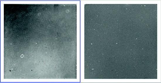
Images from WFCAM with and without the skysubtraction applied
-
Destripe: the readout electronics for the VIRCAM detectors introduce a low-level horizontal stripe pattern into the background. Every exposure yields a different pattern, but groups of four detectors, readout through the same IRACE controllers, have the same pattern on a given exposure. This means there a great deal of redundancy when it comes to estimating the stripe pattern. WFCAM shows a similar pattern, but with a different symmetry due to the detector properties.
-
Jitter stacking: infrared detectors often have large numbers of cosmetic defects implying infrared imaging is invariably done in a jitter mode, whereby an observation of a region is broken up into several shorter exposures and the telescope moved slightly between them. At this point in the reduction the jitter series is shifted and combined to form a single image stack, using positions of detected objects on all the detectors to compute the shifts. This allows bad pixel regions in one exposure to be rejected in favour of good pixels in other exposures.

Two corrections not discussed above and not implemented for either VIRCAM and WFCAM are: a fringe correction which is at a very low level for both instruments and is automatically dealt with during sky subtraction, and a crosstalk correction which is very significant in WFCAM (and very hard to remove without compromising the images), and not seen with VIRCAM. We also looked for evidence of persistence, which manifests itself as a glow on a detector where a bright object was recently observed. For both the WFCAM and VIRCAM detectors this turned out to be a very small and unpredictable effect which only occurred when extremely bright stars (which are rare) are observed. In practice this effect is negligible and is therefore ignored during pipeline processing.
3 Astrometric Calibration
The astrometric solution for each image taken with VIRCAM or WFCAM is derived from 2MASS. The WCS distortion model used for both instruments is based on the ZPN projection. For a purely radial distortion, this relates the true on-sky radial distance from the optical axis to the measured radial distance in the focal plane in the form:
where k1 is the plate scale at the centre, and k3, k5 etc describe the distortion relative to the angular distance on the focal plane. For WFCAM, k5 is negligable. For VIRCAM k1 = 0. 3413 arcsec/pixel (i.e. 17.065 arcsec/mm) and in angular units the distortion coefficients are given quite accurately by \(k3/k1 = 44\) and \(k5/k1 = -\)10300 (using angular measures in radians). Higher order terms are negligible. After distortion correction the residuals from individual detector linear fits can be used to monitor the quality of the 2MASS-based astrometric solution which has a rms of around 80 milliarcseconds for both WFCAM and VIRCAM, dominated by the 2MASS errors (see Fig. 2).

The cumulative density function of VIRCAM WCS rms values on each filter for all chips, using seven nights of science verification data from Oct 2009. For each filter the number of chips used, median and 10 and 90% quantiles are shown
4 Photometric Calibration
The photometric calibration, like the astrometric calibration, is derived from 2MASS, following the methods outlined in [2]. The unsaturated 2MASS stars that are observed in every VIRCAM/WFCAM exposure can be used to derive a single photometric zeropoint for every image (after correcting the 2MASS photometry into the appropriate observing filter system, see Fig. 3).

Hess diagrams to show the measurements of VISTA-2MASS colours for data taken on clear nights in regions of low reddening. The blue lines show the colour equations currently in use
Stacking 2MASS zeropoints over long timescales allows us to measure residual spatially-dependent illumination corrections in the data and, for WFCAM, to reach accuracies of 2% in ZY and 1.5% for the JHK bands. With VIRCAM, the illumination corrections look significantly smaller, and we are currently quanitfying the accuracy of the calibration. Obvious benefits of this strategy include a reduction in the observing time required to monitor photometric standards, and the ability to recover the calibration for data taken through thin cirrus. A caveat is that the photometric calibration becomes less robust for regions of extremely high reddening, though this is a relatively small fraction of the sky.
In addition to astrometric effects the change in scale as a function of radius also creates photometric complications. The aim of conventional flatfielding is to create a flat background by normalising out perceived variations from uniformly illuminated frames. If the sky area per pixel changes then this is reflected in a systematic error in the derived photometry. However, since it is much simpler to deal with “flat” backgrounds, this problem is either usually ignored or corrected during later processing stages, together with other systematic photometry effects. The amount of photometric distortion amounts to a 3.5% effect at the edge of the field for VIRCAM, and 1.2–1.7% (wavelength-dependent) for WFCAM.
5 From Pawprints to Tiles
A standard VIRCAM tile image is made up from 6 stacked pawprints each containing 16 detector-level images. The sky level on all 96 component images is adjusted to the same level and the components are then projected (drizzled) onto a single Tangent Plane WCS image. During the projection the pixel intensities with respect to sky are adjusted to account for the spatially-dependent photometric distortion within the original ZPN pawprints. Thus no additional photometric distortion correction is necessary for tiled products with VIRCAM (This is not the case for WFCAM where the final products are pawprint based, because the overlaps are not required to achieve full survey depth). Creating tiled images in this simple way has the advantange of preserving edge structures and other artefacts to aid in visual inspection of, say, candidate rare objects and enables most large scale structures to be retained for further investigation (Fig. 4).

VIRCAM comprises 16 2k ×2k Ratheon detectors, each with a Field of view of 11. 6 ×11. 6 arcmin. 6 pointings are required for continuous uniform coverage. A single pointing is called a pawprint (it made sense when we had 4 array devices with WFCAM), and 6 make a tile with a combined field of view of 1 ×1.5 deg
The drawback from a catalogue generating point of view is that edges between detectors can often introduce spurious structures and also subsequent spurious objects in the catalogues. For more reliable catalogue generation from tiles we pre-filter each stacked pawprint image using a nebulosity filter (see below) to remove all structure on scales of 30 arcsec and over. This filter is also fairly adept at reducing edge effects between pawprints. These filtered images are tiled in exactly the same way as previously but since the background is guaranteed to be completely flat for each detector image, the resulting tile image is much more uniform, since it is by design devoid of any large-scale background structure. The tile catalogues are then created from these images (Fig. 4).
Each detector potentially has a different PSF and together with the varying seeing conditions that can happen during the observation of a tile this means that there are normally 96 different PSFs which contribute to a single tile (some of which are combined in the overlap areas). In order to compute the corrections for the aperture fluxes we assume that the PSF does not vary across the tile. This will inevitably introduce spatial photometric distortions at the level of at least 1–2% over the tile, and we are currently investigating ways of correcting this for VISTA tiles (Fig. 5).

The image shows the systematics in photometry arising from a standard VISTA 6 pointing tile. The systematics vary from 0% in the centre (dark) up to 3% toward the corners (light)
6 The Nebuliser
Traditional methods for source detection first model the background with a single-pass smoothly varying map. Sources are then detected as significant connected pixels above the local background estimate (see e.g. [3, 1]). This works well for most of the sky, however in regions of bright, spatially-varying nebulosity, traditional background following is insufficient, even after increasing the resolution of the background map. An example of such a region is illustrated in Fig. 6, which shows WFCAM K-band observations of M17, taken as part of the UKIDSS Galactic Plane Survey. To handle such data we are using a new aproach, nicknamed the Nebuliser [4]. The Nebuliser works by constructing a non-linear iteratively smoothed version of the image, which attempts to decouple objects from background on the basis of their spatial frequency and hence generate a usable background map. The results of running the algorithm on the M17 data are shown in Fig. 6

Spatially splitting the WFCAM image of M17 (left) into small-scale features (the stars, centre) and large-scale features (the background and nebulosity, right) using iteratively clipped non-linear filtering
The algorithm is also extremely useful in the construction of tiles (see above). The code for this algorithm is now available to the community in the CASUTools package, which can be obtained from our website.Footnote 2 For more information and additional support, please contact us via email.Footnote 3
Notes
- 1.
- 2.
- 3.
email:casuhelp@ast.cam.ac.uk.
References
Bertin, E., Arnouts, S.: Astron. Astrophys. Suppl. 117, 393 (1996)
Hodgkin, S.T., Irwin, M.J., Hewett, P.C., Warren, S.J.: Mon. Not. R. Astron. Soc. 394, 675 (2009)
Irwin, M.J.: Mon. Not. R. Astron. Soc. 214, 575 (1985)
Irwin, M.J.: UKIRT Newsl. 26, 14 (2010)
Author information
Authors and Affiliations
Corresponding author
Editor information
Editors and Affiliations
Rights and permissions
Copyright information
© 2012 Springer-Verlag Berlin Heidelberg
About this paper
Cite this paper
Hodgkin, S., Irwin, M., Lewis, J., Gonzalez-Solares, E., Yoldaş, A.K. (2012). Processing Data from Large Infrared Surveys. In: Moitinho, A., Alves, J. (eds) Star Clusters in the Era of Large Surveys. Astrophysics and Space Science Proceedings. Springer, Berlin, Heidelberg. https://doi.org/10.1007/978-3-642-22113-2_5
Download citation
DOI: https://doi.org/10.1007/978-3-642-22113-2_5
Published:
Publisher Name: Springer, Berlin, Heidelberg
Print ISBN: 978-3-642-22112-5
Online ISBN: 978-3-642-22113-2
eBook Packages: Physics and AstronomyPhysics and Astronomy (R0)