A Cost-Effective Data Replica Placement Strategy Based on Hybrid Genetic Algorithm for Cloud Services

Abstract

Cloud computing provide an efficient big data processing platform for many small and medium scale enterprises, how to replicate and allocate data in clouds is a critical problem influencing cost consumption for small and medium scale enterprises. Cloud data management systems mainly serve two kinds of workloads, one is read-intensive analytical workloads (e.g. OLAP), the other is write-intensive transactional workloads (e.g. OLTP). It is essential to minimize data management costs like storage, communication bandwidth, update and power with guaranteeing the service level agreements. Toward two workloads, a cost-effective data replica placement approach for minimizing data management costs on cloud computing centers is proposed. The definition of different data management costs is identified first, then we construct the cost optimization model of the data replica placement problem. The paper proposes a hybrid genetic algorithm and a data support-based initialization method that addresses the problem. Experiments show that the approach result in significant reduction in total data management cost and the algorithm is with good performance.

1 Introduction

With the development and popularization of internet technique, a wealth of data is generated in commercial applications, such as e-commerce, web search, social media, online map and so on. One billion pictures are uploaded to Facebook every week, which means that nearly 60 TB new data will be generated per week, the amount of traffic flowing over the internet annually exceeds 700 EB, more than one million transactions are processed per hour in Wal-Mart, the volume of data will reach 25 PB [10, 11]. Cloud computing technology [2] integrates hardware and software resources among data centers through the Internet, which provides small and medium scale enterprises with a reliable platform for storing, processing, and analyzing big data. In order to improve the performance of applications and the reliability of user access, data replication technology is widely used in cloud platforms [19]. For example, YouTube deploys copies of video in different geographic locations to provide users with video copies in nearby clouds, this technology significantly shortens the request response time for users, and greatly improves user experience and service quality, meanwhile, due to the presence of redundant information, it also guarantees the reliability of the service.

Neves et al. [13] proposed a data replication technology in content distribution networks. The article replicates the data to a subset of entire servers for responding users’ requests, and aims to minimize the data traffic cost in the network. Bektas et al. [3] presented an integer non-linear programming model, which jointly determines the number and location of servers, data replica allocation to servers, and query routing problems. The model minimizes the total server placement and data transmission costs. Yuan et al. [18] developed a practical storage strategy that can automatically decide whether to store the generated data set in clouds. This strategy firstly focuses on the tradeoff between data calculation and storage cost, then considers the user’s storage option preference. Nehme et al. [12] proposed an approach that automatically partitions the database according to the expected workload. The method tightly integrates the query optimizer that relies on database statistics, and emphatically considers read-intensive analytical workloads. Curino et al. [5] adopted a graph-based partitioning algorithm to minimize the number of distributed transactions for OLTP workloads. However, this method eliminates fault tolerance by not replicating data items with high-frequency write/update operations. Tatarowicz et al. [15] utilized a router with high memory and powerful computing resources for data search, but this method isn’t cost-effective on account of occupying a large amount of memory and computing resources. Johansson et al. [9], Ferhatosmanoǧlu et al. [7] and Tosun et al. [16, 17] proposed a comprehensive combination of data replication allocation and query processing strategies to minimize latency and query response time. Nevertheless, the method ignores cost consumption and the impact of data updates generated by write-intensive transactional workloads (OLTP) on the transmission.

Therefore, in this paper, from the view of data management costs, a genetic algorithm-based heuristic method oriented to two types of workloads (read-intensive analytical workload and write-intensive transactional workload) is developed to synthetically consider data storage, update, transmission and processing costs in clouds. The method aims to minimize total data management costs, and jointly determines the number of servers in the cloud storage system, the number of data replicas, the storage location of data replicas, and user access paths to data replicas. Experiments confirm that the method reduces data management costs in clouds and the proposed algorithm performs well.

We organize the rest of this paper as follows. Section 2 provides the problem definition and formulation. Section 3 introduces the procedure of the genetic algorithm-based heuristic developed to solve the problem. Section 4 presents the extensive experiments designed to evaluate the effectiveness and efficiency of the proposed algorithm. Section 5 concludes the contribution of this work.

2 Problem Statement

2.1 Cloud Computing Environment

Figure 1 illustrates the cloud computing environment, data center, user, network and site server constitutes the heart of a cloud service. Data centers distributed in different geographical that are interconnected through communication links constitute the main environment of cloud computing. The data is transmitted over the network to the data center closest to the user for satisfying various requirements. Servers handle data computing and storage.

Fig. 1.

Example of the cloud computing environment

Figure 2 shows an illustrative example that vividly demonstrates the impact of data replication and placement on data management costs in clouds. There are 2 user queries, 4 data centers (1 server in each data center), 8 data items and 2 different data layouts in the cloud service. Query $q_{1}$ accesses data items $d_{1} ,d_{2} ,d_{4} ,d_{5}$, query $q_{2}$ accesses data items $d_{3} ,d_{7} ,d_{8}$. For simplicity, we assume that the server’s computing power, data storage cost and calculation cost are the same, 8 data items are all 3 GB, and the transmission cost among data centers are the same. Taking Amazon Elastic Compute Cloud as an example [1], data management costs are shown in Table 1. Therefore, the data management cost generated by Alternative I is: 0.19/GB * 6 GB (data transmission cost) + 0.19/GB * 3 GB (data transmission cost) + 0.11/GB * 24 GB (data storage cost) = $4.11; the total cost generated by Alternative II is: 0.19/GB * 6 GB (data transmission cost) + 0 (data transmission cost) + 0.11/GB * 27 GB (data storage cost) = $3.84. Obviously, the data replication and placement strategy greatly influences data management costs in clouds.

Fig. 2.

A data placement example in clouds

Table 1. Cloud service costs in Amazon elastic compute cloud

2.2 Data Management Cost Model in Clouds

With given data items set $K = \left\{ {k:k = 1,2, \ldots ,p} \right\}$, server nodes set $J = \left\{ {j:j = 1,2, \ldots ,m} \right\}$, user nodes set $I = \left\{ {i:i = 1,2, \ldots ,n} \right\}$, the data management cost problem in clouds is defined as follows:

Definition 1.

Server installation cost: It is assumed that data processing and storage occurs on the server. The server is the basis for providing users with various cloud services, and its installation cost is an important part of data management costs. $F_{\begin{subarray}{l} j \\ \end{subarray} }$ denotes the fixed cost to install a sever at location j.

Definition 2.

Data placement cost: The unit storage and maintenance cost of data item k that occurs on a server at location j is $\Omega _{j}$, the size of data item k is $s_{k}$, then, the total storage and maintenance cost is $\Omega _{j} * s_{k}$. When a write-intensive transactional workload occurs, the amount of user update requests at node i for data items k during the unit communication time is $u_{ik}$, the unit transmission cost that occurs on the path where user at node i accesses data item k at location j is $t_{ij}$. Thus, the data placement cost of data item k replica occurs on the server at location j is $P_{jk} =\Omega _{j} * s_{k} + \sum\nolimits_{i = 1}^{n} {u_{ik} * t_{ij} }$.

Definition 3.

Data transmission cost: When a read-intensive analytical workload occurs, the query frequency of the user at location i accessing data item k is $f_{ik}$, The unit transmission cost occurred on the path where the user at node i accessing the data item k at server j is $b_{ij}$ Therefore, the transmission cost required for executing user node i’s query over data item k at location j is: $T_{ijk} = f_{ik} *b_{ij} *s_{k}$.

2.3 Data Management Cost Optimization Model in Clouds

A mathematical programming model for the data management cost optimization in clouds is presented. The problem objective is to jointly determine

• (1) the number of servers in the cloud storage system,

• (2) the number of data replicas,

• (3) the storage location of data replicas, and

• (4) user access paths to data replicas.

Decision variables are as follows:

$$ Z_{j} = \left\{ {\begin{array}{*{20}l} {1,} \hfill & {{\text{if}}\;{\text{a}}\;{\text{server}}\;{\text{is}}\;{\text{installed}}\;{\text{at}}\;{\text{location}}\;{\text{j}}} \hfill \\ {0,} \hfill & {\text{otherwise}} \hfill \\ \end{array} } \right. $$

$$ {\text{y}}_{\text{jk}} = \left\{ {\begin{array}{*{20}l} { 1 ,} \hfill & {{\text{if}}\;{\text{a}}\;{\text{replica}}\;{\text{of}}\;{\text{data}}\;{\text{item}}\;{\text{k}}\;{\text{is}}\;{\text{allocated}}\;{\text{to}}\;{\text{a}}\;{\text{server}}\;{\text{at}}\;{\text{location}}\;{\text{j}}} \hfill \\ { 0 ,} \hfill & {\text{otherwise}} \hfill \\ \end{array} } \right. $$

$$ {\text{x}}_{\text{ijk}} { = }\left\{ {\begin{array}{*{20}l} 1, \hfill & {{\text{if}}\;{\text{user}}\;{\text{node}}\;{\text{i's}}\;{\text{query}}\;{\text{request}}\;{\text{to}}\;{\text{data}}\;{\text{item}}\;{\text{k}}\;{\text{is}}\;{\text{served}}\;{\text{from}}\;{\text{a}}\;{\text{server}}\;{\text{at}}\;{\text{location}}\;{\text{j}}} \hfill \\ 0, \hfill & {\text{otherwise}} \hfill \\ \end{array} } \right. $$

The data management cost optimization in clouds problem is formulated as:

$$ \hbox{min} \sum\limits_{j = 1}^{m} {F_{j} *z_{j} + \sum\limits_{j = 1}^{m} {\sum\limits_{k = 1}^{p} {P_{jk} *y_{jk} + \sum\limits_{i = 1}^{n} {\sum\limits_{j = 1}^{m} {\sum\limits_{k = 1}^{p} {T_{ijk} *x_{ijk} } } } } } } $$

(1)

s.t.

$$ \sum\limits_{j = 1}^{m} {\sum\limits_{k = 1}^{p} {a_{ik} *x_{ijk} = b_{i} ,\;\forall i \in I} } $$

(2)

$$ x_{ijk} \le y_{jk} ,\;\forall i \in I,\;j \in J,\;k \in K $$

(3)

$$ y_{jk} \le z_{j} ,\;\forall j \in J,\;k \in K $$

(4)

$$ \sum\limits_{j = 1}^{m} {y_{jk} \ge N_{\hbox{min} } ,\;\forall k \in K} $$

(5)

$$ \sum\limits_{k = 1}^{p} {s_{k} * y_{jk} \le S_{j} * z_{j} ,\forall j \in J} $$

(6)

According to Sect. 2.2, the first term in the objective function (1) represents the fixed costs for installing servers, the second term presents storage costs, maintenance costs and update costs associated with data placed in servers, and the third term is the data transmission cost associated with responding user queries.

Constraint (2) guarantees that the demand for queries to data items by each user is satisfied. $A = \left[ {\begin{array}{*{20}c} {a_{11} } & \cdots & {a_{1k} } & \cdots & {a_{1p} } \\ \vdots & {} & \vdots & {} & \vdots \\ {a_{i1} } & \cdots & {a_{ik} } & \cdots & {a_{ip} } \\ \vdots & {} & \vdots & {} & \vdots \\ {a_{m1} } & \cdots & {a_{mk} } & \cdots & {a_{mp} } \\ \end{array} } \right]\left[ {\begin{array}{*{20}c} {b_{1} } \\ \vdots \\ {b_{i} } \\ \vdots \\ {b_{m} } \\ \end{array} } \right]$ denotes users accessing data query matrix, $a_{ik} = 1$ denotes that user node i has a request for the data item k, $b_{i}$ denotes the number of data accessed by users. The query matrix shown in Fig. 2 is $A = \left[ {\begin{array}{*{20}c} 1 & 1 & 0 & 1 & 1 & 0 & 0 & 0 \\ 0 & 0 & 1 & 0 & 0 & 0 & 1 & 1 \\ \end{array} } \right]\left[ {\begin{array}{*{20}c} 4 \\ 3 \\ \end{array} } \right]$.

Constraint (3) ensures that a user node accesses a server which has been installed at the corresponding location.

Constraint (4) prevents the assignment of a data replica to a server unless the server is installed.

Constraint (5) specifies the minimum number of replicas of data items to guarantee the security and reliability of cloud services.

Constraint (6) dictates that the size of the data items stored in a server cannot exceed the storage capacity of the server. The storage capacity of the server j is $S_{j}$.

3 Solution Procedure

The problem of data replica placement in clouds is a complex combinational optimization problem. More and more scholars utilize the genetic algorithm combined with heuristic rules to solve combinatorial optimization problems, and these methods achieved good results. This paper proposes a hybrid genetic algorithm (hereafter called HGA) to solve the problem and designs a heuristic rule based on the data support degree to form initial population for accelerating algorithm optimization. We also apply this rule to genetic operators to enhance the effectiveness of local search.

3.1 Chromosome Design

Because the objective function of the research problem in this paper depends not only on the choice of server, but also on the data replication and placement on the server, so this paper adopts a group-based chromosome representation method proposed by Falkenauer [6]. This encoding consists of two parts, the part below shows the servers where the data is stored and the upper represents the data replica placed on the server. Figure 3 shows an example of encoding according to Fig. 2.

Fig. 3.

An example of chromosome representation

In Fig. 3, a letter represents a server, a numeral denotes a data replica. The upper data layout shows that data replica 1, 5 are placed on server A, data replica 2, 6 are placed on server B, data replica 3, 7 are placed on server C, data replica 4, 8 are placed on server D.

3.2 Initial Population Generation

Definition 4.

Data support degree: the percentage of the number of queries supported by data i that accounts for the total number of queries supported by each data.

As shown in Fig. 2, the four queries are $q_{1} \left\{ {d_{1} ,d_{2} ,d_{4} ,d_{5} } \right\}$, $q_{2} \left\{ {d_{3} ,d_{7} ,d_{8} } \right\}$, $q_{3} \left\{ {d_{1} ,d_{3} } \right\}$ and $q_{4} \left\{ {d_{2} ,d_{4} ,d_{6} } \right\}$ respectively, the number of queries supported by each data are $d_{1} \left\langle {q_{1} ,q_{3} } \right\rangle = 2$, $d_{2} \left\langle {q_{1} ,q_{4} } \right\rangle = 2$, $d_{3} \left\langle {q_{2} ,q_{3} } \right\rangle = 2$, $d_{4} \left\langle {q_{1} ,q_{4} } \right\rangle = 2$, $d_{5} \left\langle {q_{1} } \right\rangle = 1$, $d_{6} \left\langle {q_{4} } \right\rangle = 1$, $d_{7} \left\langle {q_{2} } \right\rangle = 1$ and $d_{8} \left\langle {q_{2} } \right\rangle = 1$. Thus, the support degree of data $d_{1}$, $s(d_{1} )$, equals $\frac{2}{12}$, the rest data support degree can be calculated in the same manner.

The number of data replicas according to data support degree is computed before generating the initial population, the number of data k’s replicas is computed as $N_{k} = [\frac{{s\left( {d_{k} } \right) \,*\, \sum\limits_{j = 1}^{m} {S_{j} } }}{{s_{k} }}]$, [] represents rounding. Generating pop initial individuals with various number of servers. The data is sorted in descending order according to the data support degree, and the data replica is placed on the server nearest to the query node. The procedure of the initial Population Generation algorithm based on data Support degree (PGoS) is as follows:

• (1) The data items are sorted in descending order according to the data support degree. The servers that correspond to each data item in the individual are sorted in ascending order according to the distance between the server node and the query node the data can support. The data item is placed in descending order according to the data support degree. The current data item is placed on the first corresponding server. If the storage capacity of the first server is insufficient, the data item is placed on the second corresponding server, and so on. If all the servers’ storage capacity is insufficient, new servers will be selected from the unselected server set for data placement until all data items (which do not contain a replica of the data at this time) are placed on the server. This step guarantees that constraints (2), (4) and (6) are satisfied, which effectively avoids infeasible solutions.

• (2) The data replicas are placed on servers in turn according to descending order of the data support degree. The first replica of the first data item is placed on the second corresponding server. If the second corresponding server is insufficient, then the first replica of the first data item is placed on the third corresponding server, and so on, until all $N_{k} - 1$ replicas are placed on servers or all servers have been inspected for storage capacity.

• (3) Checking whether the placed replicas satisfy constraint (6). If all replicas of the first data item can be placed, then moving on to step (2) for placing replicas of the next data item; if only a partial replica of the first data item are placed after all servers’ storage capacity has been checked, then deleting the remaining replicas and going to step (2) for placing replicas of the next data item, and so on.

• (4) If all servers’ storage capacity is satisfied and no replicas can be placed, the placement of replicas are completed, then deleting the remaining replicas. The termination of the PGoS algorithm. The algorithm flowchart is presented in Fig. 4.

  Fig. 4.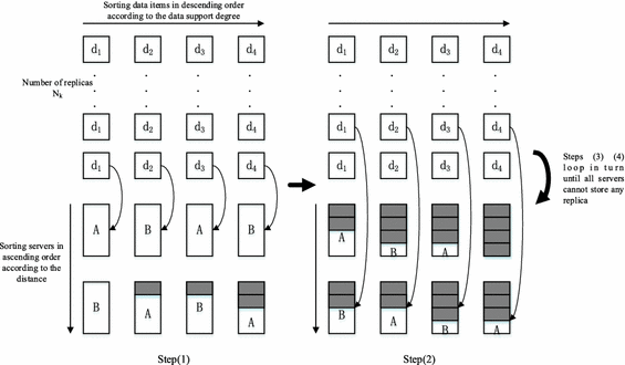

  

  The flow diagram of PGoS algorithm

3.3 Fitness Function

The encoding of each chromosome directly determines the value of the decision variable $y_{jk} ,z_{j}$. The original model is simplified as:

$$ \hbox{min} \sum\limits_{j = 1}^{m} {F_{j} *\overline{{z_{j} }} + \sum\limits_{j = 1}^{m} {\sum\limits_{k = 1}^{p} {P_{jk} *\overline{{y_{jl} }} + \sum\limits_{i = 1}^{n} {\sum\limits_{j = 1}^{m} {\sum\limits_{k = 1}^{p} {T_{ijk} *x_{ijk} } } } } } } $$

(7)

s.t.

$$ \sum\limits_{j = 1}^{m} {\sum\limits_{k = 1}^{p} {a_{ik} *x_{ijk} = b_{i} ,\;\forall i \in I} } $$

(8)

$$ x_{ijk} \le \overline{{y_{jk} }} ,\;\forall i \in I,\;j \in J,\;k \in K $$

(9)

$$ x_{ijk} \in \left\{ {0,1} \right\} $$

(10)

The simplified model is a classical user assignment problem (UAP) model, and Sen et al. [14] reviews various methods to quickly and efficiently solve the UAP problem. Because this paper deals with the cost minimization problem, it is necessary to convert the objective function into a fitness function to ensure that excellent individuals have large fitness values. For an individual $v_{i}$, the fitness function is:

$$ F\left( {v_{i} } \right) = \frac{{f_{\hbox{max} } - f(v_{i} )}}{{f_{\hbox{max} } - f_{\hbox{min} } }} $$

$f_{\hbox{max} }$ is the value corresponding to the worst individual in the current population, $f_{\hbox{min} }$ is the value corresponding to the best individual in the current population, so the fitness value can reflect the distance of each individual in the population from the worst individual.

3.4 Genetic Operators

Selection Operator

This paper adopts the elitism selection combined with the roulette wheel selection for selecting individuals.

• (1) Calculating the individual fitness value according to the above mentioned strategy. Individuals with the highest fitness value are selected into the next generation.

• (2) Calculating the probability that each individual enters into the next generation according to its fitness value:

  $$ p\left( {v_{i} } \right) = \frac{{F\left( {v_{i} } \right)}}{{\sum {F\left( {v_{i} } \right)} }} $$

Crossover Operator

According to the encoding method described in Sect. 3.1, the crossover operator requires processing chromosomes of variable length. The specific crossover process is illustrated in Fig. 5.

• (1) Selecting two parent individuals with probability $p_{c}$. Selecting two crossover point randomly, and selecting the crossover portion of each parent.

• (2) Inserting the crossover part of the first parent in front of the crossover point of the second parent and inserting the crossover part of the second parent in front of the crossover point of the first parent.

• (3) If the newly inserted server already exists on the parent chromosome, the original server is deleted. The data replicas in the original server that exists in the new server is directly deleted, and replicas that do not exist in the new server are rearranged using algorithm PGoS.

• (4) If the newly inserted server does not exist in the parent chromosome, taking out the same replicas placed in the new server and the other servers, then taken out replicas will be rearranged by using algorithm PGoS.

Fig. 5.

The crossover operator sketch

Mutation Operator

The mutation operator is difficult to perform effective local search in genetic algorithm at later process. Therefore, this paper also embeds the neighborhood search mechanism based on data support degree into the mutation operator to improve the search efficiency and evolution quality. The probability of mutation is set as $p_{m}$. $pop*p_{m}$ individuals are selected from the population for mutation. Randomly generating binary number $\left[ {0,1} \right]$, if it is 1, enabling a new server; if it is 0, deleting a deployed server. The mutated individuals that lack partial data will be rearranged by using algorithm PGoS.

4 Experiment

The experiment was performed in the MATLAB environment. The computer was configured with an Intel Core i3-4150 CPU and RAM 4.00 GB. The relevant data management cost parameters in clouds involved in the experiment: server installation cost, data storage cost, and transmission cost are all obtained through Amazon’s EC2 [8]. Data items and related user information are obtained through the Dataset for “Statistics and Social Network of YouTube Videos”. The distance between data centers is obtained through GPSSPG.

4.1 The Validity of the Proposed Algorithm

In order to verify the quality of the proposed algorithm (HGA), this paper uses CPLEX [4] to solve the optimal solution of the integer programming (IP) model built in this paper, and uses the genetic algorithm (GA) as a comparison. The instances scale and algorithm parameter settings are shown in Tables 2 and 3, respectively. Experimental results are shown in Table 4.

Table 2. Instances scale

Table 3. Parameters of HGA and GA

Table 4. Experimental results

Experimental results demonstrate that the quality of the solution obtained by HGA is very close to the optimal solution, and the distance between the solution obtained by HGA and the optimal solution can be controlled at around 1.22%, which is obviously better than the simple genetic algorithm. It shows that the heuristic rule based on data support degree proposed in this paper can improve the quality of optimization. The experiment also recorded the running time of HGA under different scale instances. The results show that the algorithm can be completed in an ideal time, and some relatively small instances can be completed in milliseconds. The efficiency of the HGA algorithm has obvious advantages under large scale instances.

4.2 HGA Parameters Analysis

To verify the stability of the HGA, experiments set different algorithm parameters (crossover probability and mutation probability) to evaluate HGA performance. Selecting 300 users, 50 data, 50 servers 50 scale instance to verify HGA performance. Experimental results are shown in Fig. 6.

Fig. 6.

Key parameters on the performance of HGA

From Fig. 6(a) and (b), it can be seen that the overall quality of the solution does not change much as crossover probability and mutation probability change. And under the same conditions, the variation of HGA is significantly smaller than that of GA, which also verify that the quality of HGA’s solution is affected by the choice of parameters very little and has higher stability.

5 Conclusion

Internet applications generate huge amounts of data, and cloud computing services provide a powerful platform for small and medium scale enterprises to store, analyze, process and access big data. How to effectively replicate and place data in clouds is an important issue for small and medium scale enterprises. In this paper, the cloud data management cost model for different workloads is designed. The paper synthesizes the server installation cost, storage cost, update cost and transmission cost associated with data placement and processing, build a minimum cost integer programming model. A heuristic rule based on data support is proposed and embedded into the initial population generation and genetic operators of the genetic algorithm. The proposed algorithm was tested through YouTube’s real data set. Experimental results demonstrate that the proposed algorithm is with good performance.

Contributions in this paper can be listed as: ① The proposed optimization model for data replication and placement problem jointly analyzes decision issues of server installation, data replica placement and user query path allocation decision. This allows cloud system administrators to analyze data management costs extensively to determine the optimal data management system design in clouds. ② The designed hybrid genetic algorithm based on data support degree effectively solves the model. The experimental results verify that the algorithm can achieve lower cost and ensure the solution in large scale instances is with a reliable guarantee of the time. Meanwhile, the sensitivity analysis verifies that the algorithm maintains a strong stability in the process of parameter changes.

References

Amazon Web Services. http://aws.amazon.com
Armbrust, M., Fox, A., Griffith, R., et al.: A view of cloud computing. Commun. ACM 53(4), 50–58 (2010)
Bektas, T., Oguz, O., Ouveysi, I.: Designing cost-effective content distribution networks[J]. Comput. Oper. Res. 34(8), 2436–2449 (2007)
CPLEX I B M I. V12. 1: User’s Manual for CPLEX. Int. Bus. Mach. Corp. 46(53), 157 (2009)
Curino, C., Jones, E., Zhang, Y., et al.: Schism: a workload-driven approach to database replication and partitioning. Proc. VLDB Endow. 3(1–2), 48–57 (2010)
Falkenauer, E.: A new representation and operators for genetic algorithms applied to grouping problems. Evol. Comput. 2(2), 123–144 (1994)
Ferhatosmanoǧlu, H., Tosun, A.Ş, Ramachandran, A.: Replicated declustering of spatial data. In: Proceedings of the Twenty-Third ACM SIGMOD-SIGACT-SIGART Symposium on Principles of Database Systems, pp. 125–135. ACM (2004)
Greenberg, A., Hamilton, J., Maltz, D.A., et al.: The cost of a cloud: research problems in data center networks[J]. ACM SIGCOMM Comput. Commun. Rev. 39(1), 68–73 (2008)
Johansson, J.M., March, S.T., Naumann, J.D.: Modeling network latency and parallel processing in distributed database design. Decis. Sci. 34(4), 677–706 (2003)
Manyika, J., Chui, M., Brown, B., et al.: Big Data: The Next Frontier for Innovation, Competition, and Productivity. McKinsey, New York (2011)
Nabi, Z.: Big Data: The Next Frontier (2013)
Nehme, R., Bruno, N.: Automated partitioning design in parallel database systems. In: Proceedings of the 2011 ACM SIGMOD International Conference on Management of data, pp. 1137–1148. ACM (2011)
Neves, T.A., Drummond, L.M.A., Ochi, L.S., et al.: Solving replica placement and request distribution in content distribution networks. Electron. Notes Discret. Math. 36, 89–96 (2010)
Sen, G., Krishnamoorthy, M., Rangaraj, N., et al.: Facility location models to locate data in information networks: a literature review. Ann. Oper. Res. 246(1–2), 313–348 (2016)
Tatarowicz, A.L., Curino, C., Jones, E.P.C., et al.: Lookup tables: fine-grained partitioning for distributed databases. In: 2012 IEEE 28th International Conference on Data Engineering (ICDE), pp. 102–113. IEEE (2012)
Tosun, A.S., Ferhatosmanoglu, H.: Optimal parallel I/O using replication. In: International Conference on Parallel Processing Workshops, pp. 506–513. IEEE (2002)
Tosun, A.Ş.: Replicated declustering for arbitrary queries. In: Proceedings of the 2004 ACM Symposium on Applied Computing, pp. 748–753. ACM (2004)
Yuan, D., Yang, Y., Liu, X., et al.: A highly practical approach toward achieving minimum data sets storage cost in the cloud. IEEE Trans. Parallel Distrib. Syst. 24(6), 1234–1244 (2013)
Zeng, L., Xu, S., Wang, Y., et al.: Toward cost-effective replica placements in cloud storage systems with QoS-awareness. Softw. Pract. Exp. 47(6), 813–829 (2017)
Author information
Authors and Affiliations
Corresponding author
Editor information
Editors and Affiliations
Rights and permissions
Copyright information
© 2018 IFIP International Federation for Information Processing
About this paper
Cite this paper
Huang, X., Wu, F. (2018). A Cost-Effective Data Replica Placement Strategy Based on Hybrid Genetic Algorithm for Cloud Services. In: Tjoa, A., Raffai, M., Doucek, P., Novak, N. (eds) Research and Practical Issues of Enterprise Information Systems. CONFENIS 2018. Lecture Notes in Business Information Processing, vol 327. Springer, Cham. https://doi.org/10.1007/978-3-319-99040-8_4
Download citation
DOI: https://doi.org/10.1007/978-3-319-99040-8_4
Published:
Publisher Name: Springer, Cham
Print ISBN: 978-3-319-99039-2
Online ISBN: 978-3-319-99040-8
eBook Packages: Computer ScienceComputer Science (R0)