Filter Circuits: Frequency Response, Bode Plots, and Fourier Transform

Abstract

Knowledge of complex arithmetic

Problems

1.1 9.1 First-Order Filter Circuits and Their Combinations

9.1.1 RC Voltage Divider as an Analog Filter

Problem 9.1

• A. Explain the function of an analog RC filter.

• B. Write the capacitor and resistor voltages υ_R(t) and υ_C(t) of the series RC circuits in the general form, as functions of the AC angular frequency.

• C. Which circuit element (or which voltage) dominates at low frequencies? At high frequencies?

Problem 9.2

• A. Draw a schematic of the low-pass analog RC filter. Show the input and output ports.

• B. Repeat the same task for the high-pass analog RC filter.

Problem 9.3

The input voltage to the filter circuit shown in the following figure is a combination of two harmonics, ${\upsilon}_{\mathrm{in}}(t)=1\cos {\omega}_1\kern0.1em t+1\cos {\omega}_2\kern0.1em t$, with the amplitude of 1 V each. The filter has the following parameters: $R=100\kern0.5em \mathrm{k}\Omega$ and $C=1.59\kern0.5em \mathrm{nF}$. Determine the output voltage υ_out(t) to the filter given that ${f}_1=100\kern0.5em \mathrm{Hz}$ and ${f}_2=100\kern0.5em \mathrm{kHz}$. Express all phase angles in degrees.

Problem 9.4

Repeat the previous problem for the filter circuit shown in the following figure. All other parameters remain the same.

Problem 9.5

The input voltage to the RC filter circuit shown in the figure is ${V}_{\mathrm{in}}(t)=5\cos \omega \kern0.1em t\kern0.5em \left[\mathrm{V}\right]$. The filter has the following parameters: $C=1\kern0.5em \upmu \mathrm{F}$ and $R=100\kern0.5em \Omega$. The filter operates in the frequency band from 100 Hz to 50 kHz. The filter is connected to a load with the load resistance of 1 MΩ. By solving the corresponding AC circuit, determine the output voltage amplitude across the load (and its percentage versus the input voltage amplitude) with and without the load at $f=100\ \mathrm{Hz}$, $f=1592\ \mathrm{Hz}$, and $f=50\kern0.5em \mathrm{kHz}$.

Problem 9.6

Repeat the previous problem when the load resistance changes from 1 MΩ to 100 Ω (decreases).

Problem 9.7

Repeat Problem 9.5 for the filter circuit shown in the following figure. Assume the load resistance of 100 Ω.

9.1.2 Half-Power Frequency and Amplitude Transfer Function

9.1. 3 Bode Plot, Decibel, and Roll-off

Problem 9.8

• A. Describe the physical meaning of the (half-power) break frequency in your own words.

• B. Give the expression for the break frequency in terms of circuit parameters of an RC filter. Is it different for low-pass and high-pass filters?

Problem 9.9

Given $R=100\kern0.5em \mathrm{k}\Omega$ and $C=1.59\kern0.5em \mathrm{nF}$, determine the break frequency of the low-pass RC filter and of the high-pass RC filter, respectively.

Problem 9.10

List all possible alternative names for the break frequency.

Problem 9.11

Write the amplitude transfer function for the low-pass RC filter. Repeat for the high-pass RC filter. Indicate units (if any).

Problem 9.12

The input signal to a high-pass RC filter includes a 60-Hz component. Its amplitude is to be reduced by a factor of 10. What break frequency should the filter have?

Problem 9.13

The input signal to a low-pass RC filter includes a 10-kHz component. Its amplitude is to be reduced by a factor of 5. What break frequency should the filter have?

Problem 9.14

Describe the meaning of the Bode plot in your own words.

Problem 9.15

It is known that ${H}_{\mathrm{m}}{\left(\kern0.2em ,f\right)}_{\mathrm{dB}}=0,\kern0.5em -6,\kern0.5em -20\kern1em \left[\mathrm{dB}\right]$. Find the corresponding values of H_m(f).

Problem 9.16

The following values are given ${H}_{\mathrm{m}}\left(\kern0.2em ,f\right)=1,\kern0.5em 0.707,\kern0.5em 0.1,\kern0.5em \mathrm{and}\kern0.5em 100$. Find the corresponding values of H_m(f)_dB.

Problem 9.17

• A. When the ratio of the amplitudes of two signals is $\sqrt{2}$, what is the difference between the two corresponding decibel measures in dB?

• B. When the ratio of the amplitudes of two signals is 1/ $\sqrt{2}$, what is the difference between the two corresponding decibel measures in dB?

• C. When the ratio of the amplitudes of two signals is $\sqrt{20}$, what is the difference between the two corresponding decibel measures in dB?

• D. When the ratio of the powers of two signals is 1000, what is the difference between the two corresponding decibel measures in dB?

Problem 9.18

What do engineers mean by one decade? One octave?

Problem 9.19

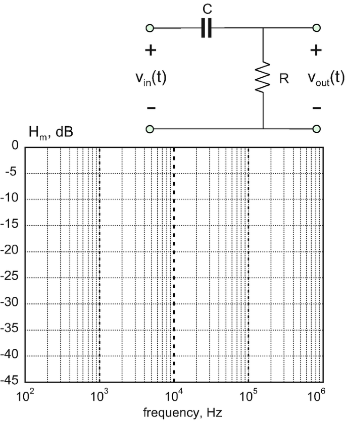
For the filter circuit shown in the following figure, given that $R=100\kern0.5em \mathrm{k}\Omega$ and $C=159\kern0.5em \mathrm{pF}$:

• A. Create the amplitude Bode plot by finding transfer function values for (at least) every decade.

• B. Label the break frequency.

• C. Label the filter passband.

  

Problem 9.20

Repeat the previous problem with $R=100\kern0.5em \mathrm{k}\Omega$ and $C=53\kern0.5em \mathrm{pF}$.

Problem 9.21

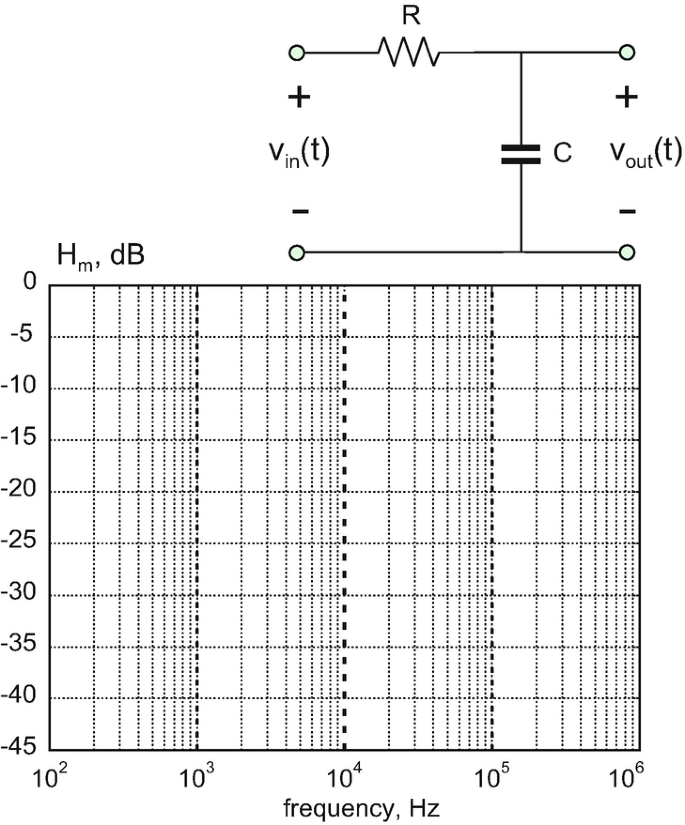
For the filter circuit shown in the following figure, assume the values $R=10\kern0.5em \mathrm{k}\Omega$ and $C=1.59\kern0.5em \mathrm{nF}$.

• A. Create the amplitude Bode plot by finding the transfer function values for (at least) every decade.

• B. Label the break frequency.

• C. Label the filter passband.

  

Problem 9.22

Repeat the previous problem with $R=100\kern0.5em \mathrm{k}\Omega$ and $C=53\kern0.5em \mathrm{pF}$.

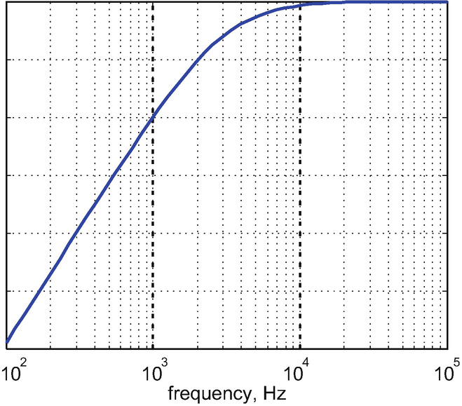
Problem 9.23

An amplitude Bode plot for a certain RC filter is shown in the figure below.

• A. Approximately determine the filter’s resistance R if it is known that $C=265\kern0.5em \mathrm{pF}$. Describe each step of your approach.

• B. Suggest a way to verify your solution.

  

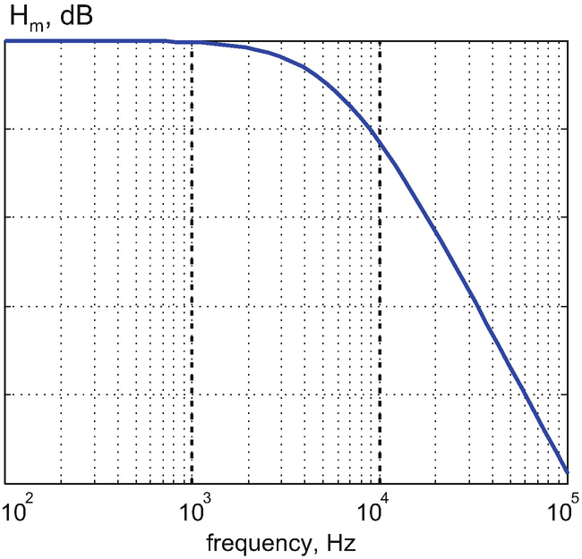
Problem 9.24

An amplitude Bode plot for a certain RC filter is shown in the figure below.

• A. Approximately determine the filter’s capacitance, C, for a given $R=100\kern0.5em \mathrm{k}\Omega$. Describe each step of your approach.

• B. Suggest a way to verify your solution.

  

Problem 9.25

Prove analytically that the amplitude transfer functions of the low-pass filter and the high-pass filter are the mirror reflections of each other about the break frequency in the Bode plot.

9.1.4 Phase Transfer Function and Its Bode Plot

Problem 9.26

Write the phase transfer function for the low-pass RC filter. Repeat for the high-pass RC filter. Show units.

Problem 9.27

The input voltage to a low-pass RC filter has a zero phase. At what frequency in terms of the break frequency f_b is the phase shift at the output equal to −1°, −45°, and −89°?

Problem 9.28

The input voltage to a high-pass RC filter has a zero phase. At what frequency in terms of the break frequency f_b is the phase shift at the output equal to 5°, 45°, and 85°?

Problem 9.29

A low-pass RC filter has the break frequency of 10 kHz. Create the phase Bode plot by finding the transfer function values for (at least) every decade.

Problem 9.30

Repeat the previous problem for a high-pass RC filter with the same break frequency.

9.1.5 Complex Transfer Function: Cascading Filter Circuits

9.1. 6 RL Filter Circuits

Problem 9.31

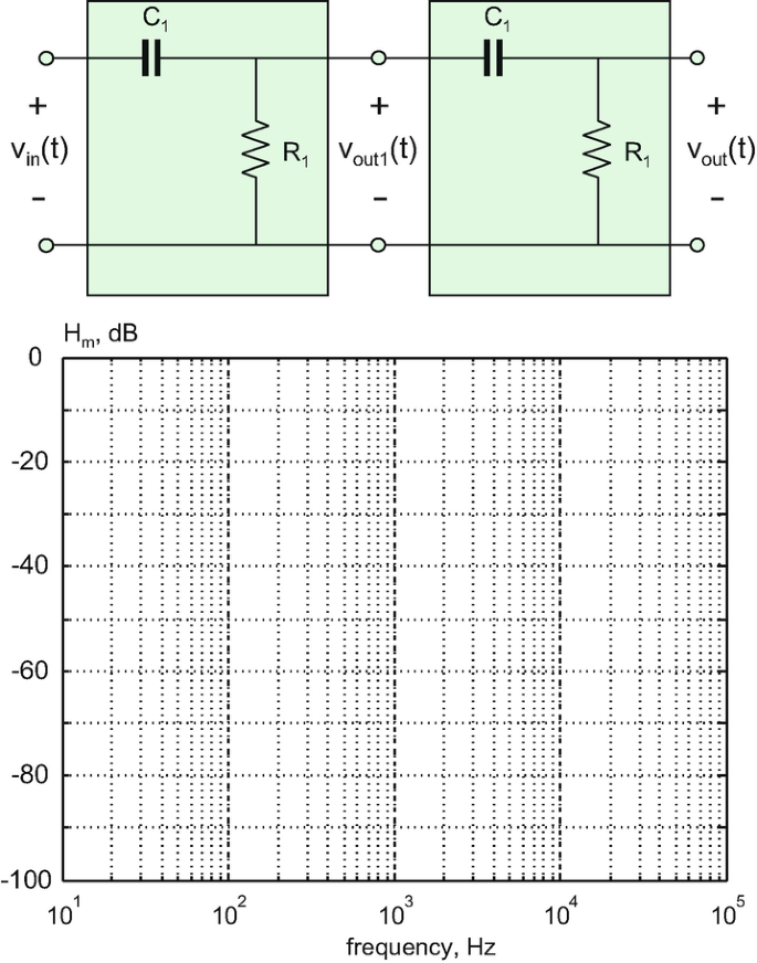
For the filter circuit shown in the figure below, create the amplitude response of the Bode plot by finding transfer function values for (at least) every decade. The two individual filter blocks both have the break frequency of 1 kHz. Assume that the loading effect of the filter stages is negligibly small; in practice, a buffer amplifier stage could be used.

Problem 9.32

• A. Repeat the previous problem for the filter circuit shown in the figure below.

• B. Analytically determine the roll-off per decade in dB.

  

Problem 9.33

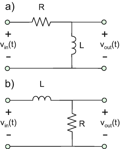
For two RL filter circuits with $R=31.4\kern0.5em \Omega$ and $L=1\kern0.5em \mathrm{mH}$ shown in the figure below:

• A. Determine the break frequency.

• B. Draw the corresponding RC counterpart.

• C. Establish the capacitance values of the RC filters, which assure the equivalent transfer functions, given that the resistances of the RC filters are 100 kΩ in both cases.

  

Problem 9.34

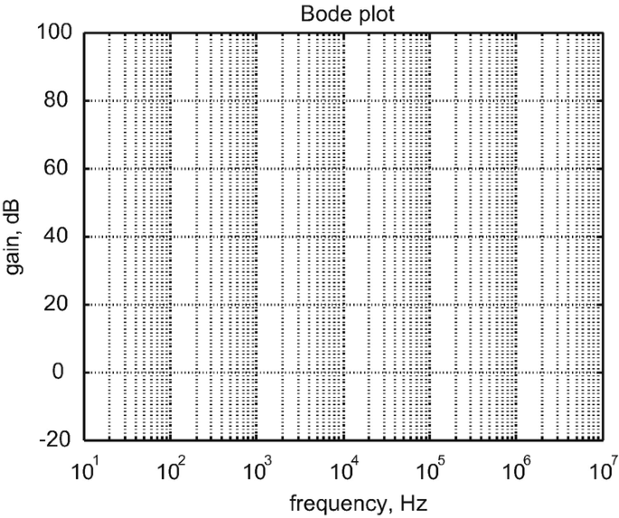
For the filter circuit shown in the figure below, assume the values ${R}_1=628\kern0.5em \Omega$ and ${L}_1=10\kern0.5em \mathrm{mH}$.

• A. Create the amplitude Bode plot by finding transfer function values for (at least) every decade.

• B. Determine the roll-off per decade in dB.

Assume that the loading effect of the filter stages is negligibly small (e.g., a buffer amplifier stage is used).

Problem 9.35

The transfer function of a filter circuit is given by $H\left(\kern0.2em ,f\right)=\frac{1+j\left(\ f/1000\right)}{1+{\left(\ f/1000\right)}^2}$. Create its amplitude and phase Bode plots in the frequency band from 10 Hz to 100 kHz by finding transfer function values for (at least) every decade.

1.2 9.2 Bandwidth of an Operational Amplifier

9.2.1 Bode Plot of the Open- loop Amplifier Gain

9.2.2 Unity-gain Bandwidth Versus Gain-Bandwidth Product

Problem 9.36

An amplifier has the unity-gain bandwidth BW of 5 MHz. What exactly does this mean? Explain and provide equations.

Problem 9.37

Using a manufacturing company’s website (usually it is a more accurate frequently updated source) or the corresponding datasheet, find the unity-gain bandwidth for the following amplifier ICs:

• A. TL082

• B. LM741

• C. LM7171

Problem 9.38

Frequency response of an amplifier is characterized by the open-loop DC gain ${A}_{\mathrm{OL}}(0)=1.41\times {10}^6$ and the break frequency of ${f}_{\mathrm{b}}=20\ \mathrm{Hz}$. Numerically calculate the gain-bandwidth product for the amplifier at:

• A. 20 Hz,

• B. 2 kHz,

• C. 2 MHz.

9.2.3 Model of the Open-Loop AC Gain

Problem 9.39

Frequency response of an amplifier is characterized by the open-loop DC gain ${A}_{\mathrm{OL}}(0)={10}^6$ and the break frequency of ${f}_{\mathrm{b}}=20\ \mathrm{Hz}$. Plot the open-loop gain magnitude in dB over the range of frequencies (the frequency band) from 1 Hz to 10 MHz on the log-log scale (the Bode plot) and label the axes.

Problem 9.40

In the previous problem, find the unity-gain bandwidth BW of the amplifier.

Problem 9.41

Internally compensated LM358-series amplifiers have the unity-gain bandwidth (BW) of 1 MHz. The typical large-signal DC voltage gain at room temperature is 100 V/mV.

• A. Find the open-loop DC gain in dB and the open-loop break frequency f_b.

• B. Find the open-loop gain at 100 Hz, 1 kHz, and 10 kHz.

Problem 9.42

The open-loop gain magnitude of an internally compensated high-frequency amplifier has been given as

$$ {A}_{\mathrm{OL}}\left(100\kern0.5em \mathrm{Hz}\right)=0.9\times {10}^6,\kern1em {A}_{\mathrm{OL}}\left(1\kern0.5em \mathrm{MHz}\right)=1.0\times {10}^2 $$

at room temperature. Determine:

• A. 3-dB break frequency,

• B. DC open-loop gain,

• C. Unity-gain bandwidth BW of the amplifier.

Problem 9.43

Repeat the previous problem for

$$ {A}_{\mathrm{OL}}\left(100\kern0.5em \mathrm{Hz}\right)=0.5\times {10}^6,{A}_{\mathrm{OL}}\left(1\kern0.5em \mathrm{MHz}\right)=1.0\times {10}^2. $$

9.2.4 Model of the Closed-loop AC Gain

9.2.5 Application Example: Finding Bandwidth of an Amplifier Circuit

Problem 9.44

An amplifier with the open-loop gain described by the first-order RC circuit response with ${A}_{\mathrm{OL}}(0)={10}^5$ and ${f}_{\mathrm{b}}=20\kern0.5em \mathrm{Hz}$ is used in a closed-loop inverting configuration with ${R}_2/{R}_1=9$ and ${R}_2/{R}_1=99$, respectively.

• A. Using the template that follows, create the Bode plots for the corresponding frequency response (closed-loop gain), G(f), in the band from 10 Hz to 10 MHz on the same graph. Plot the gain values for (at least) every decade.

• B. Also on the same graph, plot the open-loop gain as a function of frequency.

• C. Determine the bandwidth of the closed-loop amplifier so constructed in every case.

  

Problem 9.45

The unity-gain bandwidth of an amplifier IC is 1 MHz. Determine the bandwidth of the following amplifier circuits:

• A. An inverting amplifier with the gain of −1,

• B. An inverting amplifier with the gain of −10,

• C. A non-inverting amplifier with the gain of 100,

• D. A voltage follower (buffer amplifier).

constructed using the same IC.

9.2.6 Application Example: Selection of an Amplifier IC for Proper Frequency Bandwidth

Problem 9.46

An inverting amplifier with a gain of −20 and a bandwidth of at least 200 kHz is needed. Which amplifier chip is appropriate for this circuit (and which is not)?

• A. LM358

• B. TL082

• C. LM741

• D. LM7171

• E. LM8272

Problem 9.47

A non-inverting amplifier with a gain of 31 and a bandwidth of at least 90 kHz is needed. Which amplifier chip is appropriate for this circuit (and which is not)?

• A. TL082

• B. LM7171

• C. LM8272

1.3 9.3 Introduction to Continuous and Discrete Fourier Transform

9.3.1 Meaning and Definition of Fourier Transform

Problem 9.48

Establish all values of the angular frequency ω in Fig. 9.14b at which the Fourier spectrum F(ω) of a rectangular pulse crosses the frequency axis (becomes zero). Express your result in terms of pulse duration T.

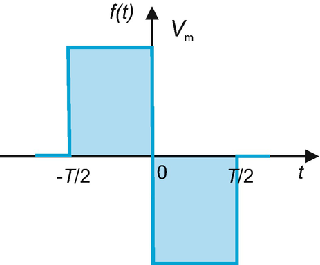
Problem 9.49

• A. Establish the value of the Fourier transform F(ω) for the pulse shown in the following figure at $\omega =0$.

• B. Establish the complete pulse spectrum F(ω) at all values of angular frequency ω.

  

Problem 9.50

Establish the Fourier transform F(ω) for the following voltage signals in time domain:

• A. ${\displaystyle \begin{array}{cc}f(t)=A\sin \left(\frac{\pi }{2}t\right),& -2\le t<2\\ {}\kern-3.4em f(t)=0,& \mathrm{otherwise}\end{array}}$

• B. ${\displaystyle \begin{array}{cc}f(t)=A\cos \left(\frac{\pi }{2}t\right),& -2\le t<2\\ {}\kern-3.4em f(t)=0,& \mathrm{otherwise}\end{array}}$

Problem 9.51

Show that for an arbitrary real voltage signal f(t):

• A. The real part of F(ω) is an even function of angular frequency ω.

• B. The imaginary part of F(ω) is an odd function of angular frequency ω.

• C. The magnitude of F(ω) is an even function of angular frequency ω.

• D. Replacing ω by $-\omega$ generates the complex conjugate of F(ω); in other words, $F\left(-\omega \right)={F}^{\ast}\left(\omega \right)$.

9.3.2 Mathematical Properties of Fourier Transform

Problem 9.52

The Fourier transform of f(t) is F(ω). What is the Fourier transform of ${d}^2f(t)/d{t}^2-2\underset{-\infty }{\overset{t}{\int }}f\left(\tau \right) d\tau$?

Problem 9.53

The Fourier transform of f(t) is F(ω). What is the Fourier transform of $f\left(-t\right)$?

Problem 9.54

The function f(t)cos ω₀t is an amplitude-modulated signal : a high-frequency carrier cos ω₀t, which is transmitted wirelessly, has a low-frequency envelope f(t), which carries information and is being demodulated at the receiver. If the Fourier transform of f(t) is F(ω), what is the Fourier transform of f(t)cos ω₀t?

Problem 9.55

If f(t) represents the voltage across a 1-Ω load, then f²(t) is the power delivered to the load and $\underset{-\infty }{\overset{\infty }{\int }}{f}^2(t) dt$ is the total energy delivered to the load. Prove Parseval’s theorem ,

$$ \underset{-\infty }{\overset{\infty }{\int }}{f}^2(t) dt=\frac{1}{2\pi}\underset{-\infty }{\overset{\infty }{\int }}{\left|F\left(\omega \right)\right|}^2 d\omega, $$

which relates the total energy to an integral of the energy spectral density , ${\left|F\left(\omega \right)\right|}^2=F\left(\omega \right){F}^{\ast}\left(\omega \right)$, of the signal.

Hint: Use the reversal property of the Fourier transform given by Eq. (9.26).

Problem 9.56

Based on Parseval’s theorem established in the previous problem, find the value of the integral $\underset{-\infty }{\overset{\infty }{\int }}{\operatorname{sinc}}^2(t) dt$.

9.3.3 Discrete Fourier Transform and Its Implementation

Problem 9.57

You are using the discrete Fourier transform of length 8 ($N=8$) for a signal $f(t)=\sin t$ over a time interval from 0 to 2π s.

• A. Compute all sampling points in the time domain.

• B. Compute all sampling points in the frequency domain.

• C. Compute equivalent frequency samples using negative frequencies.

• D. Compute all discrete samples f[n].

• E. Compute all discrete samples F[m] using the definition of the discrete Fourier transform. Explain the physical meaning of their values.

• F. Repeat the previous step using function fft of MATLAB. Compare both sets of F[m].

• G. Restore all discrete samples f[n] using the definition of the inverse discrete Fourier transform. Compare them with the exact function values.

• H. Repeat the previous step using function ifft of MATLAB. Compare both sets of f[n].

Problem 9.58

Repeat the previous problem for the signal $f(t)=\cos t$. All other parameters remain the same.

Problem 9.59

For Problem 9.57, establish and prove a discrete version of Parseval’s theorem formulated in Problem 9.55.

Problem 9.60

An input signal to a filter has a discrete frequency spectrum $F\left[m\right],\kern1em m=0,\dots, N-1$ computed via the FFT. You are given filter transfer function H computed at $\frac{N}{2}+1$ frequency points of the FFT, $\mathbf{H}\left[m\right],\kern1em m=0,\dots, N/2$. Compute the discrete spectrum of the filter’s output to be fed into the IFFT.

9.3.6 Application Example: Numerical Differentiation via the FFT

9.3.7 Application Example: Filter Operation for an Input Pulse Signal

Problem 9.61*

Present the text of a MATLAB script that numerically differentiates the input signal $f(t)=\sin t$ over the time interval from 0 to 4π s using the FFT with 4096 sampling points and plot the resulting signal derivative.

Problem 9.62

Repeat the previous problem for the signal $f(t)=\exp \left(-{\left(t-2\pi \right)}^2\right)$. All other parameters remain the same.

Problem 9.63

A monopolar pulse $f(t)=\exp \left(-2{\left(t-5\right)}^2\right),\kern1em 0\kern0.5em \le t<10\kern0.5em \mathrm{s}$ is an input to a series combination of two identical first-order high-pass filters. Find the output of the filter combination when the (angular) break frequency is given by:

• A. ${\omega}_0=0.5\ \mathrm{rad}/\mathrm{s}$

• B. ${\omega}_0=10\ \mathrm{rad}/\mathrm{s}$

Use the FFT and IFFT with $N=64$. Plot the filter output and explain the output signal behavior in every case.

Problem 9.64

A bipolar pulse $f(t)=\left(5-t\right)\exp \left(-2{\left(t-5\right)}^2\right),\kern0.5em 0\le t<10\ \mathrm{s}$ is an input to a first-order low-pass filter. Find the filter output when its (angular) break frequency is given by:

• A. ${\omega}_0=0.5\ \mathrm{rad}/\mathrm{s}$

• B. ${\omega}_0=5\ \mathrm{rad}/\mathrm{s}$

Use the FFT and IFFT with $N=64$. Plot the filter output along with the input signal on the same graph and explain the output signal behavior in both cases.